Interacting Neural Networks

Abstract

Several scenarios of interacting neural networks which are trained either in an identical or in a competitive way are solved analytically. In the case of identical training each perceptron receives the output of its neighbour. The symmetry of the stationary state as well as the sensitivity to the used training algorithm are investigated. Two competitive perceptrons trained on mutually exclusive learning aims and a perceptron which is trained on the opposite of its own output are examined analytically. An ensemble of competitive perceptrons is used as decision-making algorithms in a model of a closed market (El Farol Bar problem or Minority Game); each network is trained on the history of minority decisions. This ensemble of perceptrons relaxes to a stationary state whose performance can be better than random.

Simple models of neural networks describe a wide variety of phenomena in neurobiology and information theory. Neural networks are systems of elements interacting by adaptive couplings which are trained by a set of examples. After training they function as content addressable associative memory, as classifiers or as prediction algorithms. Using methods of statistical physics many of these phenomena have been elucidated analytically for infinitely large neural networks [1, 2].

Most studies of feed-forward neural networks have concentrated on a single network learning a fixed rule, which is usually a second network, the so-called teacher. The teacher network is presenting examples, sets of input/output data, and the student network is adapting its weights to this set of examples. In an on-line training scenario each example is presented only once, hence training is a dynamical process [3, 4]. The teacher network may also generate a time series of output numbers [5, 6], and the student learns by following the time series. The weights of the teacher network are fixed in this scenario.

Many phenomena in biology, social and computer science may be modeled by a system of interacting adaptive algorithms (see e.g. [7]). However, little is known about general properties of such systems. In this paper we derive an analytic solution of a system of interacting neural networks. Each network is a simple perceptron with an $N$-dimensional weight vector. These networks receive an identical input vector, produce output bits and learn from each other. In Section I, each network is trained by the output of its neighbour, with a cyclic flow of information. By iterating the training step for randomly chosen input vectors, the dynamical process relaxes to a stationary state. In the limit of $N\rightarrow\infty$ we describe the process by ordinary differential equations for a few order parameters, similiar to the usual student/teacher scenario [3, 8]. We identify the symmetries of the stationary state and find phase transitions when increasing the learning rate of the training steps.

In Section II and III we study different training scenarios with two interacting perceptrons and various learning algorithms.

In Section IV we apply the system of interacting networks to a problem of game theory called the minority game, which is derived from the El-Farol Bar problem [9, 10]. We consider a set of agents who have to make a binary decision. Each agent wins only if he/she belongs to the minority of all decisions. This process is iterated. Each agent has to develop an algorithm which makes a decision according to the history of the global minority decisions. The problem recently received a lot of attention in the context of statistical physics [11]. Here we follow a novel approach: Each agent uses a perceptron for making his/her decision, and each perceptron is trained on the minority of all output bits.

I Mutual Learning, symmetric case

In this section we investigate a system of interacting neural networks as follows: several identical networks are arranged on an oriented ring. All networks receive an identical input and produce different output according to their weight vectors. Each network is trained by the output of its neighbour on the ring. This process is iterated until a stationary state is reached in which the norms and angles between the weight vectors no longer change. We are interested in the properties of this stationary state.

We consider the simplest feed-forward networks, an ensemble of $K$ simple perceptrons, which are represented by $N$-dimensional weight vectors ${\mathbf{w}}_{i}$ $(i=1,\dots,K)$ and which map a common input vector ${\mathbf{x}}$ onto binary outputs $\sigma_{i}=\mbox{sign}({\mathbf{x}}\!\cdot\!{\mathbf{w}}_{i})$. As order parameters we use the norms $w_{i}=|{\mathbf{w}}_{i}|$ and the respective overlaps $R_{ij}={\mathbf{w}}_{i}\!\cdot\!{\mathbf{w}}_{j}$ or $\cos(\theta_{ij})={\mathbf{w}}_{i}\!\cdot\!{\mathbf{w}}_{j}/w_{i}w_{j}$. When only two perceptrons are considered, the subscript is dropped: $\cos(\theta)={\mathbf{w}}_{1}\!\cdot\!{\mathbf{w}}_{2}/w_{1}w_{2}$. The components of the input vector (or pattern) are Gaussian with mean 0 and variance 1, yielding ${\mathbf{x}}\!\cdot\!{\mathbf{x}}=O(N)$.

The updates are of the form

$${\mathbf{w}}_{i}^{+}={\mathbf{w}}_{i}+(\eta_{i}/N)f(\sigma_{i},s)s\,{\mathbf{x}}$$ (1)

for unnormalized weights or

$${\mathbf{w}}_{i}^{+}=\frac{{\mathbf{w}}_{i}+(\eta_{i}/N)f(\sigma_{i},s)s\,{\mathbf{x}}}{|{\mathbf{w}}_{i}+(\eta_{i}/N)f(\sigma_{i},s)s\,{\mathbf{x}}|}$$ (2)

for normalized ${\mathbf{w}}_{i}$. The $+$ denotes a quantity after one learning step, $\eta_{i}$ is the learning rate, $s$ is the desired output, and $f(\sigma_{i},s)$, the so-called weight function, defines the learning algorithm. We mostly use $f=1$ (the Hebbian rule, called $H$ from now on) and $f=\Theta(-\sigma_{i}s)$ (the perceptron learning rule, abbreviated $P$ [1]), and the respective variations where the ${\mathbf{w}}_{i}$ are kept normalized, denoted as $HN$ and $PN$ respectively.

We derive differential equations for the order parameters in the thermodynamic limit $N\rightarrow\infty$ by taking the scalar product of the update rules and introducing a time variable $\alpha=p/N$, where $p$ is the number of patterns shown so far. We use the analytic tools which were previously developed for the teacher/student scenario [4, 3]. If the order parameters are self-averaging (see [12] for criteria of self-averaging in this context), integrating over the distribution of patterns gives deterministic differential equations for the order parameters as $N\rightarrow\infty$. The required averages are listed in the appendix.

A Perceptron learning rule

We first restrict ourselves to two perceptrons that try to come to an agreement by learning the output of the respective other perceptron.

For rule $P$ with identical learning rates $\eta_{1}=\eta_{2}=\eta$, the update rule is

$${\mathbf{w}}_{1}^{+} = {\mathbf{w}}_{1}+\frac{\eta}{N}{\mathbf{x}}\,\sigma_{2}\Theta(-\sigma_{1}\,\sigma_{2});$$ (3)

$${\mathbf{w}}_{2}^{+} = {\mathbf{w}}_{2}+\frac{\eta}{N}{\mathbf{x}}\,\sigma_{1}\Theta(-\sigma_{1}\,\sigma_{2}).$$ (4)

The sum of both vectors is conserved under this rule: if a learning step takes place, it has the same direction and absolute value, but different signs for the two vectors. This conservation can be used to link $w_{1}$ and $w_{2}$ to $\cos(\theta)$: assuming that $w_{1}=w_{2}=w$ and starting from $\theta_{0}=\pi/2$, simple geometry gives $w_{0}/\sqrt{2}=\cos(\theta/2)w$. The conservation is also visible in the differential equations that can be derived using the described formalism:

$$\frac{dw_{1}}{d\alpha} = -\frac{\eta}{\sqrt{2\pi}}(1-\cos(\theta))+\frac{\eta^{2}\theta}{2w_{1}\pi};$$ (5)

$$\frac{dw_{2}}{d\alpha} = -\frac{\eta}{\sqrt{2\pi}}(1-\cos(\theta))+\frac{\eta^{2}\theta}{2w_{2}\pi};$$ (6)

$$\frac{dR}{d\alpha} = \frac{\eta}{\sqrt{2\pi}}(1-\cos(\theta))(w_{1}+w_{2})-\eta^{2}\frac{\theta}{\pi}.$$ (7)

If the right-hand side of 5 and 6 vanish, so does 7. There is a curve of fixed points of the system given by the equation

$$w=\frac{\eta}{\sqrt{2\pi}}\frac{\theta}{1-\cos(\theta)}.$$ (8)

Using the relation $w=w_{0}/(\sqrt{2}\cos(\theta/2))$, this can be solved numerically to give the fixed point of $\cos(\theta)$ as a function of the scaled learning rate $\eta/w_{0}$, as shown in Fig. 1. For small learning rates, the perceptrons come to good agreement, while large $\eta$ leads to antiparallel vectors.

Geometrically, this can be understood as follows: each learning step has a component parallel to the plane spanned by ${\mathbf{w}}_{1}$ and ${\mathbf{w}}_{2}$, which decreases the distance between the vectors, and a perpendicular component, which increases the distance (see Fig. 2). Equilibrium is reached when a typical learning step no longer changes the angle, i.e. the vectors stay on a cone around ${\mathbf{w}}_{1}+{\mathbf{w}}_{2}$. The radius of this cone increases with growing $\eta$.

B Perceptron learning with normalized weights

A similar calculation can be done for the perceptron learning rule with normalized weights ($PN$), where the length $w_{i}$ of the weight vectors is set to $1$ after each step. The perceptrons move on a hypersphere of radius 1; in equilibrium, the average learning step leads back onto that sphere before the vectors are normalized again.

We derive the following differential equation for $R=\cos(\theta)$:

$$\frac{dR}{d\alpha}=(R+1)\left(\sqrt{\frac{2}{\pi}}\eta(1-R)-\eta^{2}\frac{\theta}{\pi}\right).$$ (9)

Fixed points are $R=1$, $R=-1$ and

$$\frac{\eta}{\sqrt{2\pi}}\frac{\theta}{1-\cos(\theta)}=1.$$ (10)

It is not a coincidence that this is equivalent to (8) if $w$ is set to 1. The fixed point of (10) at $R=1$ is repulsive; the one at $R=-1$ is unstable for $\eta<4/\sqrt{2\pi}\doteq 1.60$. A solution of (10) can only be found for $\eta\leq\eta_{c}\doteq 1.816$, which corresponds to $\cos(\theta)\doteq-0.689$.

Simulations show that the system relaxes to the fixed point given by Eq. (10) for $\eta<\eta_{c}$ and jumps to $R=-1$ for larger $\eta$ (see Fig. 3). This behaviour shows the characteristics of a first-order phase transition.

Hence for small learning rates the two perceptrons relax to a state of nearly complete agreement, $\theta\approx 0$. Increasing $\eta$ leads to a nonzero angle between the two vectors up to $\theta\approx 133^{\circ}$. At this rate the system jumps to complete disagreement, $\theta=180^{\circ}$.

C Mutual learning on a ring

The mutual learning-scenario can be generalized to $K$ perceptrons: perceptron $i$ learns from perceptron $i+1$ if they disagree, with cyclic boundary conditions. Under rule $P$, the total sum of vectors is conserved again: as many perceptrons take a step in one direction as in the opposite.

Performing the necessary averages for the equations of motion would involve Gaussian integrals over $K-1$ correlated variables with $\Theta$-functions – it is not clear to us whether this can be done analytically in general cases. However, we find in simulations that the fixed point for rule $P$ is completely symmetric: there is only one angle $\theta$ between all pairs of perceptrons. Assuming that relation (8) still holds, and using the conservation of $\sum{\mathbf{w}}_{i}$, one can derive

$$\frac{\eta}{\sqrt{2\pi}}\frac{\theta}{1-\cos(\theta)}=\frac{w_{0}}{\sqrt{1+(K-1)\cos(\theta)}}.$$ (11)

The largest angle that the perceptrons can take is $\cos(\theta)=-1/(K-1)$, corresponding to a $K$-cornered hypertetrahedron. This happens when $|\sum{\mathbf{w}}_{i}|$ is negligible w.r.t $w_{i}$. Simulations confirm that (11) holds, as can be seen in Fig. 1

Similar to the case of two networks, all perceptrons agree with each other for small learning rate $\eta\rightarrow 0$. For larger rates the system relaxes to a state of high symmetry where all mutual angles between the $K$ weight vectors are identical, $\theta_{ij}=\theta$. Note that the symmetry is higher than the topology of the flow of information (the ring). For high rates $\eta\rightarrow\infty$ the system relaxes to a state of maximal disagreement, i.e. the largest possible mutual angle $\theta$ that is still compatible with a symmetric arrangement.

For rule $PN$, the sum of the weights is not preserved. The fixed point of the dynamics follows the curve for two normalized weights described by Eq. (10) in a completely symmetric configuration. When the hypertetrahedron angle is reached and $\sum{\mathbf{w}}_{i}$ vanishes, the symmetry is partly broken. There are now different angles to nearest neighbours, next-nearest neighbours etc., so the angles split up into $(K-1)/2$ different branches for odd $K$ and $K/2-1$ for even $K$. Note that the system still has the symmetry of the ring.

With odd $K$, increasing $\eta$ increases the angle between nearest neighbours, up to some limit value. This angle is not the maximum nearest-neighbour angle allowed for by the geometric constraints, but seems to decrease with increasing K.

In the case of even $K$, simulations show a second transition at some higher value of $\eta$, where the vectors split into two antiparallel clusters, thus maximizing the nearest-neighbour angle. The learning rate at which this transition typically appears during the run of the program increases with $N$. The conclusion is that the antiparallel fixed point is not stable in the $N\rightarrow\infty$ limit, but de facto stable in simulations because the self-averaging property of the ODEs breaks down at this point.

One may ask which symmetries survive if the perceptrons are allowed to have different individual learning rates. A close look reveals that for rule $P$, there is a more general conserved quantity: $\sum_{i}^{K}{\mathbf{w}}_{i}/\eta_{i}$. Simulations show that the angles $\theta_{ij}$ again relax to a completely symmetric configuration depending on the average $\eta$ and the initial value of the new conserved quantity, while the norms $w_{i}$ are proportional to the respective learning rates $\eta_{i}$. For rule $PN$, variations in the learning rates not only lead to slightly different curves for each of the angles with individually different $\eta_{c}$, they also suppress the transition to the antiparallel state that is observed for even $K$.

D Hebbian learning

The reason why $P$ and $PN$ lead to antiparallel orientation of the weight vectors for larger learning rates is that they concentrate on cases where the networks disagree. Algorithms that reinforce what both networks agree on are more successful, as can be seen for rule $H$ for two perceptrons.

The differential equations are

$$\frac{dw_{i}}{d\alpha} = \eta\sqrt{\frac{2}{\pi}}\cos(\theta)+\frac{\eta^{2}}{2w_{i}};$$ (12)

$$\frac{dR}{d\alpha} = \eta\sqrt{\frac{2}{\pi}}(w_{1}+w_{2})+\eta^{2}(1-\frac{2\theta}{\pi}).$$ (13)

This system has no common fixed point, which means that the $w_{i}$ grow without bounds. The asymptotic behaviour can be seen from the equation for $\cos(\theta)$. Assuming that $w_{1}=w_{2}=w$, we find

$$\frac{d\cos(\theta)}{d\alpha}=\frac{\eta}{w}\frac{4}{\sqrt{2\pi}}(1-\cos(\theta)^{2})+\frac{\eta^{2}}{w^{2}}\left(1-\cos(\theta)-\frac{2\theta}{\pi}\right).$$ (14)

By taking $w\approx\sqrt{2/\pi}\eta\alpha$, the ODE leads to $1-\cos(\theta)\propto\alpha^{-4}$ for $\alpha\rightarrow\infty$. This means that $\theta\propto\alpha^{-2}$.

Simulations agree with the numerical integration of Eqs. (13), with the exception of very large $\alpha$ and correspondingly small $\theta$ (see Fig. 4). This is not surprising, since the $\alpha^{-2}$-decay is an effect of patterns that are classified differently. As long as the perceptrons give the same output on all patterns, $w_{1}$ and $w_{2}$ grow linearly, but the difference ${\mathbf{w}}_{1}-{\mathbf{w}}_{2}$ does not change, leading to $\theta\propto\alpha^{-1}$. This is observed in simulations for small angles, where no patterns happened to be classified differently on the considered timescale. Mathematically, this is related to a breakdown of the self-averaging properties of Eqs. (13) at the point $\theta=0$.

II Mutual learning, competition

In the previous section, all of the neural networks behave in the same way. Each perceptron tries to learn the output of its neighbour, and only the initial weight vectors are chosen randomly and differ from each other. Now we investigate a scenario where two networks behave differently. Network 1 is trying to simulate network 2 while 2 ist trained on the opposite of the opinion of 1. This scenario describes a competition between two adaptive algorithms. If 2 is completely successful, the overlap is $\cos(\theta)=-1$, and perceptron 1 always fails in its prediction, and vice versa. A motivation from game theory can be drawn from the game of penny matching, where both players make a binary decision simultaneously. One player wins if the decisions are the same, the other if they are different.

A Rule $P$

If both perceptrons use rule $P$ for their respective learning aim, the update rules are

$${\mathbf{w}}_{1}^{+} = {\mathbf{w}}_{1}+(\eta_{1}/N){\mathbf{x}}\sigma_{2}\Theta(-\sigma_{1}\sigma_{2});$$ (15)

$${\mathbf{w}}_{2}^{+} = {\mathbf{w}}_{2}-(\eta_{2}/N){\mathbf{x}}\sigma_{1}\Theta(\sigma_{1}\sigma_{2}).$$ (16)

The corresponding differential equations for the order parameters are

$$\frac{dw_{1}}{d\alpha} = -\frac{\eta_{1}}{\sqrt{2\pi}}(1-\cos(\theta))+\frac{\eta_{1}^{2}}{2w_{1}}\frac{\theta}{\pi}$$ (17)

$$\frac{dw_{2}}{d\alpha} = -\frac{\eta_{2}}{\sqrt{2\pi}}(1+\cos(\theta))+\frac{\eta_{2}^{2}}{2w_{2}}(1-\frac{\theta}{\pi});$$ (18)

$$\frac{dR}{d\alpha} = \frac{\eta_{1}w_{2}}{\sqrt{2\pi}}(1-\cos(\theta))-\frac{\eta_{2}w_{1}}{\sqrt{2\pi}}(1+\cos(\theta)).$$ (19)

The common fixed point for these equations is $w_{i}=\sqrt{2\pi}\eta_{i}/4$, $\cos(\theta)=0$. This is hardly surprising, since none of the perceptrons has a better algorithm than the other. The learning rate only rescales the weight vectors; the ratio $\eta_{i}/w_{i}$, which determines how fast the direction of ${\mathbf{w}}_{i}$ in weight space can change, is independent of $\eta$ at the fixed point.

B Rule $H$

The picture is slightly different if both perceptrons learn from every pattern they see. The resulting differential equations are

$$\frac{dw_{1}}{d\alpha} = \sqrt{\frac{2}{\pi}}\eta_{1}\cos(\theta)+\frac{\eta_{1}^{2}}{2w_{1}};$$ (20)

$$\frac{dw_{2}}{d\alpha} = -\sqrt{\frac{2}{\pi}}\eta_{2}\cos(\theta)+\frac{\eta_{2}^{2}}{2w_{2}};$$ (21)

$$\frac{dR}{d\alpha} = \sqrt{\frac{2}{\pi}}\eta_{1}w_{2}-\sqrt{\frac{2}{\pi}}\eta_{2}w_{1}-\eta_{1}\eta_{2}(\pi-2\theta).$$ (22)

The fixed point of $R$ is reached if $\theta=\pi/2$ and $\eta_{1}/w_{1}=\eta_{2}/w_{2}$, i.e. the vectors are perpendicular and the scaled learning rates $\eta_{i}/w_{i}$ are the same for both perceptrons. Under these conditions, the equations for $w_{i}$ can be solved: $w_{i}=\eta_{i}(\alpha+(w_{i,0}/\eta_{1})^{2})^{1/2}$, so $w_{i}$ shows the $\sqrt{\alpha}$-scaling typical for random walks. Geometrically, the Hebb rule adds corrections to the weight vector that are on average parallel to the teacher vector. Since the teacher is moving at the same angular velocity as the student, the movement of both vectors resembles a random walk. Again, $\eta$ only sets the temporal and spatial scale.

C Rule $P$ vs. rule $H$

The result of the competition becomes more interesting when both perceptrons use different algorithms. For example, we let perceptron 1 use rule $P$, while 2 uses $H$. The derivation of the differential equations is again straightforward:

$$\frac{dw_{1}}{d\alpha} = -\frac{\eta_{1}}{\sqrt{2\pi}}(1-\cos(\theta))+\frac{\eta_{1}^{2}}{2w_{1}}\frac{\theta}{\pi};$$ (23)

$$\frac{dw_{2}}{d\alpha} = -\sqrt{\frac{2}{\pi}}\eta_{2}\cos(\theta)+\frac{\eta_{2}^{2}}{2w_{2}};$$ (24)

$$\frac{dR}{d\alpha} = -\sqrt{\frac{2}{\pi}}\eta_{2}w_{1}+\frac{\eta_{1}w_{2}}{\sqrt{2\pi}}(1-\cos(\theta))+\frac{\eta_{1}\eta_{2}\theta}{\pi}.$$ (25)

They have a common fixed point defined by

$$\theta\frac{\cos(\theta)^{2}}{(1-\cos(\theta))^{2}} = \frac{\pi}{4};$$ (26)

$$w_{1} = \frac{\eta_{1}}{\sqrt{2\pi}}\frac{\theta}{1-\cos(\theta);}$$ (27)

$$w_{2} = \frac{\sqrt{2\pi}}{4}\frac{\eta_{2}}{\cos(\theta)}.$$ (28)

These equations can be solved numerically and yield $\cos(\theta)\doteq 0.459$, $w_{1}\doteq 0.806\eta_{1}$ and $w_{2}\doteq 1.37\eta_{2}$. Although perceptron 1 makes less use of the provided information, it wins the competition: the perceptron using rule $H$ has a smaller $\eta/w$-ratio and is thus less flexible.

D Normalized weights

By setting the weights to 1 after each learning step, a new length scale is introduced, leading to a more complex dependence of the solution on the learning rates. For brevity, we only give the differential equations for the different learning rules and explain some common features. If both networks use rule $PN$, the ODE is

$$\frac{dR}{d\alpha}=\frac{1}{\sqrt{2\pi}}(\eta_{1}(1-R)-\eta_{2}(1+R))+\frac{R}{\sqrt{2\pi}}(\eta_{1}(1-R)+\eta_{2}(1+R))-\frac{R}{2\pi}(\eta_{1}^{2}\theta+\eta_{2}^{2}(\pi-\theta));$$ (29)

for rule $HN$ we find

$$\frac{dR}{d\alpha}=\sqrt{\frac{2}{\pi}}(\eta_{2}-\eta_{1})(R^{2}-1)-\frac{R}{2}(\eta_{1}^{2}+\eta_{2}^{2})-\eta_{1}\eta_{2}(1-\frac{2\theta}{\pi});$$ (30)

and if rule $PN$ is used by perceptron 1 and $HN$ by 2, the equation is

$$\frac{dR}{d\alpha} = R\left(\sqrt{\frac{2}{\pi}}\eta_{2}R-\frac{\eta_{2}^{2}}{2}+\frac{\eta_{1}}{\sqrt{2\pi}}(1-R)-\frac{\eta_{1}^{2}}{2}\frac{\theta}{\pi}\right)$$ (32)

$$+\frac{\eta_{1}}{\sqrt{2\pi}}(1-R)-\sqrt{\frac{2}{\pi}}\eta_{2}+\eta_{1}\eta_{2}\frac{\theta}{\pi}.$$

The behaviour of the fixed point is similar in all cases (see Fig. 5):

• if, say, $\eta_{2}$ is fixed and $\eta_{1}\rightarrow 0$, $R$ goes to a value $R\neq-1$. This is expected, since both $PN$ and $HN$ only achieve finite values of $R$ for fixed teachers.

• if both perceptrons use the same algorithm with the same learning rate, the result is $R=0$, as expected.

• if $\eta_{i}\rightarrow\infty$ for either $i$, $R\rightarrow 0$. Infinite learning rate means that in every time step the perceptron discards all the information it previously had, replacing it with the current $\pm{\mathbf{x}}$. Theoretically, that makes it predictable for the other network; in practice, both agents are confused. The notable exception is the case of $PN$ vs. $HN$, where a non-vanishing $R$ results if both $\eta_{i}\rightarrow\infty$ with a finite ratio $\eta_{1}/\eta_{2}$.

III Confused Teacher

For any prediction algorithm there is a bit sequence for which this algorithm fails completely, with $100\%$ error [13]. In fact, such a sequence is easily constructed: Just take the opposite of the predicted bit at each time step. In Ref. [13] a perceptron was used for the prediction algorithm.

Here we do not consider bit sequences. However, it turns out that many statistical properties of the prediction algorithm are similar when random inputs are used instead of a window of the antipredictable bit sequence. Hence we consider the following scenario: Preceptron 1 is trained on the negative of its own output. Perceptron 2 is trained on the output of perceptron 1.

This is similar to the teacher/student model where the teacher weight vector performs a random walk [8]. But here the teacher is “confused”, it does not believe its own opinion and learns the opposite of it.

The update rule of perceptron 1 now only depends on its own output:

$${\mathbf{w}}_{1}^{+}={\mathbf{w}}_{1}-(\eta/N){\mathbf{x}}\sigma_{1}.$$ (33)

Geometrically speaking, the vector performs a directed random walk in which every learning step has a negative overlap with the current vector. An equilibrium length is reached when a typical learning step leads back onto the surface of an $N$-dimensional hypersphere. This fixed point of $w_{1}$ is easily calculated to be

$$w_{1}=\sqrt{2\pi}\eta/4\doteq 0.6267\eta,$$ (34)

and the weight vector typically moves on the surface of a hypersphere of that radius.

A Rule $H$

What happens if a second perceptron tries to follow the output of the confused teacher? Again, the results depend entirely on the used algorithm. The simplest case, the Hebb rule, also has a geometrical interpretation that is revealed by a look at the update rule:

$${\mathbf{w}}_{1}^{+} = {\mathbf{w}}_{1}-(\eta/N){\mathbf{x}}\sigma_{1};$$ (35)

$${\mathbf{w}}_{2}^{+} = {\mathbf{w}}_{2}+(\eta/N){\mathbf{x}}\sigma_{1}.$$ (36)

As in section I A, the sum of both vectors is constant, so there is a class of solutions to the ODEs

$$\frac{dw_{1}}{d\alpha} = -\sqrt{\frac{2}{\pi}}\eta+\frac{\eta^{2}}{2w_{1}};$$ (37)

$$\frac{dw_{2}}{d\alpha} = \sqrt{\frac{2}{\pi}}\eta\cos(\theta)+\frac{\eta^{2}}{2w_{2}};$$ (38)

$$\frac{dR}{d\alpha} = \sqrt{\frac{2}{\pi}}\eta(w_{1}-w_{2}\cos(\theta))+\eta^{2}$$ (39)

defined by $w_{1,f}=\sqrt{2\pi}\eta/4$ and $w_{2,f}=-\sqrt{2\pi}\eta/(4\cos(\theta))$. The solution is given by the initial condition, i.e. the initial sum $|{\mathbf{w}}_{1}+{\mathbf{w}}_{2}|$. The fixed point angle can be calculated by applying the cosine theorem to a triangle with side lengths $w_{1,f}$, $w_{2,f}$ and $|{\mathbf{w}}_{1}+{\mathbf{w}}_{2}|$; starting from perpendicular vectors of norm $w_{0}$, one finds

$$\cos(\theta)=-\left(1+\frac{16}{\pi}\left(\frac{w_{0}}{\eta}\right)^{2}\right)^{-1/2}.$$ (40)

Geometrically, for large learning rate $\eta$ both norms become much larger than $w_{0}$; the only way to achieve this while keeping the sum constant is a large angle. For small $\eta$, $w_{1}$ becomes very small compared to the sum, and thus to $w_{2}$. So the direction of ${\mathbf{w}}_{2}$ stays nearly unchanged while ${\mathbf{w}}_{1}$ performs its random walk, leading to nearly perpendicular vectors on average.

B Rule $P$

If perceptron 2 uses rule $P$, the sum of the vectors is not conserved, and a simple geometrical interpretation is not possible. However, the equations of motion can still be solved:

$$\frac{dw_{1}}{d\alpha} = -\sqrt{\frac{2}{\pi}}\eta+\frac{\eta^{2}}{2w_{1}};$$ (41)

$$\frac{dw_{2}}{d\alpha} = -\frac{\eta}{\sqrt{2\pi}}(1-\cos(\theta))+\frac{\eta^{2}}{2w_{2}}\frac{\theta}{\pi};$$ (42)

$$\frac{dR}{d\alpha} = \sqrt{\frac{2}{\pi}}\eta\cos(\theta)-\frac{w_{1}\eta}{\sqrt{2\pi}}(1-c)-\eta^{2}\frac{\theta}{\pi}.$$ (43)

The fixed point of $\cos(\theta)$ is given by the solution of $4\theta/\pi=(1+\cos(\theta))^{2}$, independent from $\eta$. The numerical solution is $\theta\doteq 0.777\pi$, $\cos(\theta)=-0.761$, $w_{2}=0.552\eta$ (in accordance with Ref. [13], where a special case of this problem was solved). Remarkably, the generalization error is larger than 50% - even the “smarter” perceptron learning rule predicts the behaviour of the confused teacher with less success than random guessing would.

C Optimal learning rule

This raises an interesting question: is there any “reasonable” algorithm for perceptrons that allows them to track the confused teacher? If there are algorithms that achieve a positive overlap, one of them has to be the rule that optimizes student-teacher overlap in each time step – the optimal weight function derived by Kinouchi and Caticha [14]:

$$f_{\mbox{opt}}=\frac{w_{2}\tan(\theta)}{\sqrt{2\pi}}\exp\left[-\frac{({\mathbf{x}}\!\cdot\!{\mathbf{w}}_{2})^{2}}{2\tan(\theta)^{2}\;w_{2}^{2}}\right]\frac{1}{\Phi(\sigma_{1}{\mathbf{x}}\!\cdot\!{\mathbf{w}}_{2}/(w_{2}\tan(\theta)))},$$ (44)

where $\Phi(x)=\int_{-\infty}^{x}\exp(-z^{2}/2)/\sqrt{2\pi}dz$. If $w_{1}$ is set to its fixed point for simplicity’s sake, calculation yields the following ODEs for $\cos(\theta)$ and $w_{2}$:

$$\frac{d\cos(\theta)}{d\alpha} = \frac{1}{4\pi}\frac{\sin(\theta)^{2}}{\cos(\theta)}\,I-\frac{2}{\sqrt{2\pi}w_{1}\cos(\theta)};$$ (45)

$$\frac{dw_{2}}{d\alpha} = \frac{w_{2}}{4\pi}\tan(\theta)^{2}\,I,\mbox{\ \ \ where}$$ (46)

$$I = \int_{-\infty}^{\infty}\frac{1}{\sqrt{2\pi}}\exp\left(-\frac{1+\cos(\theta)^{2}}{2\sin(\theta)^{2}}x^{2}\right)\frac{1}{\Phi(-x\cot(\theta))\Phi(x\cot(\theta))}dx.$$ (47)

Calculating whether $\cos(\theta)=0$ is in fact a fixed point of the confused teacher/optimal student scenario is problematic, since the optimal weight function (44) diverges at $\theta=\pi/2$. However, the numerical solution of Eqs. (45) and (46) shows clearly that even starting from $\cos(\theta)=1$, the system evolves towards $\theta=\pi/2$, which indeed seems to be the upper limit for success. Simulations of the learning process again agree weel with our theory (see Fig. 6).

D Rule $HN$

There is a way of achieving a positive overlap with the confused teacher with simple learning rules: if the teacher perceptron is “slowed down” by keeping its weights normalized and setting $\eta$ to some small value, a student using $PN$ or $HN$ can track the teacher nearly perfectly for very small learning rates. For simplicity’s sake, let us consider $HN$ with identical learning rates. The differential equation for $R$ is

$$\frac{dR}{d\alpha}=(R+1)\left(\sqrt{\frac{2}{\pi}}(1-R)\eta-\eta^{2}\right),$$ (48)

the fixed points are $R=-1$ or $R=-\sqrt{2/\pi}\eta+1$. This result is again confirmed by simulations, as seen in Fig. 7. The fixed point goes to $1$ as $\eta\rightarrow 0$.

IV Perceptrons in the Minority Problem

The concept of interacting neural networks can be applied to a problem that has received much attention recently: the El Farol Bar Problem [9]. The problem was originally inspired by a popular bar that has a limited capacity: if too many people attend, it becomes crowded, and patrons don’t enjoy the evening. In a more special formulation, each agent out of a population of $K$ decides in each time step (each Saturday evening) to take one of two alternatives (go to the bar or stay at home). Those agents who are in the minority win, the others lose. Decisions are made independently; the only information available to agents is the decision of the minority was in the last $N$ time steps.

Many papers (see e.g. [11]) investigated a specific realisation of the model called the Minority Game. In this model each agent has a small number of randomly chosen decision tables (Boolean functions) that prescribe an action based on the previous history, and which of the tables is used is decided according to how successful each one was in the course of the game. It turned out that the success of the game depends on the ratio between the number of players and the size of the history window, and general conclusions on the behaviour of crowded markets were drawn [15, 16].

We will discuss a different approach that yields different behaviour: Each agent $i$ is represented by a perceptron ${\mathbf{w}}_{i}$ that uses the time series ${\mathbf{S}}_{t}=(S_{t},S_{t-1},\ldots,S_{t-N+1})$ of past minority decisions to make a prediction on the next time step. It then learns the output of the minority according to some learning rule.

In our approach, all of the agents are flexible in their decisions. Each agent uses an identical adaptive algorithm which is trained by the history of the game, the only information available to each of the agents. However, each agent uses a different randomly chosen initial state of its network. If all weight vectors of the networks would collapse, all agents would make the same decision, and all would lose. If all weights remained in the random initial state, each agent would make a random guess which yields a reasonable performance of the system. Our calculation shows that training can improve the performance of the system compared to the random state.

Following Ref. [17], we replace the history ${\mathbf{S}}_{t}$ by a random vector ${\mathbf{x}}$. Simulations show that this changes the results only quantitatively, if at all.

This strategy fulfills the restrictions that the original problem posed: the agents do not communicate except through majority decisions, and individual decisions are based on experience (induction or learning) rather than perfect knowledge of the system (deduction). However, since each player uses only one strategy whose parameters can be fine-tuned to the current environment rather than a set of completely different strategies, no quenched bias in the players’ behaviour is to be expected.

A General notes on performance

The commonly used measure of collaboration in the minority problem is the average standard deviation of the sum of outputs of all agents:

$$\frac{\sigma^{2}}{K}=\frac{1}{K}\langle(\sum_{i=1}^{K}\sigma_{i})^{2}\rangle.$$ (49)

If each agent makes random decisions, one gets $\sigma^{2}/K=1$. The probability of two perceptrons $i$ and $j$ giving the same output on a random pattern is $1-\theta_{ij}/\pi$. Any ensemble of vectors ${\mathbf{w}}_{i}$ can be thought of as centered around a center of mass ${\mathbf{C}}=\sum_{i=1}^{K}{\mathbf{w}}_{i}/K$ with a norm $C$ (for random vectors of length 1, $C$ would be of order $\sqrt{K}$). The weights can then be written as ${\mathbf{w}}_{i}={\mathbf{g}}_{i}+{\mathbf{C}}$, with $\sum_{i=1}^{K}{\mathbf{g}}_{i}={\mathbf{0}}$. For the sake of simplicity, we will assume a symmetrical configuration with $g_{i}=1$ and ${\mathbf{g}}_{i}\!\cdot\!{\mathbf{g}}_{j}=-1/(K-1)$ for $i\neq j$. (An ensemble of randomly chosen vectors of norm 1 would give $g_{i}^{2}=1-1/K\pm O(1/\sqrt{N})$ and ${\mathbf{g}}_{i}\!\cdot\!{\mathbf{g}}_{j}=-1/K\pm O(1/\sqrt{N})$.)

The average overlap between different weights is now $R=C^{2}-1/(K-1)$, their average norm $w_{i}=\sqrt{{\mathbf{C}}^{2}+1}$. With this, Eq. (49) can be evaluated:

$$\frac{\sigma^{2}}{K} = \frac{1}{K}\left\langle\sum_{i=1}^{K}1+\sum_{i=1}^{K}\sum_{j\neq i}^{K}\mbox{sign}({\mathbf{x}}\!\cdot\!{\mathbf{w}}_{i})\mbox{sign}({\mathbf{x}}\!\cdot\!{\mathbf{w}}_{j})\right\rangle_{{\mathbf{x}}}$$ (50)

$$= 1+(K-1)\left(1-\frac{2}{\pi}\arccos\left(\frac{C^{2}-1/(K-1)}{C^{2}+1}\right)\right).$$ (51)

If $C$ is set to 0 and $K$ is large, a linear expansion of the arccos term in Eq. (51) gives $\sigma^{2}_{opt}/K\approx 1-2/\pi\doteq 0.363$. The small anticorrelations (of order $1/K$) between the vectors suffice to change the prefactor in the standard deviation.

If $C$ is much larger than $g$, there is a strong correlation between the perceptrons. Most perceptrons will agree with the classification by the center of mass $\mbox{sign}({\mathbf{x}}\!\cdot\!{\mathbf{C}})$. As $C\rightarrow\infty$, $\sigma^{2}/K$ saturates at $K$.

B Hebbian Learning

Now each perceptron is trying to learn the decision of the minority according to rule $H$. $S$ denotes the majority decision:

$${\mathbf{w}}_{i}^{+}={\mathbf{w}}_{i}-\frac{\eta}{M}{\mathbf{x}}\,\mbox{sign}(\sum_{j=1}^{N}\mbox{sign}({\mathbf{x}}\!\cdot\!{\mathbf{w}}_{j}))={\mathbf{w}}_{i}-\frac{\eta}{M}{\mathbf{x}}\,S.$$ (52)

As the same correction is added to each weight vector, their mutual distances remain unchanged. Only the center of mass is shifted. We now treat $C$ as an order parameter:

$${\mathbf{C}}^{+} = \sum_{i=1}^{K}\frac{{\mathbf{w}}_{i}}{N}-\frac{\eta}{M}{\mathbf{x}}\,s.$$ (53)

$${C^{2}}^{+} = C^{2}-\frac{2\eta}{N}{\mathbf{x}}\!\cdot\!{\mathbf{C}}S+\frac{\eta^{2}}{N}.$$ (54)

To average over ${\mathbf{x}}\!\cdot\!{\mathbf{C}}S$ in the thermodynamic limit, we introduce a field $h={\mathbf{x}}\!\cdot\!{\mathbf{C}}$ and average over ${\mathbf{x}}$ for fixed $h$:

$${\mathbf{x}}\!\cdot\!{\mathbf{C}}S=|h|\mbox{sign}(\sum_{i=1}^{K}\mbox{sign}(h)\mbox{sign}({\mathbf{x}}\!\cdot\!{\mathbf{g}}_{i}+h)).$$ (55)

The quantity $\mbox{sign}(h)\mbox{sign}({\mathbf{x}}\!\cdot\!{\mathbf{g}}_{i}+h)$ is a random variable with mean $\mbox{erf}(|h|/\sqrt{2})$ and variance $1-\mbox{erf}(|h|/\sqrt{2})^{2}$. In a linear approximation for small $|h|$, we replace this by mean $\sqrt{2/\pi}|h|$ and variance 1.

For sufficiently large $K$, one can use the Central Limit Theorem to show that $\sum_{i=1}^{K}\mbox{sign}(h)\mbox{sign}({\mathbf{x}}\!\cdot\!{\mathbf{g}}_{i}+h)$ becomes a Gaussian random variable with mean $\sqrt{2/\pi}K|h|$. Since the terms of the sum in (55) are anticorrelated rather than independent, the variance turns out to be $(1-2/\pi)K$ rather than $K$, analogously to Eq. (51). This yields

$$\left\langle\mbox{sign}(\sum_{i=1}^{K}\mbox{sign}(h)\,\mbox{sign}({\mathbf{x}}\!\cdot\!{\mathbf{g}}_{i}+h))\right\rangle=\mbox{erf}(\sqrt{K/(\pi-2)}|h|).$$ (56)

Since $h$ is a Gaussian variable with mean $0$ and variance $C^{2}$, the average over $hS$ can now be evaluated. We find the following differential equation for the norm of the center of mass:

$$\frac{dC^{2}}{d\alpha}=-\frac{4\eta}{\sqrt{2\pi}}\sqrt{\frac{2K/(\pi-2)}{1+2K(\pi-2)C^{2}}}C^{2}+\eta^{2}.$$ (57)

The fixed point of $C$, which can be plugged into Eq. (51) to get $\sigma^{2}/K(\eta,K)$, is

$$C=\frac{\sqrt{\pi}}{4}\eta\sqrt{1+\sqrt{1+\frac{16(\pi-2)}{\pi K\eta^{2}}}}$$ (58)

(see Figs. 8 and 9).

If $C$ is large, the majority of perceptrons will usually make the same decision as ${\mathbf{C}}$, which then behaves like the single confused perceptron: $C\rightarrow\sqrt{2\pi}\eta/4$ if $K\eta^{2}\rightarrow\infty$ – compare to Eq. (34).

For small $C$, the majority may not coincide with $\mbox{sign}({\mathbf{x}}\!\cdot\!{\mathbf{C}})$. In that case, the learning step has a positive overlap with ${\mathbf{C}}$, leading to $C\propto\sqrt{\eta}$ as $\eta\rightarrow 0$.

The derivation given is only correct if $N\rightarrow\infty$ and $K$ is large. However, simulations show very good agreement even for $K=21$ and $N=100$ (see Fig. 9). For a smaller number of dimensions $N$, there is even a tendency towards smaller $\sigma^{2}/K$. This can be understood in the extreme case of $N=1$: Each perceptron is characterized by one number; the outcome is decided by whether the majority of numbers is smaller than $0$ or larger, regardless of the “pattern”. The learning step consists of shifting all numbers up or down by the same amount. In the case of small $\eta$, the fixed point is characterized by $(N-1)/2$ players firmly on one side of the origin, $(N-1)/2$ on the other side, and one unfortunate loser who changes sides at every step.

Interestingly, if the time series generated by the minority decisions is used as patterns, the functions $\sigma^{2}(C)$ and $C(\eta)$ are quantitatively different from those found for random patterns. However, in the final result $\sigma^{2}(\eta)$ no disagreement can be noticed (see Fig. 9).

The presented Hebb algorithm may appear too simplistic and the chosen initial conditions too artificial. It must therefore be emphasized that there are other learning algorithms that lead to the same anticorrelated state. In particular, a variation of rule $PN$ has proven successful in simulations (see Fig. 10): all perceptrons that are on the minority side take a learning step, and weights are kept normalized. The regular rule $P$ where perceptrons on the majority side move, however, leads to strong clustering and $\sigma^{2}/K\propto K$.

The absence of scaling behaviour if $N>K$ and the fact that smaller dimensions (corresponding to smaller memory of the time series) even improve the results show that the conclusions drawn from the “conventional” Minority Game do not apply to all conceivable strategies for the Bar Problem. We think that the dependence of $\sigma^{2}/K$ on the ratio between available strategies and players is caused by the use of quenched strategies and will not arise in any scenario in which agents stick to one strategy which is fine-tuned by some learning process.

The case of $N=1$ implies that there are strategies that give $\sigma^{2}/K\propto 1/K$. We will elaborate this point in another publication.

V Summary

We have investigated several scenarios of mutually interacting neural networks. Using perceptrons with well-known on-line training algorithms in the limit of infinite system size, we derived exact equations of motion for the dynamics of order parameters which describe the properties of the system. In the first scenario a system of $K$ perceptrons is placed on a ring. All perceptrons receive the same input and each perceptron is trained by the output of its neighbour on the ring. We have used two well-known training algorithms: the perceptron rule which concentrates on examples where the networks disagree, and the Hebbian rule where each example changes the weights. We find that with unnormalized weights the system relaxes to a stationary state of high symmetry: each perceptron has the same overlap with all others. The overlap depends on the learning rate: with increasing $\eta$ the perceptrons increase their mutual angle as much as possible.

For the perceptron learning rule with normalized weights we find phase transitions with increasing learning rate $\eta$. For large values of $\eta$, the symmetry is broken, but the symmetry of the ring is still conserved. For the Hebbian rule we find a different behaviour. The lengths of the weights diverge, the mutual angles shrink to zero and the perceptrons eventually come to perfect agreement in the limit of infinitely many training examples.

We furthermore study the behaviour of perceptrons that pursue competing learning aims for different learning algorithms. If two perceptrons follow mutually exclusive learning aims using the same algorithm, a draw results. If they use different rules, the outcome depends on factors like the rescaled learning rate $\eta/w$. We find that a perceptron that learns the opposite of its own prediction cannot be tracked by a student perceptron that learns the positive output of the confused teacher: all rules achieve a negative overlap.

Finally an ensemble of interacting perceptrons is used to solve a model of a closed market. Each agent uses a perceptron which is trained on the decision of the minority. Our analytic solution shows that the system relaxes to a stationary state which yields a good performance of the system for small learning rates $\eta$. In contrast to the minority game of Refs. [11] our approach leads to identical profits for all agents in the long run. In addition, the performance of the algorithm is insensitive to the size of the history window used for the decision.

This paper is a first step towards more complex models of interacting neural networks. We have presented analytically accessible cases which may open the road to a general understanding of interacting adaptive systems with possible applications in biology, computer science and economics.

VI Acknowledgement

All authors are grateful for support by the GIF. This paper also benefitted from a seminar at the Max-Planck-Institut komplexer Systeme, Dresden. We thank Johannes Berg, Michael Biehl, Liat Ein-Dor, Andreas Engel, Georg Reents, and Robert Urbanczik for helpful discussions.

VII Appendix

The following averages are used in our calculations to derive deterministic differential equations from the update rules. The angled brackets denote averages over isotropically distributed pattern vectors. In the limit $N\rightarrow\infty$, ${\mathbf{w}}_{1}\!\cdot\!{\mathbf{x}}$ and ${\mathbf{w}}_{2}\!\cdot\!{\mathbf{x}}$ are correlated gaussian random variables, and the averages can be calculated by integrating over their joint probability distribution with appropriate boundaries. In many cases, simple geometrical calculations give the same result with less effort.

$$\left\langle{\mathbf{x}}\!\cdot\!{\mathbf{w}}_{1}\,\sigma_{2}\Theta(-\sigma_{1}\sigma_{2})\right\rangle = -\frac{w_{1}}{\sqrt{2\pi}}(1-\cos(\theta));$$ (59)

$$\left\langle{\mathbf{x}}\!\cdot\!{\mathbf{x}}\,\Theta(-\sigma_{1}\sigma_{2})\right\rangle = N\frac{\theta}{\pi};$$ (60)

$$\left\langle{\mathbf{x}}\!\cdot\!{\mathbf{w}}_{1}\,\sigma_{1}\Theta(\sigma_{1}\sigma_{2})\right\rangle = \frac{w_{1}}{\sqrt{2\pi}}(1+\cos(\theta));$$ (61)

$$\left\langle{\mathbf{x}}\!\cdot\!{\mathbf{x}}\,\Theta(\sigma_{1}\sigma_{2})\right\rangle = N(1-\frac{\theta}{\pi});$$ (62)

$$\left\langle{\mathbf{x}}\!\cdot\!{\mathbf{w}}_{1}\,\sigma_{1}\right\rangle = \sqrt{\frac{2}{\pi}}w_{1};$$ (63)

$$\left\langle{\mathbf{x}}\!\cdot\!{\mathbf{w}}_{1}\,\sigma_{2}\right\rangle = \sqrt{\frac{2}{\pi}}w_{1}\cos(\theta);$$ (64)

$$\left\langle f_{\mbox{opt}}\right\rangle = \frac{2w_{2}}{\sqrt{2\pi}}\frac{\sin(\theta)^{2}}{\cos(\theta)};$$ (65)

$$\left\langle f_{\mbox{opt}}\,{\mathbf{x}}\!\cdot\!{\mathbf{w}}_{2}\,\sigma_{1}\right\rangle = 0;$$ (66)

$$I = \int_{-\infty}^{\infty}\frac{1}{\sqrt{2\pi}}\exp\left(-\frac{1+\cos(\theta)^{2}}{2\sin(\theta)^{2}}x^{2}\right)\left(\Phi(-x\cot(\theta))\Phi(x\cot(\theta))\right)^{-1}dx;$$ (67)

$$\left\langle f_{\mbox{opt}}^{2}\right\rangle = \frac{w_{2}^{2}}{2\pi}\tan(\theta)^{2}\,I;$$ (68)

$$\left\langle f_{\mbox{opt}}\,{\mathbf{x}}\!\cdot\!{\mathbf{w}}_{1}\,\sigma_{1}\right\rangle = \frac{w_{1}w_{2}}{2\pi}\frac{\sin(\theta)^{2}}{\cos(\theta)}\,I.$$ (69)

FIG. 1.: Mutual learning with rule $P$ (see sections I A and I C): comparison between Eqs. (8) and (11) and the stationary state in simulations with $N=100$ and $\alpha>75$.

FIG. 2.: Mutual learning with rule $P$: sketch of the geometrical interpretation. See section I A.

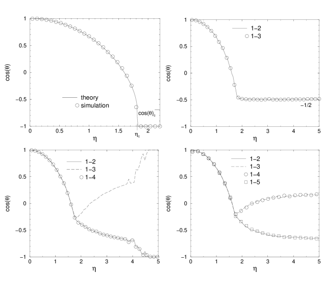
FIG. 3.: Mutual learning with rule $PN$ (cf. sections I B and I C): the system follows Eq. (10) for $\eta<\eta_{c}$. Simulations used $N=100$.

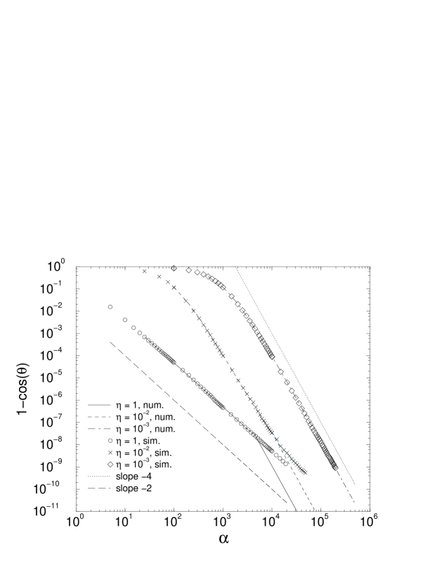
FIG. 4.: Mutual learning with rule $H$: simulations with $N=100$ show good agreement with Eqs. (13), except for very small angles $\theta$.

FIG. 5.: Competing learning aims with normalized weights: $\eta_{2}$ is set to 1 while $\eta_{1}$ is varied. The analytical curves are fixed points of Eqs. (29), (30) and (32), respectively.

FIG. 6.: Confused teacher: Even with the optimal weight function (44) the student only achieves an overlap of $\cos(\theta)=0$. Starting values are $w_{1}=w_{2}=\sqrt{2\pi}/4$, $\cos(\theta)=1$, $\eta=1$. Simulations are performed with $N=2000$; the statistical error is smaller than the size of the symbols..

FIG. 7.: Confused teacher: If the teacher is slowed down by normalizing its weight, it can be tracked by a student using e.g. rule $HN$. The figure shows the fixed point of (48) and simulations with $N=100$.

FIG. 8.: Fixed point of $C$ vs. $\eta$: simulations with $N=100$ agree well with Eq. (58). The limit for $K\rightarrow\infty$ is $C=\sqrt{2\pi}\eta/4$.

FIG. 9.: Fixed point of $\sigma^{2}/K$ vs. $\eta$: the combination of Eqs.(51) and (58) shows that sufficiently small learning rates lead to $\sigma^{2}/K<1$.

FIG. 10.: Using a modified $PN$ algorithm improves the results, compared to Fig. 9. Simulations again use $N=100$.

REFERENCES

- [1] J. Hertz, A. Krogh, and R. Palmer, Introduction to the Theory of Neural Computation (Addison-Wesley, Redwood City, 1991).
- [2] M. Opper and W. Kinzel, in Models of Neural Networks III, edited by E. Domany, J. van Hemmen, and K. Schulten (Springer Verlag, Heidelberg, 1995), Chap. Statistical Mechanics of Generalization, pp. 151–209.
- [3] On-line Learning in Neural Networks, edited by D. Saad (Cambrigde University Press, Cambridge, 1998).
- [4] M. Biehl and P. Riegler, Europhys. Lett. 28, 525 (1994).
- [5] E. Eisenstein, I. Kanter, D. Kessler, and W. Kinzel, Phys. Rev. Letters 74, 6 (1995).
- [6] M. Schröder and W. Kinzel, J. Phys. A 31, 9131 (1998).
- [7] D. H. Wolpert and K. Turner, cs.LG/9908014 (unpublished).
- [8] M. Biehl and H. Schwarze, J. Phys. A 26, 2651 (1993).
- [9] W. B. Arthur, Am. Econ. Assoc. Papers and Proc 84, 406 (1994).
- [10] D. Challet and Y.-C. Zhang, Physica A 246, 407 (1997).
-
[11]
M. Marsili, D. Challet, and R. Zecchina, cond-mat/9908480 (unpublished),
D. Challet, M. Marsili, and R. Zecchina, Phys. Rev. Lett. 84, 1824 (2000),
D. Challet and Y.-C. Zhang, Physica A 256, 514 (1998),
R. Savit, R. Manuca, and R. Riolo, Phys. Rev. Lett. 82, 2203 (1999),
D. Challet and M. Marsili, Phys. Rev. E 60, R6271 (1999). - [12] G. Reents and R. Urbanczik, Phys. Rev. Lett. 80, 5445 (1998).
- [13] H. Zhu and W. Kinzel, Neural Computation 10, 2219 (1998).
- [14] O. Kinouchi and N. Caticha, J. Phys. A 25, 6243 (1992).
- [15] D. Challet, M. Marsili, and Y.-C. Zhang, cond-mat/9909265 (unpublished).
- [16] N. F. Johnson, M. Hart, P. M. Hui, and D. Zheng, cond-mat/9910072 (unpublished).
- [17] A. Cavagna, Phys. Rev. E 59, R3783 (1999).