Kinetics of Ordering in Fluctuation-Driven First-Order Transitions: Simulations and Dynamical Renormalization

Abstract

Many systems where interactions compete with each other or with constraints are well described by a model first introduced by Brazovskii. Such systems include block copolymers, alloys with modulated phases, Rayleigh-Benard Cells and type-I superconductors. The hallmark of this model is that the fluctuation spectrum is isotropic and has a minimum at a nonzero wave vector represented by the surface of a d-dimensional hyper-sphere. It was shown by Brazovskii that the fluctuations change the free energy structure from a $\phi^{4}$ to a $\phi^{6}$ form with the disordered state metastable for all quench depths. The transition from the disordered to the periodic, lamellar structure changes from second order to first order and suggests that the dynamics is governed by nucleation. Using numerical simulations we have confirmed that the equilibrium free energy function is indeed of a $\phi^{6}$ form. A study of the dynamics, however, shows that, following a deep quench, the dynamics is described by unstable growth rather than nucleation. A dynamical calculation, based on a generalization of the Brazovskii calculations shows that the disordered state can remain unstable for a long time following the quench.

I Introduction

Kinetics of growth can be broadly classified into two categories; nucleation and spinodal decomposition (or continuous ordering). The former applies to situations where the initial state is metastable and the latter to where the initial state is unstable. The distinction becomes unclear near the limit of metastability and in systems where the concept of metastability itself is ill-defined. A class of systems where the definition of metastability becomes ambiguous is one where there is a fluctuation-driven first-order phase transition. A notable example of a system undergoing such a transition is a symmetric di-block copolymer. These systems undergo microphase separation and there is a temperature-driven transition from a uniform phase to a lamellar phase[1]. Another system which is governed by the same dynamical equation as block copolymers, and so exhibits a similar transition, is a Rayleigh-Benard Cell [2].

A theoretical model describing these transitions was proposed by Brazovskii in 1975[3]. Di-block copolymers were shown to belong to the Brazovskii class by Leibler[4] and the theoretical predictions regarding the equilibrium nature of the ordering transition have been experimentally verified[5]. It was shown by Brazovskii, within a self-consistent Hartree approximation, that the fluctuations destroy the mean-field instability and lead to a first-order phase transition[3, 6]. Theories of nucleation and growth have been constructed based on the idea that the static, Brazovskii-renormalized theory can provide an effective potential for a stochastic Langevin equation[6, 7]. In this paper we examine the validity of this description by using numerical simulations to study the relaxational dynamics of a model described by the Brazovskii Hamiltonian and comparing the results to the predictions of the “static” nucleation theories and to the predictions of a dynamically renormalized theory[8].

II The Equation of Motion and Numerical Simulations

Our starting point is the same as in Swift and Hohenberg[7] and describes a system with model A dynamics[9] and a Brazovskii Hamiltonian such as would apply to the diblock copolymers[6]. The Brazovskii Hamiltonian is characterized by a fluctuation spectrum whose maximum occurs at a non-zero wave vector $|{\bf q}|=q_{0}$ and can be represented by a hypersphere in $d-$ dimensions. The full form of the Hamiltonian is

$$H=\int d{\bf{x}}[\frac{1}{2}\phi(\nabla^{2}+q_{0}^{2})^{2}\phi+\frac{1}{2}\tau\phi^{2}+\frac{1}{4!}\lambda\phi^{4}]$$ (1)

The dynamics is taken to be relaxational and so the equation of motion is given by the Langevin Equation.

$$\frac{d\phi}{dt}=-M\frac{\delta H}{\delta\phi}+\eta$$ (2)

where $M$ is the mobility (which sets the time scale for the problem) and $\eta$ is Gaussian noise ($<\eta>=0,$ $<\eta(\vec{x},t)$ $\eta(\vec{x}^{\prime},t^{\prime})>=\delta(\vec{x}-\vec{x}^{\prime})\delta(t-t^{\prime})$ ).

The stochastic Langevin equation derived from the Hamiltonian differs from the usual Ginzburg-Landau description[9] because of the appearance of the unusual gradient term. This dynamical equation is usually referred to as the Swift-Hohenberg equation and falls into the Type $I_{s}$ classification of Cross and Hohenberg [11]. In this classification the system is unstable to a static, spatially periodic structure.

The complete equation of motion is;

$$\frac{d\phi}{dt}=-M(q_{0}^{2}\nabla^{2}\phi+\nabla^{4}\phi+(q_{0}^{4}+\tau)\phi+\frac{\lambda}{6}\phi^{3})+\eta$$ (3)

In Eq. (3), the coupling constant, $\lambda$ has been rescaled by the noise strength. For systems where the noise strength is small, such as Rayleigh-Benard convection[10], the effective coupling constant is also small. In di-block copolymers, the noise strength is of the order of $k_{B}T$.

For numerical calculations, the Langevin equation must be approximated by a discrete equation.

$$\phi(t+\Delta t)=\phi(t)-M\Delta t(\pounds\phi+\pounds^{2}\phi+(r+q_{0}^{4})\phi+\frac{\lambda}{6}\phi^{3})+(M\Delta t/(\Delta x)^{3})^{1/2}\eta$$ (4)

£ here is the discrete Laplacian. This can take on several forms though for this work we use the simplest form: $\frac{d^{2}\phi}{dx^{2}}\approx\pounds\phi=\sum\frac{1}{\Delta x^{2}}(x+\Delta x)+\phi(x-\Delta x)-2\phi(x))$ where the sum is over the dimensions of the lattice. Other choices which include next nearest or more complicated neighborhoods are possible[12]. This is important if isotropy is of concern however the effect is small and can be ignored. The scaling of the noise in Eq. 4 reflects the fact that as the cell size or time steps become smaller (larger), the possible fluctuations become larger (smaller).

For these simulations we set $q_{0}=1$ and choose the lattice spacing such that one lamellar spacing spans six lattice sites ($\Delta x=6/2\pi$) For most of this work the overall lattice size is $60^{3}$. The mobility, $M$, is set to one. In order for the simulations to be numerically stable the time scale must be smaller then some stability time, $\Delta t\sim 1/\Delta x^{4}.$ To satisfy this the timescale is chosen to be $\Delta t$ = 0.01 and measurements are taken at intervals of $100*\Delta t$ or longer.

Previous theories of nucleation have analyzed the above equation under the approximation that the effects of fluctuations can be incorporated into a static renormalized free energy $F_{R}$ which replaces the bare free energy $F$ in Eq. (2) [6, 7]. We will compare our numerical results to the Brazovskii predictions for the static renormalized parameters and show that the static scenario is beautifully borne out by the simulations in three dimensions. We will then analyze the time-dependence of the structure factor as observed in the numerical simulations and show that this time dependence is inconsistent with the dynamical picture based on a static renormalized free energy. A theory based on a dynamical renormalization of Eq. (2) can provide a qualitatively correct description of the numerical simulations.

III Statics

A Brazovskii Theory

Brazovski’s treatment of the model within the Hartree approximation can be restated in terms of an expansion of the thermodynamic potential $\Gamma(\bar{\phi})$, the generating functional for the vertex functions[13, 14]. This approach has been described in detail by Fredrickson and Binder[6], and within the Hartree approximation leads to a renormalized mass term ($r$) in Eq.(1). The diagrams up to one loop are shown in Fig. 1, and the mass renormalization relation is given by;

$$r+(q^{2}-q_{0}^{2})^{2}=\tau+(q^{2}-q_{0}^{2})^{2}+{{\frac{\lambda}{2}}}\int{{\frac{d{\bf q}}{(2\pi)^{d}}}}(\tau+(q^{2}-q_{0}^{2})^{2})^{-1}$$ (5)

This approximation is made self consistent by replacing the bare parameter in the integrand by the renormalized parameter. Essentially the bare propagator on the loop in Fig. (1) is replaced by renormalized propagator. The leads to the Hartree result.

$$r=\tau+{{\frac{\lambda}{2}}}\int{{\frac{d{\bf q}}{(2\pi)^{d}}}}(r+(q^{2}-q_{0}^{2})^{2})^{-1}=\tau+\alpha\lambda/\sqrt{r}$$ (6)

where $\alpha$ is proportional to the surface area of a $d$ dimensional sphere of unit radius. According to Brazovski[3] this approximation is good only for $\lambda^{-6}<<1.$

The interesting point about Eq. (6) is that even for negative values of the bare parameter, $\tau$, the renormalized parameter, $r$, is positive. This implies that the disordered phase is always metastable. Brazovskii went on to show that the bare coupling parameter $\lambda$ gets renormalized to a negative value leading to a $\phi^{6}$ theory and the possibility of a first-order phase transition[6].

B Computational Results.

The numerical simulations can measure the static structure factor in the disordered phase which is predicted by the Brazovskii theory [3, 6] to be,

$$S(q)^{-1}=r+(q^{2}-q_{0}^{2})^{2}$$ (7)

where $r$ is the renormalized control parameter [3, 7]. Thus, $S(q_{0})^{-1}$ is just $r$. The renormalized mass can, therefore, be measured by monitoring the peak of the structure factor. The Hartree calculations predict $r$ to be positive and asymptotically approaching zero as $\tau\rightarrow-\infty$. Experiments in symmetric di-block copolymers have verified that the behavior of $S(q_{0})$ is consistent with the Brazovskii predictions and is very different from the mean-field prediction ( $S(q_{0})=\tau^{-1}$).

Fig. 2 shows results for $r$ obtained from our simulations for different values of the coupling constant, $\lambda$. The Gaussian case ($\lambda=0$) is also shown for comparison. The system was run for 1000 time steps (each time step being $100*\Delta t$) and 100 samples were taken. The data points plotted are the average of the samples while the error bars represent the standard deviation. For large positive values of the bare control parameter, $\tau$, the fourth order term becomes less important and $r$ approaches the Gaussian value. This is seen clearly for small values of $\lambda$. As $\tau$ approaches zero, the measured values of $r$ deviate from the Gaussian case and stay positive for all $\tau$. Some care was taken to normalize the values presented in Fig. 2. For the Gaussian case, $S(q_{0})^{-1}$ should be linearly related to $\tau$ and the slope of the line should be one. In calculating $S(q_{0})$ several normalizations are needed including the normalization due to the Fourier Transform (FT) and the normalization due to circular averaging. While the FT normalization is just related to the system size, the normalization due to circular averaging is more complicated to calculate. Instead of calculating these normalizations directly, the slope of the raw result from the Gaussian case was used to normalize all of the data. Another concern is that for an infinite continuous system this line should have an x-intercept at zero; however, for the finite systems on a grid used in the simulations the x-intercept is slightly negative. To account for this, all of the data is shifted over by an amount equal to that intercept. The importance of this shift will become apparent in the next paragraph when a scaling is applied and the values of the results around zero are magnified. A small negative (positive) value becomes a much larger negative (positive) value and so shifts from negative to positive will become important.

In reference[7] the authors show that, within the Hartree approximation, the $r(\tau)$curves for different $\lambda^{\prime}s$ could be described by a single functional form in terms of scaled variables $\tau^{*}$ and $r^{*}$;

$$r^{*} = r*(\alpha\lambda)^{-2/3}$$ (8)

$$\tau^{*} = \tau*(\alpha\lambda)^{-2/3}$$ (9)

Figure 2 shows plots of $r^{*}$ against $\tau^{*}$obtained from simulations for the three different values of $\lambda$. The curves are seen to scale quite well but the scaled curve falls significantly below the theoretical prediction [3, 6, 7] shown as the thick black line. The theoretical prediction that the value of $r^{*}$(and $r$) never becomes negative and is asymptotic to zero is, however, clearly borne out by the simulations. The deviation from the theoretical line could be a system size effect, however, results for larger and smaller systems are consistent with the data shown in Fig.3. For the Gaussian case $r^{*}=\tau^{*}$ and for large positive values of the bare parameter both the theory and simulations approach this. Since the theory is larger then the simulations and both are above the Gaussian, our simulations suggest that the contributions to the two point function from diagrams not included in the Hartree approximation serve to lower the overall correction to mean field theory. Another property that the simulation data exhibits in Fig. 3 which is not predicted by the theory is that the curves for different values of $\lambda$ diverge from each other at negative values of $\tau$, i.e. the scaling is not perfect. Smaller values of $\lambda$ lie closer to the theory as expected. The computations were done using values of $\lambda\sim 10^{-2}$ and larger while the theory is valid only for $\lambda\sim 10^{-6}$ so the theory’s scaling predictions seem to be far more robust then expected.

To further explore the nature of the phase transition in this model, we can compare scaled values of $S(q_{0})$ obtained from a hot (random) and cold (purely modulated order) initial configurations. Fig. 4 shows just such a plot. As in the previous plot, the theory is shown as a thick black line. For each value of $\lambda$ there are two lines presented: one for a disordered start and one for an ordered start. The averaging was done as described above. For positive and small negative values of $\tau$ the results from the disordered start and the ordered start are nearly the same. For $\tau^{*}$ below some $\tau_{s}^{*}$ the two differ with the ordered phase having a higher peak. It should be pointed out that for these values of $\tau^{*}$ the disordered state is not in equilibrium (metastable or stable)and there is a slow but definite time evolution of the structure factor over the time period in which the averages are taken. This time-evolution will be discussed in more detail in the section on dynamics. For now the disordered start points are included in the plot simply as a comparison to see where the ordered phase melts. The value where the two data sets diverge can be considered an estimate for the limit of stability (spinodal) of the lamellar phase. As a consistency check the average value of the wave vector was measured. For values of $\tau$ above $\tau_{s}$ the wave vector is small and points in a random direction, while for lower values of $\tau$ the average wave vector is large and and points along the direction that the system was prepared in. For all three sets of data the lamellar spinodal lies in the range of $-2.1<\tau_{s}^{*}<-1.9$. This is consistent with the prediction from Hartree theory that the first-order transition to the lamellar phase occurs at a lower value of $\tau^{*}$, ${\tau}_{t}^{*}=-2.74$[7]. That is to say that our measured value of the lamellar spinodal is above the predicted transition temperature as it should be. For values of $\tau^{*}$ below $\tau_{s}^{*}$, however, systems prepared in the disordered phase always evolve towards the ordered phase. It is possible that the lamellar ordered phase is enhanced by the boundary conditions - the lattice size is always chosen to be commensurate with the lamellar wavelength - however, it should be noted that lamella form in many possible directions where the system size is not commensurate with the lamellar wavelength. Discussion in the dynamics sections should shed some light on this issue.

IV Dynamics

A Relaxational Dynamics Based on Static Renormalized Parameters

Previous analysis of nucleation and metastability, in the context of fluctuation-driven phase transitions, have been based on a Langevin equation with the force obtained from the static, Hartree-renormalized free energy function[6, 7]. Fredrickson and Binder[6] used this approach to compute the nucleation barrier and the completion rate of nucleation and growth in di-block copolymers. The interfacial tension was found to be small leading to a small nucleation barrier and rapid nucleation for deep quenches. In this picture, there is no essential difference between the kinetics of a fluctuation-driven first-order transition and a weak-first order transition. The results of our simulations suggest a very different scenario for the growth of the lamellar structures in a Brazovskii model. The shape of the nucleating droplet was more carefully analyzed by Swift and Hohenberg[7] by taking into account spatial inhomogeneities in the effective free energy function. Their analysis relied on constructing a coarse-grained free energy functional. The coarse graining was based on a momentum-shell renormalization idea where fluctuations with momenta far away from the shell defined by $|{\bf q|=q_{0}}$ are successively integrated out. This analysis led to non-spherical droplets and were consistent with the picture of spinodal nucleation that had been obtained earlier[15].

As pointed out in the work of Swift and Hohenberg[7], a complete theory of the dynamics of fluctuation-driven first order transitions would have to be based on a coarse-graining of the full dynamics as expressed by the original Langevin equation with the bare Brazovskii Hamiltonian. In this paper, we compare the results of our numerical simulations to the predictions of a Hartree-renormalization of the full dynamical equation as expressed in Eq. (2). Our emphasis has been on understanding the nature of the dynamics of the metastable phase and we have not analyzed, in any detail, the spatial structures associated with the growth process.

B Dynamical Renormalization and Simulation Results

In order to systematically analyze the effects of fluctuations on the kinetics of growth of the lamellar phase, perturbative techniques analogous to the static Hartree approximation have to be applied to the Langevin equation. This is most conveniently done through the dynamical-action formalism[14]. The application of this method to the S-H equation is outlined by Ignatiev et. al. [8]. In the dynamical-action formalism, the average value of an operator $O(\phi)$ over the noise history is rewritten as a functional integral;

$$\langle O\{\phi({\bf x},t)\}\rangle=\int D{\phi}\exp{(-S[{\phi}])}~{},$$ (10)

where $S[{\phi}]$ is the dynamical action[14].

As in the static case, the calculation of dynamical correlation functions is most conveniently formulated through the construction of a generating function[14, 13]. To establish the closest analogy with the static calculations, it is useful to work with the generator of vertex functions, ${\ \ \ \Gamma}_{dyn}[\bar{\phi}]$, and establish a diagrammatic expansion which is the exact analog of the diagrams retained by Brazovskii in the static calculation. The simulation results demonstrate that the static properties of the S-H equation closely follow the Brazovskii predictions and, therefore, it seems appropriate to apply this approximation scheme to the dynamics. The correspondence between statics and dynamics becomes particularly transparent in a super-field formulation[16] which shows that the dynamical perturbation theory in terms of the super fields has exactly the same structure as the static perturbation theory except for the appearance of a very different “kinetic” term which leads to a bare propagator that is distinct from the static theory. The super-field correlation functions can be calculated by constructing diagrams as in the static theory but replacing the static bare propagator by the appropriate dynamical one[16]. The super-field correlation functions encode all the dynamical correlations of the field $\phi$ and the latter can be extracted from well-defined relations[16]. The details of this calculation and the results will be described in a separate publication[8]. In this paper we present the main results which can be compared to the numerical simulations.

The two correlation functions which appear in the dynamical study are

$\displaystyle G(t,t^{\prime})=<\phi(t)\eta(t^{\prime})>$

and

$\displaystyle C(t,t^{\prime})=<\phi(t)\phi(t^{\prime})>$

Both of these can be obtained from a single super-field correlation function ($Q(1,2)$) which is related to $\Gamma_{dyn}$ through

$$Q^{-1}(1,2)={\frac{{\delta}^{2}\Gamma_{dyn}}{\delta\Phi_{1}\delta\Phi_{2}}}$$ (11)

where $\Phi$’s are the super fields and the derivative is evaluated with the source term set to zero. Applying this formalism to Eq. (2), leads to an expression for $\Gamma_{dyn}$ which involves two-point correlation functions of the fluctuations and is a natural extension of the static $\Gamma(\bar{\phi})$ to correlation functions involving time. The expression, however, does not lend itself to easy analysis except in two cases, early times when a variant of linear theory can be applied and late times when the system is stationary. The late time dynamics involves the analysis of the nonlinear terms and will be discussed in the concluding section. The early time dynamics is where one is justified in retaining only quadratic terms in the renormalized $\Gamma_{dyn}$. In this limit we obtain the following equation for the equal-time correlation function $C_{q}(t,t)=<\phi_{q}(t)\phi_{-q}(t)>$ which is the structure factor that is monitored in the simulations:

$$C_{q}(t,t) = {\int}_{0}^{t}[G(t,t^{\prime})]^{2}dt^{\prime}$$ (12)

$$G_{q}(t,t^{\prime}) = \int_{t}^{t^{\prime}}(r(t^{\prime\prime})+(q^{2}-q_{0}^{2})^{2})dt^{\prime\prime}~{}.$$ (13)

The mass parameter, $r(t)$, which is now time-dependent, is renormalized in the dynamic theory using the same approximation as in the static theory. The diagrams used are given in fig. 7. These again are only to one loop. The mass term then becomes

$$r(t)+(q^{2}-q_{0}^{2})^{2} = \tau+(q^{2}-q_{0}^{2})^{2}+$$ (15)

$${{\frac{\lambda}{2}}}[\int{{\frac{d{\bf q}}{(2\pi)^{d}}}}\frac{1}{(\tau+(q^{2}-q_{0}^{2})^{2})}-\int{{\frac{d{\bf q}}{(2\pi)^{d}}}}\frac{\exp\{-2(\tau+(q^{2}-q_{0}^{2})^{2})t\}}{(\tau+(q^{2}-q_{0}^{2})^{2})}]$$

Again, the approximation is made self consistent by replacing the $\tau$ with $r$ in the integrand.

$$r(t)=r_{eq}-{{\frac{\lambda}{2}}}\int{{\frac{d^{3}q}{(2\pi)^{3}}\frac{\exp(-2D(q)t)}{D(q)}}}$$ (16)

$D(q)$ here is the renormalized propagator, $D(q)=r_{eq}+(q^{2}-q_{0}^{2})^{2}$ where $r_{eq}$ denotes the static renormalized mass parameter which is the solution to eq. 7.

In Eq. 16, at long times the integrand in the second term becomes small and $r(t)$ approaches $r_{eq}.$ which is confirmed in the section on statics above. At time zero the subtraction of the second term is just a subtraction of the Hartree level correction factor to the bare parameter introduced earlier Eq. (6 and, therefore, $r(t=0)$ is just the bare parameter $\tau$, while as $t\rightarrow\infty$, $r(t)$ approaches the renormalized, equilibrium value.

This scenario is confirmed by the simulations. The simulation results discussed in Section III B confirm that the equilibrium value, $r_{eq}$, is consistent with the Hartree prediction. Analyzing the early stage dynamics can verify the value of $r(t)$ at short times. Figure 5 shows the growth of $S(q_{0})$ as a function of time for various values of the bare control parameter, $\tau$. To average over noise, five independent runs where taken for each value of the control parameter. If $r(t)$ is time-independent, the early-stage evolution (linear theory) is described by [17]

$$S(q,t)=C_{q}(t,t)=S(q,0)\exp\{-D(q)t\}+{\frac{1}{D(q)}}(1-\exp\{-D(q)t\})$$ (17)

where $D(q)$ is $D(q)=r_{0}+(q^{2}-q_{0}^{2})^{2}$ and $r_{0}$ is the time-independent value of $r$. At the peak of the structure factor, $q=q_{0}$ , and $D(q_{0})$ is just $r_{0}$, the value of which can be estimated by fitting the simulation results shown in Fig. 5 to 17. The results of such fits are presented in Fig. 6. This figure shows that $r_{0}$ and $\tau$ are linearly related with a slope which is nearly one. This implies that for short times, the dynamically renormalized parameter is linearly related to the bare parameter and is not renormalized to positive values for negative values of the bare parameter. The very early-stage dynamics, therefore, is characteristic of a system exhibiting unstable growth.

These fits must be considered with some care. In the case where $r$ is not time dependent, the linear theory describes the system only for short times, that is times on the order of the natural time scale, $r^{-1}$ [See for example[18]. For the fastest growing mode, when the data is fit to different time scales the results obtained are consistent for all time scales up to $r^{-1}$. For the S-H equation, however, the results obtained are dependent on the time range. In particular, as the range of time increases the values obtained for $r$ become less negative. This is consistent with $r(t)$ growing as a function of time and the results of the fits merely represent some average value of $r(t)$ for the time range involved. If the system has been quenched to a negative value of $\tau$, Eq. 16 indicates that the early-time evolution will exhibit unstable growth. As time evolves the second term in Eq. (16) decreases and the value of $r(t)$ approaches $r_{eq}$ which is always positive. Though the integral in Eq. 16 is hard to evaluate analytically, numerics can provide some insight into its behavior. Figure 8 shows a numerical evaluation of the time evolution of $r(t)$ for various values of $r_{eq}$ and $\lambda=0.01$. As confirmed in the statics section above, $r(t)$ will eventually become positive no matter how deep the quench is, though the time for this to happen may become very long. As long as $r(t)$ is negative the system is expected to undergo unstable growth though, since the mass parameter is time-dependent, the time evolution will be more complicated than the usual spinodal decomposition scenario. We can define a crossover time, $t_{cross}$ at which $r(t)$ changes sign, and an average growth time, $t_{ave}$. The average growth time is just the inverse of $r_{ave}$ defined as

$$t_{ave}^{-1}=r_{ave}=\frac{1}{t_{cross}}\int_{0}^{t_{cross}}r(t^{\prime})dt^{\prime}$$ (18)

In Fig. 9, we show plots of $t_{cross}$ and $t_{ave}$ as a function of the bare control parameter. For shallow quenches $t_{cross}$ is small compared to $t_{ave}$ and the system reaches a well-defined metastable equilibrium state which is disordered. If $t_{cross}$ becomes larger then $t_{ave}$, metastability becomes difficult to define. The system takes longer to equilibrate in the metastable disordered phase than it takes to grow lamellar structures. We can use the condition $t_{cross}=t_{ave}$ to define a crossover temperature ${\tau}_{dyn}^{*}$. Above this temperature the disordered phase quickly becomes locally stable and a nucleation event is needed for the formation of the lamellar structures. Below ${\tau}_{dyn}^{*}$, the system is expected to evolve continuously towards the lamellar phase without any evidence of metastability of the disordered phase. Fig. 9 is in sharp contrast to standard Ginzburg-Landau (G-L) theory. For the time dependent G-L equation, the presence of noise suppresses the critical point. In the region where the bare parameter is negative but the renormalized parameter is positive, $t_{cross}$ is always smaller then $t_{ave}$ and so there is no unstable growth until the true critical point is reached.

For the system under consideration here, different scenarios are possible depending on the relationship of this dynamical crossover temperature to the first-order transition temperature, ${\tau}_{trans}^{*}$ , at which the free energy of the lamellar phase becomes lower that that of the disordered phase. If ${\tau}_{trans}^{*}$ is higher than ${\tau}_{dyn}^{*}$, there will be a regime of temperatures over which the the system will undergo nucleation and growth. On the other hand if ${\tau}_{trans}^{*}$ is lower than ${\tau}_{dyn}^{*}$, then there is no nucleating regime and one would observe only unstable growth, albeit of an unusual nature since the free-energy surface is evolving with time. From figure 9 we can see that $t_{cross}$ is small only for very shallow quenches below the mean-field transition. The results of our simulations, presented in the next section, are in qualitative agreement with this scenario. We would like to emphasize that the growth dynamics described above are qualitatively different from rapid nucleation in which the system quickly reaches the stable equilibrium state. A large value of $t_{cross}$, on the other hand, indicates a type of ergodicity breaking as the system takes a very long time to reach equilibrium.

All of our numerical results indicate that ${\tau}_{trans}^{*}$ predicted from Hartree is lower than ${\tau}_{dyn}^{*}$ and they are remarkably close to each other. We have been unable to come up with a simple relationship between these two temperatures and, therefore, can only interpret the similarity of the two as a remarkable coincidence. The dynamical crossover is deduced from time scales which characterize the evolution of the free-energy surface while the transition temperature is deduced from a comparison of the depth of the two wells. It is not clear why the two temperatures should be similar in magnitude. It can be argued that there is only a single parameter, $\lambda$, controlling the scale of fluctuations and, therefore, the two temperatures should be related, however, there is no obvious argument to suggest that they should be identical.

The picture emerging from the dynamical renormalization is a natural extension of the effect of fluctuations on the static results of the Brazovskii model. Following a quench from a relatively high temperature to a temperature where $\tau$ is negative, the system is in a locally unstable region (top of a hill). As the fluctuations grow with time, the non-linear terms characterized by $\lambda$ become important and they renormalize the curvature of the hill. This scenario is quite different from the usual picture of evolution in an adiabatic potential.

C Simulation Results for Late Times

Further evidence for the dynamical scenario presented in the previous section comes from examining the long time evolution of the peak of the structure factor obtained from our numerical simulations and correlating that to snap shots of the system as it evolves. Figure 10 is a plot of the amplitude of the structure factor peak as it evolves. For shallow quenches, $\tau>-0.04,$the peak grows to an equilibrium value and does not evolve further. These values are consistent with the equilibrium values reported above in the section on statics. For deeper quenches the peak amplitude grows quickly and then appears to saturate; however careful examination shows that the value continues to grow very slowly. This is consistent with late stage domain growth which as been studied extensively by Elder et. al. for 2-D systems [22]. The last feature in the system is a final rise to an equilibrium value. This rise is a finite size affect is caused by the majority domain finally taking over the entire system. This being the case, the peak would not be expected to grow much since the difference between the value before and after this final evolution should only represent the surface area between the different domains.

For a quench depth of $\tau=-0.07$ this time evolution can be compared to a series of system snapshots shown in figures 11- 15. These figures represent $\phi=0$ isosurfaces which would be the boundaries between the different microphases of the system. For early times the system appears to be very disordered while at later times domains of ordered lamellar structures begin to appear. Just before the final convulsive growth, at a time $t=4000$, there still appear to be a few different ordered domains while just after the final growth, at $t=5000$, only one domain appears to be left in the system. Thus we still have a consistent picture of slow but continuous domain growth in the system which is governed by the evolution of the 2nd order term as it goes from negative values to positive values.

V Future Work

In the work presented above we have shown that analysis of the static free energy does not always provide an adequate description of the fluctuation driven dynamics. Though figure 10 shows features which are reminiscent of a first order phase transition, dynamical analysis of the renormalized coefficients suggest that a more complicated evolution is taking place. A similar situation occurs for the superconducting transition which is also a fluctuation-driven first-order transition[19].

In the present work we have paid close attention to the time evolution of the mass parameter and its effect on the evolution of the system at early times. The dynamical renormalization results also become tractable at times large compared to $t_{cross}$ when the system has reached equilibrium. As pointed out earlier, one enters this regime fairly quickly for shallow quenches. At this stage, the higher order terms in $\Gamma_{dyn}$ become important. The most interesting aspect of the renormalized theory is that the fourth-order term becomes non-local in time [8]:

$\displaystyle\Gamma_{dyn}(4)\simeq\int d1d2\Phi^{2}(1)K(1-2)\Phi^{2}(2)$

and the integral of the kernel over all times leads to the Brazovskii result for the renormalized fourth-order term. One can derive an “effective” Langevin equation for the fields $\phi$ from the renormalized $\Gamma_{dyn}$, and the above equation implies that this Langevin equation has “memory” effects which appear in the non-linear term. This would lead to unusual behavior of the equilibrium correlations functions and might provide a distinctive signature of fluctuation-driven first-order transitions. We are in the process of investigating the effective equation for $\phi$ numerically. One obvious consequence of the non-local term is that the barrier to nucleation is dynamic and it is not valid to think of nucleation as tunneling through a fixed barrier. The situation is closer to the problem of quantum tunneling for many degrees of freedom where one also finds an effective equation which is non-local in time[20].

Another area of interest is the role of defects in the phase transition of the system. These will be important for very shallow quenches to just below the transition point and we have noted there presence when looking at snapshots of the system. These defects are reminiscent of the perforated lamellar phase described in reference [1]. One way to study this is to use a directional order parameter measure introduced by Bray et al.[21] to study the 2D problem. This order parameter is similar to the order parameter for complex fluids and provides directional as well as density information. What it may show is that the local gradient terms are enhanced for negative values $\tau$ suggesting that perhaps there is a disordered to nematic transition in this region which others have suggested for 2D [22].

We would like to close with a discussion of possible experimental systems where this dynamical scenario can be studied experimentally. Since the effective $\lambda$ is extremely small in Rayleigh-Benard systems the regime where the disordered state is metastable will probably be unaccessible. In di-block copolymers, however, there should be a significant temperature range, below the mean-field transition, where the disordered state is locally stable and a study of the equilibrium, two-time correlation function should reveal the existence of the non-linear memory term. It might also be possible to observe unusual nucleation if the system parameters allow for $\tau_{trans}^{*}$ to be higher than $\tau_{dyn}^{*}$.

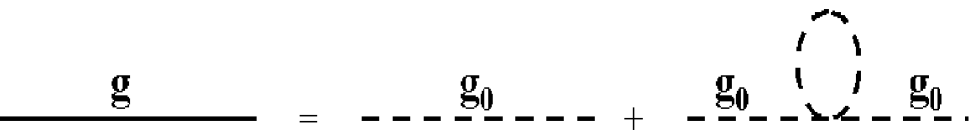
FIG. 1.: Diagrams used for static renormalization of the mass parameter in the free energy. The Hartree approximation only uses diagrams up to order $\lambda$ and then replaces the bare parameter in the integrand with the renormalized one to solve the equations self consistently.

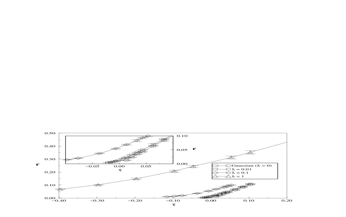
FIG. 2.: The renormalized control parameter, $r$, against the bare control parameter, $\tau$. The different data sets are for different values of $\lambda$. The Gaussian case, $\lambda=0,$ which was used to set the scale, is also plotted for comparison. The inset shows the region near the mean field transition. Note that the renormalized parameter does not cross zero here.

FIG. 3.: Scaling of $r(\tau)$ using the form deduced from Hartree theory (cf text). The data collapses well except at the deepest quenches. The scaling curve predicted by the Hartree approximation is shown for comparison. It is in fairly good agreement with the data considering that the values of $\lambda$ used in the simulations are four order of magnitude larger then that for which the the approximation is expected to be valid.

FIG. 4.: Temperature dependence of the average intensity at the peak of the structure factor. To show the transition, results from two different starting configurations are compared. The shapes of the symbols denote different values of $\lambda$, whereas the shading distinguishes between the starting configurations. The closed symbols represent systems that were started in a disordered state, simulating a hot start, while the open symbols are for systems which were started with an ordered lamellar structure already present. At high temperatures the two starting conditions give nearly the same results while at low temperatures the systems prepared in the ordered state have higher peak intensities implying that the systems prepared in the disordered states are in a metastable state or not in equilibrium (cf text).

FIG. 5.: The time evolution of the structure factor peak for the earliest times. Different sets are for different quench depths as indicated on the graph. All quenches to below the mean field transition temperature initially show unstable growth.

FIG. 6.: Growth time as calculated from fits to a linear theory plotted against the quench depth below the mean field transition. For short times the system should be described by linear theory which predicts unstable growth for all quenches below the mean field transition.

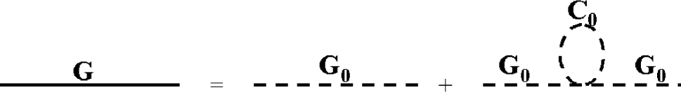
FIG. 7.: As with the static case, diagrams only up to order $\lambda$ are used and then the bare parameter is replaced by the renormalized parameter to give a self consistent solution.

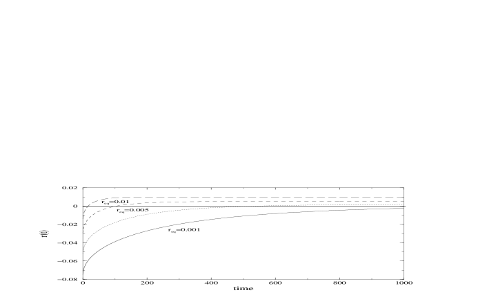
FIG. 8.: The time evolution of the mass parameter as calculated by dynamic renormalization. $r(t)$ eventually becomes positive for all quenches below the mean field transition but the time for that cross over increases dramatically for larger quenches. At large times $r(t)$ approaches $r_{eq}$.

FIG. 9.: The calculated crossover time plotted against quench depth. Also plotted is a characteristic growth time for the lamellar structure. These results have been scaled using equation 8 so that they are $\lambda$-independent. When this time becomes much less then the crossover time then the lamella has enough time to grow. Notice that this occurs just above or at the transition temperature, ${\tau}_{trans}$.

FIG. 10.: The evolution of the structure factor peak as a function of time for different quench depths. For shallow quenches above the real transition temperature $S(q_{0})$ grows quickly to its equilibrium value. For quenches to below the transition temperature the system grows quickly at early times and then reaches a late stage regime where it evolves by domain growth and $S(q_{0})$ grows as a small power law in time. The highlighted line is a quench to $r=-0.07$. Snapshots of this system are presented in the next figure.

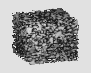
FIG. 11.: Time = 1000

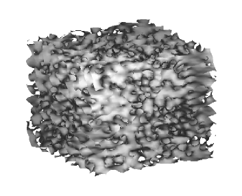
FIG. 12.: Time = 2000

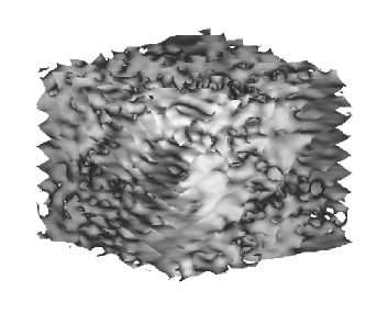
FIG. 13.: Time = 3000

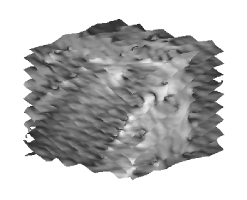
FIG. 14.: Time = 4000

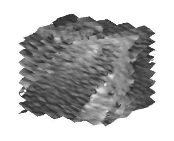
FIG. 15.: Time = 5000

REFERENCES

- [1] F. Bates and G. Fredrickson, Physics Today , 52 32 (Feb. 1999)
- [2] G. Ahler, to be published in Rev. Mod. Phys. (2000)
- [3] S.A. Brazovskii, Sov. Phys.-JETP 41 85(1974)
- [4] L. Leibler, MacroMolecules, 16 1602 (Nov.-Dec. 1980)
- [5] F. S. Bates, J. H. Rosedale and G.H. Fredrickson, J. Chem. Phys., 92, 6255 (1990).
- [6] G. Fredrickson and K. Binder, J. Chem. Phys., 91 7265 (1989)
- [7] P.C. Hohenberg and J.B. Swift, Phys. Rev. E, 52 1828 (1995)
- [8] M. Ignatiev, B. Chakraborty and N. A. Gross, in preparation
- [9] P.C. Hohenberg and B.I. Halperin, Rev. Mod. Phys. 49 435 (1977)
- [10] P.C. Hohenberg and J.B. Swift, Phys. Rev. A,46 4773 (October 15, 1992)
- [11] M.C. Cross and P.C. Hohenberg, Rev. Mod. Phys. 65 851 (1993)
- [12] Y. Oono and S. Puri, Physical Review Letters 58 836 (1987)
- [13] Daniel J. Amit, Field Theory, the Renormalization Group, and Critical Phenomena, (World Scientific, Singapore, 1997)
- [14] J. Zinn-Justin,Quantum Field Theory and Critical Phenomena, (Oxford, England, 1989)
- [15] C. Unger and W. Klein, Phys. Rev. B 29 2698 (1984)
- [16] J.P. Bouchaud, L. Cugliandolo, J. Kurchan and M. Mézard, Physica A, 226 223 (1996)
- [17] J.W. Cahn and J.E. Hilliard, J.Chem. Phys., 31, 688 (1959); H.E. Cook, Acta Metall., 18, 297 (1970)
- [18] N. A. Gross, W. Klein and K. Ludwig, Phys. Rev. E, 56, 5160(1997)
- [19] F. Liu, M. Mondello and N. Goldenfeld, Phys. Rev. Let. 66 3071 (1991)
- [20] J. Sethna, Phys. Rev. B, 24 698 (1981); B. Chakraborty, P. Hedegård and Mats Nylen, J. Phys. C., 21 3437 (1988)
- [21] J.J. Christensen and A.J. Bray, Phys. Rev. E, 58 5364 (1998)
- [22] K.R. Elder, J. Viñals and M. Grant, Phys. Rev. A 46 7618 (1992).