Statistical characterization of the fixed income market efficiency

Abstract

We present cross and time series analysis of price fluctuations in the U.S. Treasury fixed income market. By means of techniques borrowed from statistical physics we show that the correlation among bonds depends strongly on the maturity and bonds’ price increments do not fulfill the random walk hyphoteses.

, , ,

The individual evolution of complex systems can be tantalizingly difficult to describe. However, when appropriate statistical averages are taken, some form of structural regularity may be observed, that can be used to model the behavior of the system.

It so happens that the same mathematical techniques are applied to analyze widely disparate phenomena, such as fluid turbulence and the price fluctuations in the financial markets. Recently, for instance, typical concepts of statistical mechanics, such as scaling, (multi)-fractality, percolation and others are starting to play a significant role in the quantitative analysis of the behavior of financial markets.

Actually, fixed-income (FI) markets have received less attention than stock markets in terms of a quantitative characterization as a stochastic process. On the other hand, FI markets (specifically US Treasury securities markets, which is the one we are interested in) are much less volatile than stock markets since their own characteristics, in a strong-economics country with low inflation, prevent the occurrence of wild fluctuations.

Fixed income markets are expected to honor the so called “one-price law” stating that two portfolios of fixed-income securities that guarantee the investor the same cash-flows and give her the same future liabilities, must sell for the same price. If any violation of that constraint should occur, then a profitable and risk-less investment opportunity, called an arbitrage, would arise. But in an efficient market [1] such an opportunity can not last long, because as investors detect and take advantage of it, a price change occurs which re-absorbs the initial anomaly.

Note that, although not limited to FI securities (it represents, for instance the basis of the well-known Black and Scholes option pricing model), the one-price law is somehow more “natural” for such assets since the market is much more homogeneous and (for all practical purposes) default risk-free.

It is apparent that, as a consequence of the one-price law, we can expect strong correlations among bonds. In particular when a replicating portfolio exists. By “replicating portfolio” of a given bond, we mean a portfolio of bonds which assures the same cash-flow of the original one.

However, even if the price variations of the bonds are strongly correlated, so that we can consider the bond dynamics as a collective motion, the process of price evolution is not known.

The statistical characterization of such process, and the study of the link between the bonds is by no means of negligible importance, given that FI markets exceed stock markets in terms of volume liquidity. This is one of the motivations of this Letter.

We have analyzed 100 US Treasury notes and bonds in the period between 30/01/97 and 28/09/99 (694 daily prices). In [2] we focused on “cross-section” data (i.e., for a given day, the set of the prices of all Treasury securities outstanding that day) looking for arbitrage opportunities. We found that in the range of maturities 5-7 years there was a difference of (about) one percent in the price of a bond and its replicating portfolio. For longer maturities (in the range 7-30 years) it was not possible to build a replicating portfolio so it was meaningless to test the existence of arbitrage opportunities.

The aim of the present work is twofold: to investigate the consequence of the one-price law on the cross correlations and to test the random walk hyphoteses for the time evolution of the price fluctuations.

As a starting point, we build the correlation matrix and then classify the bonds according to a suitable metric.

The correlations between the price dynamics of different assets is of paramount importance in the analysis of financial markets. For instance for building multi-factor pricing models it is necessary to verify some properties of the time-series of returns.

In our case the assets are a set of FI securities $B_{i},\;i=1\ldots N$ ($N=100$) and the correlation matrix elements are defined as:

$$C_{ij}=\frac{\langle r_{i}(t)r_{j}(t)\rangle-\langle r_{i}(t)\rangle\langle r_{j}(t)\rangle}{\sqrt{(\langle r_{i}(t)^{2}\rangle-\langle r_{i}(t)\rangle^{2})(\langle r_{j}(t)^{2}\rangle-\langle r_{j}(t)\rangle^{2})}}\,\,,$$

where $r_{i}(t)\equiv\ln(p_{i}(t)/p_{i}(t-1))$ is the return, that is the logarithmic price change of the $i$-th asset between $t-1$ and $t$, and $\langle f(t)\rangle$ denotes the time average $1/T\cdot\sum_{t=1}^{T}f(t)$ (T is the sample length).

By definition $C_{ij}=0$ if bonds $i$ and $j$ are totally uncorrelated, whereas $C_{ij}=\pm 1$ in case of perfect correlation/anti-correlation.

$C$ is a $N\times N$ symmetric matrix with $1$ in the diagonal. In our data set $C_{ij}$ is positive for each pair of assets. This means that, on average, the price increments of U.S. Treasury securities have the same sign. This is not surprising since the prices of FI securities issued by a single large issuer like the US Department of Treasury depend on the same macroeconomics factors like the market expectations on future base interest rate.

The $T$ values of the logarithmic price increments can be interpreted as the coordinates in a ${\mathrm{I\!R}}^{T}$ space . A “natural” Euclidean distance exists for such space, however, following  [3], $C_{ij}$ can be used to define a different metric by means of the following simple formula:

$$d(i,j)=\sqrt{2(1-C_{ij})}\,\,.$$ (1)

This metric has the advantage that just the correlation between assets matters. The “absolute” distance of two assets becomes irrelevant as it is from a financial viewpoint.

Function (1) fulfills all the three axioms of a distance: $d(i,j)=0\Leftrightarrow i=j$, $d(i,j)=d(j,i)$ and $d(i,j)\leq d(i,k)+d(k,j)$ when restricted to the set of time series of assets with zero mean and variance equal to one. The theoretical range of the distance is $[0,2]$, but, since $C_{ij}>0$ for our data, we have $0\leq\delta\leq\sqrt{2}$.

Equipped with this distance we study the topological arrangement of the bonds. However we did not follow the approach of [3] that starts from the minimum spanning tree connecting the assets of the portfolio.

By means of an invasion-percolation algorithm, which groups together bonds whose distance falls within a threshold $\delta$, we analyze the structure of the clusters as a function of $\delta$. A bond $b_{i}$ belongs to a cluster if there is at least one bond of that cluster whose distance from $b_{i}$ is less than $\delta$ (see Figure 1).

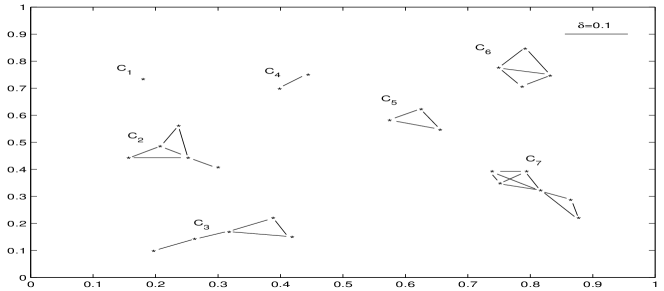
Figure 1: A simplified representation of the invasion percolation algorithm. We show, in a 2D space, some points (i.e. bonds, $B_{i}$) connected by links whose length is less than $\delta$. Each connected group forms a cluster, $C_{i}$.

With this choice we have that the minimal distance between two clusters is greater than $\delta$.

The number of clusters can vary between $N$ disconnected clusters of size $1$ (by size we mean the number of bonds in the cluster) when $\delta=0$, and $1$ large cluster of size $N$ when $\delta=\sqrt{2}$. According to standard percolation-theory [4] a critical percolation threshold $0<\delta_{c}<\sqrt{2}$ is expected: $\delta_{c}$ is the smallest distance for which only $1$ cluster appears.

This technique allows to gain information about the topological structure of the bonds’ space using the distance (1). Other methods, which do not depend on a distance parameter, like $\delta$, are less effective than our invasion-percolation tool.

We found that there are essentially three distinct clusters $C_{1}$,$C_{2}$ and $C_{3}$, up to the critical percolation threshold $\delta_{c}\sim 0.347$:

• is a very small cluster consisting of just a single bond, which is absorbed by the merge of $C_{2}$ and $C_{3}$ at the percolation threshold $\delta_{c}\sim 0.347$ (in the Figure 3 $C_{1}$ is the bond 80).

• is a medium-size very compact cluster. It consists of $29$ bonds which groups together when $\delta\sim 0.087$. This cluster does not change up to $\delta<0.325$, when it finally merges with $C_{3}$.

• is the largest cluster which forms roughly at $\delta\sim 0.157$ and absorbs a variety of micro-clusters up to $\delta<0.305$ as well as $C_{2}$ at $\delta>0.325$.

In Figure 2 we show the diameter of the clusters, $D_{c}(\delta)$ at varying $\delta$. We define

$$D_{c}(\delta)\equiv\max_{i,j\in C_{c}}d(i,j)\,\,.$$ (2)

The diameter gives information about the spread of a cluster. From the Figure 2 one can see the clusters formation of $C_{2}$ and $C_{3}$.

Figure 2: Clusters formation. The top half (b) describes the $C_{3}$ cluster whereas the bottom half (a) refers to $C_{2}$. In each half, the upper continuous line represents the evolution of the clusters’ diameter. Each other line represents the evolution of single bonds (or small cluster) which are absorbed by the main cluster. We have shown only ten bonds for clusters (which are the same as Figure 3). The collapse of two lines implies the merge of the corresponding clusters.

An alternative representation of the cluster structure is offered by the graph in Figure 3 that consists of lines (having the shape of an “upside-down U”) connecting bonds in a hierarchical tree built by means of a linkage algorithm [5]. The height of each U line is the distance between two clusters. In Figure 3, for the sake of clarity, just a subset of bonds is included in the dendrogram (that is the name of this particular graph). Besides the existence of three main classes of bonds, the dendrogram makes easier to locate the “distance” between these groups. We recall that such a distance has a financial meaning since it measures the correlation among bonds and bond classes.

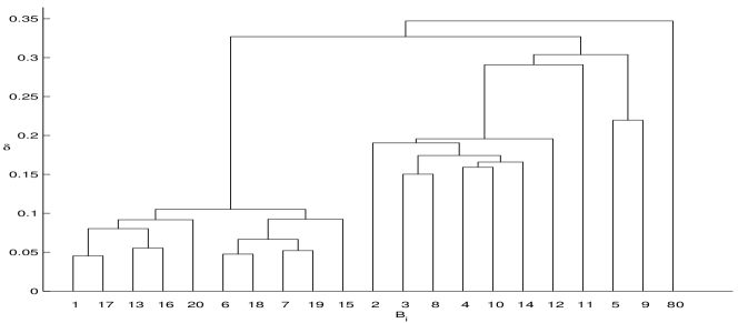
Figure 3: Dendrogram representing the cluster structure of the bonds. Each horizontal line measures at which $\delta$ we have a fusion between two bonds, a bond and a cluster or two clusters.

Taking into account the features of the FI securities which form the three clusters, some additional considerations can be made.

No FI security with maturity greater than 12 years is found in $C_{1}$ and $C_{3}$ whereas the second cluster, $C_{2}$, is composed exclusively by such “long term” bonds. It is worthy to note that for this class of bonds no replicating portfolio can be determined meaning that direct test of the one-price law is not possible. Nevertheless, $C_{2}$ is very compact (the maximum diameter $D$ is equal to 0.2077 ) meaning that the correlation among the corresponding FI securities is very strong.

Usually only large risk-adverse investors (like insurance companies or mutual funds) are interested in long term bonds (whose maturity can be up to thirty-years for US Treasury issues), so a possible explanation is that their expectations (that take into account a number of macroeconomics factors) about the market evolution are so similar that the behavior of long term bonds prices does not reflect any difference in the perceived value of such assets.

Third cluster collects all the other securities, which are the various short and medium term obligations. For many of these assets it is possible to find a replicating portfolio that fulfills the one-price law. However, the profile of the people interested in these assets is much more variegated so the investors may act in many different ways. Such situation generates a minor correlation among the assets, that is, on average, a larger distance. This is reflected in the structure of $C_{3}$ that is wider than $C_{2}$.

So it looks like that, in spite of its clear and unambiguous definition, the correlations imposed by the one-price law are weaker than those produced by “common expectations” of few large investors.

From the theoretical point of view a non perfect correlation among the bonds returns implies that “classical” single factor models for the term structure of interest rate like those by Vasicek [6] or Cox, Ingersoll and Ross [7] can not explain the complex behavior of empirical data.

Besides the correlations among the FI securities, we have analyzed the properties of bond price dynamics. The price fluctuations of a single bond may give an insight into the problem of FI markets efficiency [1]. If price increments are uncorrelated variables, with zero mean value, it is not possible to extract any information about the future evolution of an asset price by looking at its fluctuations in the past (“weak” efficiency).

From Bachelier [8] to nowadays many attempts have been performed to model the statistical properties of financial time series. The distribution function for the returns was considered for a long time a zero mean Gaussian. Mandelbrot proposed, in 1963 [9], a Levy distribution for $r_{t}$. Recently Mantegna and Stanley [10] found that a truncate Levy distribution fits very well the experimental data. Regardless of the specific distribution function, all these models assume that the returns are independent random variables. When the increments $r_{t}$ are, at least, uncorrelated (that is a weaker condition compared to the independence) a model is considered belonging to the the class of “random walks”.

To obtain information about the probability distribution of the price increments we study the moments of

$$r_{t}(\tau)=\sum_{t^{\prime}=1}^{\tau}r_{t+t^{\prime}}=\ln\frac{P_{t+\tau}}{P_{t}}\,\,,$$ (3)

The Structure Function [11] is widely used in fully developed turbulence to study the fluctuations of the velocity field of a fluid. In our case, the study of the moments of $r_{t}(\tau)$ is equivalent to the study of the structure function of the logarithmic price:

$$S_{q}(\tau)\equiv\langle|r_{t}(\tau)|^{q}\rangle_{t}=\langle|\ln P_{t+\tau}-\ln P_{t}|^{q}\rangle_{t}\,\,.$$ (4)

The theory of stable distributions [12] states that, in case of independent variables, the moments behave as $S_{q}(\tau)\sim\tau^{hq}$, where $h$ is the characteristic exponent of the process. For Gaussian increments (actually, in all cases where the central limit theorem applies) $h$ is equal to $1/2$.

We have computed $S_{q}(\tau)$ for bonds belonging to each cluster described above and we found that $S_{q}(\tau)\sim\tau^{\zeta(q)}$ where $\zeta(q)$ is a non linear function. The exponents have been evaluated by means of the Extended-Self-Similarity technique, which consists in log-plotting the generic $p^{th}$ order structure function $S_{p}$ versus $S_{2}$ instead of $\tau$ [13]. One of the advantages of the ESS is that it offers a higher level of statistical confidence since it minimizes finite-size effects.

Figure 4: $\zeta(q)$ versus $q$ for representative bonds belonging to the three main clusters: $C_{1}$ ($\Box$), $C_{2}$ (+) and $C_{3}$ ($\circ$).

The results reported in Figure 4 provide solid evidence of a multi-fractal behavior on top of a random walk, $h=1/2$, for clusters $C_{2}$ and $C_{3}$. All the bonds belonging to the cluster $C_{2}$ show the same scaling exponents (variations are smaller than few part-per-thousand), instead for the cluster $C_{3}$ the scaling behaviour is more variable, but it always shows a non linear $\zeta(q)$.

It is apparent that the bond which is less correlated with others, that is the single bond belonging to $C_{1}$ has a scaling behaviour closer to that expected for a random walk.

The non-linearity of $\zeta(q)$ indicates that the $r_{t}$ are not independent. This means that the random walk hypothesis for the price increments in FI markets does not apply. Similar analyses based on the the structure function have been performed for currency and equity markets [14, 15]. In both cases the signals show a multi-fractal behavior, which definitely brings toward models with non independent price increments.

From a statistical point of view, the multifractality of a signal implies different probability distribution functions of the $r_{t}(\tau)$ at different scales $\tau$. In financial terms this means that price fluctuations of different magnitude behave in a non-uniform way. For instance, the clear concave-shape of $\zeta(q)$ for large $q$ in Figure 4 indicates that large price fluctuations have an anti-persistent behavior (specially for the bonds in $C2$).

Recently, it has been pointed out by [16] that it is possible to get an apparent multifractal behaviour due to strong time correlations of returns. In our data set, however, the most interesting point is that bonds within a cluster behave in a homogeneous way whereas there are remarkable differences between the clusters.

We like to stress that the failure of the random walk hypotheses does not entail that it is easy to develop “strategies” for taking advantage of the correlations present in the bonds’ price increments. At this time, the only evidence is that conventional ARCH (Auto Regressive Conditional Heteroskedasticity) models are incompatible with the scaling properties of price fluctuations.

By now, financial markets analysts have started to accept that the fine structure of the securities markets and frictions in the trading process can generate a certain degree of predictability [17]. However, much work remains to be done because no existing model is able to explain the behavior of price increments across a range of different time scales. Maybe, to reach this goal, it is necessary to model the behavior of the agents, people who buy and sell assets. In [18] the properties of the time series in an artificial stock market have been studied. We expect to perform a similar experiment for the fixed income market.

We thank INA-SGR for providing us with the data used in this work and Dr. Alberto Cybo-Ottone for useful discussions.

References

- [1] E. F. Fama, Efficient capital markets: a review of theory and empirical work, J. Finance 25 (1970) 383–417.
-
[2]
L. Marangio, A. Ramponi and M. Bernaschi
A critical review of techniques for term structure analysis,
submitted to International Journal of Theoretical and Applied Finance - [3] R. N. Mantegna, Hierarchical structure in financial markets, Eur. Phys. J. B 25 (1999) 193–197.
- [4] D. Stauffer and A. Aharony, Introduction to Percolation Theory, (Taylor and Francis, London, 1994)
- [5] P. Griffiths, I. D. Hill and E. Horwood, Applied Statistics Algorithms, (Chichester, 1985).
- [6] O. A. Vasicek, An Equilibrium Characterization of the Term Structure, Journal of Financial Economics 5 (1977), 177–188.
- [7] J. C. Cox, J. E. Ingersoll and S. A. Ross, A Theory of the Term Structure of Interest Rates, Econometrica 53 (1985), 385–408.
- [8] L. Bachelier, Théorie de la spéculation, Ann. Sci École Norm. Sup. 17 (1900) 21–86.
- [9] B. B. Mandelbrot, The variation of certain speculative prices, J. Business 36 (1963) 394–419.
- [10] R. Mantegna and H. E. Stanley, Scaling behavior in the dynamics of an economics index, Nature 376 (1995) 46–49.
- [11] U. Frisch, Turbulence : the legacy of Kolmogorov, (Cambridge University Press, Cambridge U.K., 1995).
- [12] B. V. Gnedenko and A. N. Kolmogorov, Limit Distributions for Sums of Indipendent Random Variables, (Reading, Mass., 1954).
- [13] R. Benzi, S. Ciliberto, R. Tripiccione, F. Massaioli, C. Baudet and S. Succi, Phys. Rev. E 48 R29 (1993).
- [14] R. Baviera, M. Pasquini, M. Serva, D. Vergni and A. Vulpiani, Efficiency in foreign exchange markets, http://xxx.lanl.gov/abs/cond-mat/9901225 (1999).
- [15] M.-E. Brachet, E. Taflin and J.M. Tcheou, Scaling transformation and probability distribution for financial time series, http://xxx.lanl.gov/abs/cond-mat/9905169 (1999).
- [16] J.-P. Bouchaud, M. Potters and M. Meyer, Apparent multifractality in financial time series, http://xxx.lanl.gov/abs/cond-mat/9906347 (1999).
- [17] J. Y. Campbell, A. W. Lo and A. C. MacKinlay, The Econometrics of Financial Markets (Princeton University Press 1997)
- [18] B. LeBaron, W. B. Arthur and R. Palmer, Time Series Properties of an Artificial Stock Market, J. Economic Dynamics and Control 23 (1999), 1487–1516