[

Reactive Hall response

Abstract

The zero temperature Hall constant $R_{H}$, described by reactive (nondissipative) conductivities, is analyzed within linear response theory. It is found that in a certain limit, $R_{H}$ is directly related to the density dependence of the Drude weight implying a simple picture for the change of sign of charge carriers in the vicinity of a Mott-Hubbard transition. This novel formulation is applied to the calculation of $R_{H}$ in quasi-one dimensional and ladder prototype interacting electron systems.

]

It is now well known that in strongly correlated systems the, zero temperature (T=0), reactive part of the conductivity can be used as a criterion of a metallic or insulating ground state[1]. In particular, following the work of Kohn, the imaginary part of the conductivity, $\sigma^{\prime\prime}(\omega\rightarrow 0)=2D/\omega$, characterized by $D$ (now called the “Drude weight” or charge stifness), can be related to the ground state energy density $\epsilon^{0}$ dependence on an applied fictitious flux $\phi$ as $D=(1/2)\partial^{2}\epsilon^{0}/\partial\phi^{2}|_{\phi\rightarrow 0}$.

A similar question is posed by the doping of an insulating state, where it would be interesting to have a simple description of the charge carriers sign as probed in a Hall experiment. For instance, we would like to describe the doping of a Mott-Hubbard insulator; within a semiclassical approach it is expected that the Hall constant $R_{H}\simeq+1/e\delta$, hole-like (positive) near half-filling ($\delta=1-n$, $n$=density), changing to $R_{H}\simeq-1/en$, electron-like at low densities, the turning point depending on the interaction.

Over the recent years, ingenious ways have been proposed[2, 3] for characterizing this sign change and strongly correlated electron systems, as the $t-J$ model have been studied. In particular, following the suggestion to focus at the T=0 Hall constant within linear response theory[5], the $R_{H}$ of a hole in the $t-J$ model was analyzed and a numerical method was proposed for calculating the Hall response in ladder systems[6]. This activity is partly motivated by the physics of high temperature superconductors viewed as doped Mott-Hubbard insulators and related Hall measurements showing a change of the sign of carriers with doping[4].

In this work, we will show that within a certain frequency-$\omega$, wavevector-$q$ limiting procedure, the T=0, $\omega\rightarrow 0$, thus “reactive” Hall constant, is simply related to the density dependence of the Drude weight. Following this point of view, we recover in a straightforward way: (i) the semiclassical expressions for $R_{H}$ at low density and near an insulating state, (ii) a physical picture of the sign change of carriers in the vicinity of a Mott-Hubbard transition and its dependence on interaction strength, (iii) a common expression used to describe the Hall constant in quasi-one dimensional conductors described by a band picture[7], (iv) good accord with $R_{H}$ for ladder systems calculated using the numerical method proposed in [6].

The Hamiltonian  In the following we will consider a generic Hamiltonian for fermions on a lattice, where for simplicity we describe the kinetic energy term by a one band tight binding model; it is straightforward to extend this formulation to a many-band or continuum system. The sites are labeled $l(m)$ along the $x(y)$-direction with periodic boundary conditions in both directions:

$$H = (-t)\sum_{l,m}e^{i\phi^{x}(t)}e^{iA_{m}}c^{\dagger}_{l+1,m}c_{l,m}+h.c.$$ (1)

$$+ (-t^{\prime})\sum_{l,m}e^{i\phi^{y}_{m+1/2}(t)}c^{\dagger}_{l,m+1}c_{l,m}+h.c.$$ (2)

$$+ \hat{U},~{}~{}~{}~{}~{}~{}l=1,...,L_{x};~{}~{}m=1,...,L_{y}.$$ (3)

$c_{l,m}(c^{\dagger}_{l,m})$ is an annihilation (creation) operator at site $(l,m)$ and the spin is neglected as it enters in a trivial way in the formulation. The $\hat{U}$ term can represent a many-particle interaction or a one particle potential. We take the lattice constant so as to consider a unit volume, electric charge $e=1$ and $\hbar=1$. We add a magnetic field along the $z$-direction, modulated by a one component wavevector-$q$ along the $y$-direction, generated by the vector potential $A_{m}$; this allows to take the zero magnetic field limit smoothly[8]:

$$A_{m} = e^{iqm}\frac{iB}{2\sin(q/2)}\simeq e^{iqm}\frac{iB}{q}$$ (4)

$$B_{m+1/2} = -(A_{m+1}-A_{m})=Be^{iq(m+1/2)}$$ (5)

(for convenience, we will present the long wavelength limit, substituting $2\sin(q/2)\rightarrow q$). Electric fields along the $x,y$ directions are generated by time dependent vector potentials:

$$\phi^{x,y}(t) = \frac{E^{x,y}(t)}{iz},~{}~{}\phi^{y}_{m+1/2}(t)=e^{iq(m+1/2)}\phi^{y}(t);$$ (6)

$$E^{x}(t) = E^{x}e^{-izt},~{}~{}E^{y}(t)=iE^{y}e^{-izt};~{}~{}~{}z=\omega+i\eta~{}.$$ (7)

Currents are defined through derivatives of the Hamiltonian expanded to second order in $\phi^{x,y}$:

$$J^{x}=-\frac{\partial H}{\partial\phi^{x}},~{}~{}~{}~{}~{}~{}J^{y}_{q}=-\frac{\partial H}{\partial\phi^{y}}~{},$$ (8)

with the paramagnetic parts:

$$j^{x} = t\sum_{l,m}(ie^{iA_{m}}c^{\dagger}_{l+1,m}c_{l,m}+h.c.)$$ (9)

$$j^{y}_{q} = t^{\prime}\sum_{l,m}e^{iq(m+1/2)}(ic^{\dagger}_{l,m+1}c_{l,m}+h.c.).$$ (10)

The reactive Hall response  From standard linear response theory we obtain:

$$\langle J^{x}\rangle = \sigma_{j^{x}j^{x}}E^{x}(t)+\sigma_{j^{x}j^{y}_{q}}E^{y}(t)$$ (11)

$$\langle J^{y}_{q}\rangle = \sigma_{j^{y}_{q}j^{x}}E^{x}(t)+\sigma_{j^{y}_{q}j^{y}_{q}}E^{y}(t)~{}.$$ (12)

$\langle...\rangle$ are ground state expectation values in the presence of the magnetic field, with the conductivities

$$\sigma_{j^{\alpha}j^{\beta}} = \frac{i}{z}(\langle\frac{\partial^{2}H}{\partial\phi^{\alpha}\partial\phi^{\beta}}\rangle-\chi_{j^{\alpha}j^{\beta}}),$$ (13)

$$\chi_{AB} = i\int^{\infty}_{0}dte^{izt}\langle[A(t),B]\rangle.$$ (14)

Now, in contrast to the usual derivation of the Hall constant expression, we will keep the $q-$dependence explicit by converting the current-current to current-density correlations using the continuity equation:

$$\langle J^{x}\rangle = \sigma_{j^{x}j^{x}}E^{x}(t)+\frac{1}{q}\chi_{j^{x}n_{q}}E^{y}(t)$$ (15)

$$\langle J^{y}_{q}\rangle = -\frac{1}{q}\chi_{n_{q}j^{x}}E^{x}(t)+(\frac{z}{q})^{2}\chi_{n_{q}n_{q}}\frac{i}{z}E^{y}(t)~{},$$ (16)

with $n_{q}=\sum_{l,m}(-ie^{iqm})c^{\dagger}_{l,m}c_{l,m}$.

At T=0, the response is non-dissipative so we will study the reactive (out-of phase) induced currents. Furthermore, at this point we will consider the “screening” (or slow) response in the $y-$direction, by taking the $(q,\omega)$ limits in the order $\omega\rightarrow 0$ first and $q\rightarrow 0$ last; in the usual “transport” (or fast) response the limits are in the opposite order[9]. As we will discuss below, this approach leads to a simple physical picture for the Hall constant and it might be argued that at least for certain cases, for example for a system of finite size in the $y-$direction, it is indeed the right one. The expressions (16) for the currents become:

$$\langle J^{x}\rangle_{0} = \sigma_{j^{x}j^{x}}^{\prime\prime}(\omega\rightarrow 0))(iE^{x}(t))$$ (17)

$$+ \frac{1}{q}\chi_{j^{x}n_{q}}^{\prime}(\omega=0)E^{y}(t)$$ (18)

$$\langle J^{y}_{q}\rangle_{0} = -\frac{1}{q}\chi_{n_{q}j^{x}}^{\prime}(\omega=0)E^{x}(t)$$ (19)

$$+ (\frac{\omega}{q})^{2}\frac{1}{\omega}\chi_{n_{q}n_{q}}^{\prime}(\omega=0)(iE^{y}(t))~{},$$ (20)

where the subscript zero denotes the leading order in $\omega$ response,

$$\chi_{AB}^{\prime}(\omega=0)=\sum_{n>0}\frac{\langle 0|A|n\rangle\langle n|B|0\rangle+h.c.}{E_{n}-E_{0}},$$ (21)

and $|n\rangle(E_{n})$ are eigenstates (eigenvalues) of the Hamiltonian in the presence of the magnetic field.

Now, following Kohn’s observation[1], we can identify the different terms as derivatives of the ground state energy density $\epsilon^{0}$ of a fictitious Hamiltonian depending on static $\phi^{x},\mu_{q}$ fields:

$$H = (-t)\sum_{l,m}(e^{i\phi^{x}}e^{iA_{m}}c^{\dagger}_{l+1,m}c_{l,m}+h.c.)$$ (22)

$$+ (-t^{\prime})\sum_{l,m}(c^{\dagger}_{l,m+1}c_{l,m}+h.c.)+\mu_{q}n_{q}+\hat{U}.$$ (23)

For $H(\lambda,\mu)$, using the following identity,

$$\epsilon^{0}_{\mu\lambda}=\frac{\partial^{2}\epsilon^{0}}{\partial\mu\partial\lambda} = \langle 0|\frac{\partial^{2}H}{\partial\mu\partial\lambda}|0\rangle$$ (24)

$$- \sum_{m>0}\frac{\langle 0|\frac{\partial H}{\partial\mu}|m\rangle\langle m|\frac{\partial H}{\partial\lambda}|0\rangle+h.c.}{E_{m}-E_{0}}~{},$$ (25)

we can rewrite the currents as:

$$\langle J^{x}\rangle_{0} = \frac{\epsilon^{0}_{\phi^{x}\phi^{x}}}{\omega}(iE^{x}(t))+(\frac{-1}{q})\epsilon^{0}_{\phi^{x}\mu_{q}}E^{y}(t)$$ (26)

$$\langle J^{y}_{q}\rangle_{0} = \frac{1}{q}\epsilon^{0}_{\mu_{q}\phi^{x}}E^{x}(t)-\frac{\omega}{q^{2}}\epsilon^{0}_{\mu_{q}\mu_{q}}(iE^{y}(t)).$$ (27)

Finally, setting $\langle J^{y}_{q}\rangle_{0}=0$ we determine the “reactive” Hall constant:

$$R_{H}\equiv-\frac{1}{B}\frac{E^{y}}{\langle J^{x}\rangle_{0}}=(-\frac{q}{B})\frac{\epsilon^{0}_{\mu_{q}\phi^{x}}}{\epsilon^{0}_{\phi^{x}\phi^{x}}\epsilon^{0}_{\mu_{q}\mu_{q}}+\epsilon^{0}_{\mu_{q}\phi^{x}}\epsilon^{0}_{\phi^{x}\mu_{q}}}~{}.$$ (28)

Neglecting the cross-terms $\epsilon^{0}_{\mu_{q}\phi^{x}}\epsilon^{0}_{\phi^{x}\mu_{q}}$ and Taylor expanding the numerator in $B$, we can rewrite $R_{H}$ as:

$$R_{H}=q\frac{\frac{\partial^{3}\epsilon^{0}}{\partial B\partial\mu_{q}\partial\phi^{x}}}{\epsilon^{0}_{\phi^{x}\phi^{x}}\epsilon^{0}_{\mu_{q}\mu_{q}}}=q\frac{\frac{\partial}{\partial\mu_{q}}(\frac{\partial^{2}\epsilon^{0}}{\partial B\partial\phi^{x}})}{\epsilon^{0}_{\phi^{x}\phi^{x}}\epsilon^{0}_{\mu_{q}\mu_{q}}}~{}.$$ (29)

Using (25) we find the final expression:

$$R_{H}=-\frac{\frac{\partial D_{q}}{\partial\mu_{q}}}{D\kappa_{q}}$$ (30)

where,

$$D_{q} = \frac{1}{2}[\langle 0|-T^{x}_{q}|0\rangle$$ (31)

$$- \sum_{m}\frac{\langle 0|j^{x}|m\rangle\langle m|j^{x}_{q}|0\rangle+h.c.}{\epsilon_{m}-\epsilon_{0}}],$$ (32)

$$j^{x}_{q} = (-t)\sum_{l,m}(-ie^{iqm})(ic^{\dagger}_{l+1,m}c_{l,m}+h.c.),$$ (33)

$$T^{x}_{q} = (-t)\sum_{l,m}(-ie^{iqm})(c^{\dagger}_{l+1,m}c_{l,m}+h.c.).$$ (34)

$D=\frac{1}{2}\epsilon^{0}_{\phi^{x}\phi^{x}}$, the Drude weight, is identical to $D_{q}$ by the replacement of $j^{x}_{q}$ ($T^{x}_{q}$) by $j^{x}$ ($T^{x}$). $\kappa_{q}=\epsilon^{0}_{\mu_{q}\mu_{q}}=\partial n_{q}/\partial\mu_{q}$ is the compressibility corresponding to the density modulation $n_{q}$. Notice that the spatial dependence of $j^{x}_{q}$ and $n_{q}$ is the same as that of $A_{m}$.

Taking the $q\rightarrow 0$ limit, we obtain a particularly simple expression for $R_{H}$:

$$R_{H}=-\frac{1}{D}\frac{\partial D}{\partial n}.$$ (35)

A handwaving argument leading to expression (35) for $t^{\prime}\to 0$ is as follows: $A_{m}$ corresponds to a twist of boundary conditions on chain$-m$, inducing an extra current on each chain proportional to $D$ (besides the uniform one induced by the flux $\phi^{x}$); minimization of the energy at fixed $x-$current gives rise to an $m-$dependent charge density. This induced charge density can then be canceled by the “Hall potential” $\mu_{q}$[6]. Note that a similar idea, analyzing the Hall constant in terms of independent channels (edge states), exists in the literature of the Quantum Hall effect[10].

This expression is appealing as it gives a direct, intuitive understanding for the change of sign of charge carriers in the vicinity of a metal-insulator transition. First, at low densities, $D\propto n$ giving $R_{H}\simeq-1/n$; close to a Mott insulator $D\propto\delta=1-n$, implying $R_{H}\simeq+1/\delta$. Furthermore, we obtain a change of sign in the vicinity of a Mott transition at a density which depends on the interaction strength and is given by the position of the maximum of $D$. Second, for independent electrons, where $D$ is proportional to the kinetic energy, by taking the limit $t^{\prime}\rightarrow 0$ and calculating $D$ as a sum of $D$’s for individual $x-$chains, we obtain from (35):

$$D=\frac{2t}{\pi}\sin(\frac{\pi n}{2}),~{}~{}~{}R_{H}=-\frac{\pi}{2}\frac{1}{\tan(\frac{\pi n}{2})},$$ (36)

an expression used for the Hall constant of quasi one-dimensional compounds[7]. Considering that the $t^{\prime}\rightarrow 0$ limit might by subtle, it is of particular theoretical and experimental interest whether the Hall constant of quasi-one dimensional correlated systems [11] is indeed given by the expression and thus related to the Drude weight of the individual chains. The same applies for the transverse Hall effect of weakly coupled planes.

Examples  In this section we present a generic picture for the behavior of the Hall constant for models of strongly correlated fermions showing a Mott-Hubbard metal-insulator transition. This picture emerges, on the one hand, by an exact calculation of $R_{H}$ for ladder systems using the numerical method of ref.[6] and on the other hand, from the expression (35) assuming nearly decoupled chains ($t^{\prime}\rightarrow 0$) and calculating $D(n)$ for each chain analytically using the Bethe ansatz method[12, 13]. It is clear that this analytical approach refers to either ladder (with $t^{\prime}\rightarrow 0$) or quasi one-dimensional models.

Three prototype models will be discussed: the Hubbard model, as the most experimentally relevant, the spinless fermions model (“t-V”) showing both a metallic and an insulating phase depending on interaction strength and the supersymmetric $t-J$ model.

(i) The Hubbard model is given by the Hamiltonian:

$$H =(-t)\sum_{l,m}(c^{\dagger}_{l+1,m,\sigma}c_{l,m,\sigma}+h.c.)$$ (37)

$$+ (-t^{\prime})\sum_{l,m}(c^{\dagger}_{l,m+1,\sigma}c_{l,m,\sigma}+h.c.)+U\sum_{l,m}n_{l,m,\uparrow}n_{l,m,\downarrow}~{}.$$ (38)

$c_{l,m,\sigma}(c^{\dagger}_{l,m,\sigma})$ is an annihilation (creation) operator at site $(l,m)$ of a fermion with spin $\sigma=\uparrow,\downarrow$. $R_{H}$ extracted from a Bethe ansatz calculation of $D(n)$ for the one dimensional Hubbard model[13] is shown in Fig. 1.

FIG. 1.: $R_{H}$ for the Hubbard model from expression (35) for $t^{\prime}\rightarrow 0$.

This behavior is characteristic of correlated systems undergoing a metal-insulator transition at half-filling: at low densities $R_{H}\simeq-1/n$, while near half-filling $R_{H}\simeq+1/\delta$, the position of change of sign of the carriers depending on the details of the interaction.

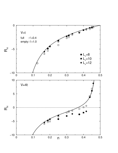
(ii) The t-V model on a ladder is given by:

$$H = (-t)\sum_{l,m}(c^{\dagger}_{l+1,m}c_{l,m}+h.c.)$$ (39)

$$+ (-t^{\prime})\sum_{l}(c^{\dagger}_{l,1}c_{l,2}+h.c.)+V\sum_{l,m}n_{l,m}n_{l+1,m}.$$ (40)

Here and in the following $l=1,...,L_{x},m=1,2$. For a single chain, this model describes a metallic phase at all densities for $V<2t$, while for $V>2t$ it is an insulator at half-filling. In Fig. 2 we show $R_{H}$ calculated numerically on finite systems for two values of $t^{\prime}$ and analytically from (35) in the $t^{\prime}\rightarrow 0$ limit. The numerical evaluation being especially sensitive to finite size effects for $t^{\prime}\rightarrow 0$, we study relatively large values of $t^{\prime}$.

Results for $R_{H}$ clearly show the difference between the metallic regime $V=t$, where at half-filling ($n=0.5$) we get $R_{H}=0$, while in the insulating regime $V=4t$, we are dealing with $R_{H}(n\to 0.5)\to\infty$.

FIG. 2.: $R_{H}$ for the $t-V$ ladder from expression (35) for $t^{\prime}\rightarrow 0$ (continuous line) and from a numerical evaluation (symbols). $V=t(4t)$, metallic (insulating) phase at $n=0.5$.

(iii) The t-J model on a ladder is given by the Hamiltonian:

$$H = (-t)\sum_{l,m}(c^{\dagger}_{l+1,m,\sigma}c_{l,m,\sigma}+h.c.)$$ (41)

$$+ (-t^{\prime})\sum_{l}(c^{\dagger}_{l,1,\sigma}c_{l,2,\sigma}+h.c.)$$ (42)

$$+ J\sum_{l,m}(\vec{S}_{l,m}\vec{S}_{l+1,m}-\frac{1}{4}n_{l,m}n_{l+1,m})~{}.$$ (43)

$\vec{S}_{lm}$ is the spin operator at site $(l,m)$ and the double occupancy on a site is forbidden.

FIG. 3.: $R_{H}$ for the $t-J$ ladder from expression (35) for $t^{\prime}\rightarrow 0$ (continuous line) and from a numerical evaluation (symbols).

In Fig. 3 we show again $R_{H}$ calculated analytically for the “supersymmetric” model, $J=2t$, and by numerical evaluation for $t^{\prime}=0.5t$ and different size systems.

The above three examples show a remarkable agreement between the numerical evaluation of $R_{H}$ on finite size systems using the method of ref.[6] (at finite $t^{\prime}$) and the analytical calculation using (35) for $t^{\prime}\rightarrow 0$, indicating a relative insensitivity on the transverse coupling $t^{\prime}$ for ladders. These results confirm the intuitive picture for the behavior of the Hall constant in the vicinity of a metal-insulator transition and present an intriguing link between the Hall constant and the Drude weight. It is possible that $R_{H}$ is dominated at low temperatures by correlations and not the relaxation mechanism so this formulation could have more general validity.

In conclusion, the emerging simple physical picture raises the question of the relation of this novel formulation to the traditional semiclassical approach to the Hall constant, its range of validity, the role of relaxation in the description of the Hall effect and of the perspectives for an extension at finite temperatures.

Part of this work was done during visits of (P.P.) and (M.L.) at IRRMA as academic guests of EPFL. X.Z. and F.N. acknowledge support by the Swiss National Foundation grant No. 20-49486.96, the EPFL, the Univ. of Fribourg and the Univ. of Neuchâtel.

REFERENCES

• [1] W. Kohn, Phys. Rev. 133, A171 (1964).
• [2] H. E. Castillo and C. A. Balseiro, Phys. Rev. Lett. 68, 121 (1992).
• [3] A.G. Rojo, G. Kotliar and G.S. Canright, Phys. Rev. B57, 9140 (1993).
• [4] For a review see e.g. N. P. Ong, in Physical Properties of High Temperature Superconductors, ed. by D. M. Ginsberg (World Scientific, Singapore, 1990), Vol. 2.
• [5] P. Prelovšek, Phys. Rev. B 55, 9219 (1997).
• [6] P. Prelovšek, M. Long, T. Markež and X. Zotos, Phys. Rev. Lett. 83, 2785 (1999).
• [7] J.R. Cooper et al., J. Phys. (Paris) 38, 1097 (1977); K. Maki and A. Virosztek, Phys. Rev. B41, 557 (1990).
• [8] H. Fukuyama, H. Ebisawa, and Y. Wada, Prog. Teor. Phys. 42, 495 (1969)
• [9] J.M. Luttinger, Phys. Rev. 135, A1505 (1964).
• [10] B.I. Halperin, Phys. Rev. B25, 2185 (1982).
• [11] or of the stripe phase in high Tc compounds; T. Noda, H. Eisaki and S. Uchida, Science 286, 265 (1999).
• [12] F.D.M. Haldane, Phys. Lett. 81A, 153 (1981).
• [13] N. Kawakami and S-K. Yang, Phys. Rev. B44, 7844 (1991).