Rouse Chains with Excluded Volume Interactions: Linear Viscoelasticity

Abstract

Linear viscoelastic properties for a dilute polymer solution are predicted by modeling the solution as a suspension of non-interacting bead-spring chains. The present model, unlike the Rouse model, can describe the solution’s rheological behavior even when the solvent quality is good, since excluded volume effects are explicitly taken into account through a narrow Gaussian repulsive potential between pairs of beads in a bead-spring chain. The use of the narrow Gaussian potential, which tends to the more commonly used $\delta$-function repulsive potential in the limit of a width parameter $d$ going to zero, enables the performance of Brownian dynamics simulations. The simulations results, which describe the exact behavior of the model, indicate that for chains of arbitrary but finite length, a $\delta$-function potential leads to equilibrium and zero shear rate properties which are identical to the predictions of the Rouse model. On the other hand, a non-zero value of $d$ gives rise to a prediction of swelling at equilibrium, and an increase in zero shear rate properties relative to their Rouse model values. The use of a $\delta$-function potential appears to be justified in the limit of infinite chain length. The exact simulation results are compared with those obtained with an approximate solution which is based on the assumption that the non-equilibrium configurational distribution function is Gaussian. The Gaussian approximation is shown to be exact to first order in the strength of excluded volume interaction, and is found to be accurate above a threshold value of $d$, for given values of chain length and strength of excluded volume interaction.

1 Introduction

The simplest model, within the context of Polymer Kinetic Theory, to describe the rheological behavior of dilute polymer solutions is the Rouse model [1]. The Rouse model represents the macromolecule by a linear chain of identical beads connected by Hookean springs, and assumes that the solvent influences the motion of the beads by exerting a drag force and a Brownian force. While the Rouse model is able to explain the existence of viscoelasticity in polymer solutions by predicting a constant non-zero first normal stress difference in simple shear flow, it cannot predict several other features of dilute solution behavior, such as the existence of a nonzero second normal stress difference, the existence of shear rate dependent viscometric functions, or the correct molecular weight dependence of material functions. Over the past decade, considerable progress has been made by incorporating the effect of fluctuating hydrodynamic interaction into the Rouse model [2, 3, 4, 5, 6]. These models are able to predict the molecular weight dependence of the material functions accurately. They also predict a nonzero second normal stress difference, and shear rate dependent viscometric functions. However, since they neglect the existence of excluded volume interactions among parts of the polymer chain, they are strictly applicable only to theta solutions.

Recently, Prakash and Öttinger [7] examined the influence of excluded volume effects on the rheological behavior of dilute polymer solutions by representing the polymer molecule with a Hookean dumbbell model, and using a narrow Gaussian repulsive potential to describe the excluded volume interactions between the beads of the dumbbell. The narrow Gaussian potential tends to a $\delta$-function potential in the limit of a parameter, that describes the width of the potential, going to zero. It can therefore be used to evaluate results obtained with the singular $\delta$-function potential. It was shown by them that the use of a $\delta$-function potential between the beads, which is commonly used in static theories for polymer solutions [8, 9, 10], leads to no change in the equilibrium or dynamic properties of the dumbbell when compared to the case where no excluded volume interactions are taken into account. They also found that assuming that the non-equilibrium configurational distribution function is a Gaussian leads to accurate predictions of viscometric functions in a certain range of parameter values. These results suggest that it would be worthwhile examining longer bead-spring chains. Firstly, it is interesting to see if the problem with the $\delta$-function potential can be resolved when there are more beads in the bead-spring chain. Secondly, it is important to find out if the Gaussian approximation is accurate even for longer chains. The purpose of this paper is to attempt to answer these questions, in the linear viscoelastic limit, by extending the methodology developed in the earlier paper to the case of bead-spring chains. The same issues, in the context of steady shear flows at finite shear rates, will be addressed in a subsequent paper.

As in the dumbbell paper, we confine our attention to excluded volume interactions alone, and neglect the presence of hydrodynamic interactions. This clearly implies—since it is essential to include hydrodynamic interaction effects for a proper description of the dynamic behavior of dilute solutions—that the results of the present paper are not yet directly comparable with experiments. They represent a preliminary step in that direction. It is felt that the inclusion of hydrodynamic interaction would make the theory significantly more complex before the role of excluded volume interactions is properly understood. The aim of this work is to develop and carefully evaluate the Gaussian approximation for excluded volume interactions. The Gaussian approximation has already been shown to be excellent for the treatment of hydrodynamic interaction effects [4]. If it also proves to be accurate for the treatment of excluded volume effects, then it would be extremely useful for describing the combined effects of hydrodynamic interaction and excluded volume. It should be noted that, in principle, the development of such an approximation does not pose any fundamental problems.

This paper is organized as follows. In the next section, the basic equations governing the dynamics of Rouse chains with excluded volume interactions are discussed. A retarded motion expansion for the stress tensor is derived in section 3, and exact expressions for the zero shear rate viscometric functions in simple shear flow are obtained. The implications of these results for a $\delta$-function excluded volume potential are then discussed. In section 4, the Brownian dynamics simulation algorithm used in this work is described. Section 5 is devoted to the development of the Gaussian approximation for the configurational distribution function. Exact expressions for linear viscoelastic properties are derived through a codeformational memory-integral expansion. In section 6, a first order perturbation expansion in the strength of the excluded volume interaction is carried out. This proves to be very helpful in understanding the nature of the Gaussian approximation. The results of the various exact and approximate treatments are compared and discussed in section 7, and the main conclusions of the paper are summarized in section 8.

2 Basic Equations

The instantaneous configuration of a linear bead-spring chain, which consists of $N$ beads connected together by $(N-1)$ Hookean springs, is specified by the bead position vectors ${{{\mbox{\boldmath$r$}}}}_{\nu},\,\nu=1,2,\ldots,N,$ in a laboratory-fixed coordinate system. The Newtonian solvent, in which the chain is suspended, is assumed to have a homogeneous velocity field—that is, at position $r$ and time $t$, the velocity is given by ${{\mbox{\boldmath$v$}}}({{\mbox{\boldmath$r$}}},t)={{\mbox{\boldmath$v$}}}_{0}+{\mbox{\boldmath$\kappa$}}(t)\cdot{{{\mbox{\boldmath$r$}}}}$, where ${{\mbox{\boldmath$v$}}}_{0}$ is a constant vector and ${\mbox{\boldmath$\kappa$}}(t)$ is a traceless tensor.

The microscopic picture of the intra-molecular forces within the bead-spring chain is one in which the presence of excluded volume interactions between the beads causes the chain to swell, while on the other hand, the entropic retractive force of the springs draws the beads together and opposes the excluded volume force. This is modeled by writing the potential energy $\phi$ of the bead-spring chain as a sum of the potential energy of the springs $S$, and the potential energy due to excluded volume interactions $E$. The potential energy $S$ is the sum of the potential energies of all the springs in the chain, and is given by,

$$S={1\over 2}\,H\,\sum_{i=1}^{N-1}\,{{{\mbox{\boldmath$Q$}}}}_{i}\cdot{{{\mbox{\boldmath$Q$}}}}_{i}$$ (1)

where, $H$ is the spring constant, and ${{{\mbox{\boldmath$Q$}}}}_{i}={{{\mbox{\boldmath$r$}}}}_{i+1}-{{{\mbox{\boldmath$r$}}}}_{i}$, is the bead connector vector between the beads $i$ and $i+1$. The excluded volume potential energy $E$ is found by summing the interaction energy over all pairs of beads $\mu$ and $\nu$,

$$E={1\over 2}\sum_{\mu,\nu=1\atop\mu\neq\nu}^{N}\,E\left({{{\mbox{\boldmath$r$}}}}_{\nu}-{{{\mbox{\boldmath$r$}}}}_{\mu}\right)$$ (2)

where, $E\left({{{\mbox{\boldmath$r$}}}}_{\nu}-{{{\mbox{\boldmath$r$}}}}_{\mu}\right)$ is a short-range function. It is usually assumed to be a $\delta$-function potential in static theories for polymer solutions,

$$E\left({{{\mbox{\boldmath$r$}}}}_{\nu}-{{{\mbox{\boldmath$r$}}}}_{\mu}\right)=v\,k_{\rm B}T\,\delta\left({{{\mbox{\boldmath$r$}}}}_{\nu}-{{{\mbox{\boldmath$r$}}}}_{\mu}\right)$$ (3)

where, $v$ is the excluded volume parameter (with dimensions of volume), $k_{\rm B}$ is Boltzmann’s constant, and $T$ is the absolute temperature. In this work, we regularise the $\delta$-function potential, and assume that $E\left({{{\mbox{\boldmath$r$}}}}_{\nu}-{{{\mbox{\boldmath$r$}}}}_{\mu}\right)$ is given by a narrow Gaussian potential,

$$E\left({{{\mbox{\boldmath$r$}}}}_{\nu}-{{{\mbox{\boldmath$r$}}}}_{\mu}\right)={v\,k_{\rm B}T\over[2\pi{\tilde{d}}^{2}]^{3\over 2}}\,\exp\left(-{1\over 2}{{{\mbox{\boldmath$r$}}}_{\nu\mu}^{2}\over{\tilde{d}}^{2}}\right)$$ (4)

where, ${\tilde{d}}$ is a parameter that describes the width of the potential (it represents, in some sense, the extent of excluded volume interactions), and ${{\mbox{\boldmath$r$}}}_{\nu\mu}={{\mbox{\boldmath$r$}}}_{\nu}-{{\mbox{\boldmath$r$}}}_{\mu}$, is the vector between beads $\mu$ and $\nu$. In the limit ${\tilde{d}}$ tending to zero, the narrow Gaussian potential becomes a $\delta$-function potential.

The intra-molecular force on a bead $\nu$, ${{{\mbox{\boldmath$F$}}}}_{\nu}^{(\phi)}=-({\partial\phi/\partial{{{\mbox{\boldmath$r$}}}}_{\nu}})$, can consequently be written as, ${{{\mbox{\boldmath$F$}}}}_{\nu}^{(\phi)}={{{\mbox{\boldmath$F$}}}}_{\nu}^{(S)}+{{{\mbox{\boldmath$F$}}}}_{\nu}^{(E)}$, where,

$${{{\mbox{\boldmath$F$}}}}_{\nu}^{(S)} = -{\partial S\over\partial{{{\mbox{\boldmath$r$}}}}_{\nu}}=-H\sum_{k=1}^{N-1}{\overline{B}}_{k\nu}\,{{\mbox{\boldmath$Q$}}}_{k}$$ (5)

$${{{\mbox{\boldmath$F$}}}}_{\nu}^{(E)} = -{\partial E\over\partial{{{\mbox{\boldmath$r$}}}}_{\nu}}=-\sum_{\mu=1\atop\mu\neq\nu}^{N}\,{\partial\over\partial{{\mbox{\boldmath$r$}}}_{\nu}}\,E\left({{{\mbox{\boldmath$r$}}}}_{\nu}-{{{\mbox{\boldmath$r$}}}}_{\mu}\right)$$ (6)

In eq 5, ${\overline{B}}_{k\nu}$ is an $(N-1)\times N$ matrix defined by, ${\overline{B}_{k\nu}}=\delta_{k+1,\;\nu}-\delta_{k\nu}$, with $\delta_{k\nu}$ denoting the Kronecker delta.

For homogeneous flows, the internal configurations of the bead-spring chain are expected to be independent of the location of the centre of mass. Consequently, it is assumed that the configurational distribution function $\psi$ depends only on the $(N-1)$ bead connector vectors ${{\mbox{\boldmath$Q$}}}_{k}$. The diffusion equation that governs $\psi\,({{{\mbox{\boldmath$Q$}}}}_{1},\ldots,{{{\mbox{\boldmath$Q$}}}}_{N-1},t)$, for a system with an intra-molecular potential energy $\phi$ as described above, can then be shown to be given by,

$${\partial\,\psi\over\partial t}= - \sum_{j=1}^{N-1}\,{\partial\over\partial{{{\mbox{\boldmath$Q$}}}}_{j}}\cdot\biggl{(}{\mbox{\boldmath$\kappa$}}\cdot{{{\mbox{\boldmath$Q$}}}}_{j}-{H\over\zeta}\,\sum_{k=1}^{N-1}\,A_{jk}\,{{{\mbox{\boldmath$Q$}}}}_{k}+{1\over\zeta}\,\sum_{\nu=1}^{N}\,{\overline{B}}_{j\nu}{{\mbox{\boldmath$F$}}}_{\nu}^{(E)}\,\biggr{)}\,\psi$$ (7)

$$+ {k_{\rm B}T\over\zeta}\,\sum_{j,\,k=1}^{N-1}\,A_{jk}\;{\partial\over\partial{{{\mbox{\boldmath$Q$}}}}_{j}}\cdot{\partial\psi\over\partial{{{\mbox{\boldmath$Q$}}}}_{k}}$$

where, $\zeta$ is the bead friction coefficient (which, for spherical beads with radius $a$, in a solvent with viscosity $\eta_{s}$, is given by the Stokes expression: $\zeta=6\pi\eta_{s}a$), and $A_{jk}$ is the Rouse matrix,

$$A_{jk}=\sum_{\nu=1}^{N}\,{\overline{B}}_{j\nu}{\overline{B}}_{k\nu}=\cases{2&for $|{j-k}|=0$,\cr\vskip 3.0pt\cr-1&for $|{j-k}|=1$,\cr\vskip 3.0pt\cr 0&otherwise\cr}$$ (8)

The time evolution of the average of any arbitrary quantity, carried out with the configurational distribution function $\psi$, can be obtained from the diffusion equation. In particular, by multiplying eq 7 by ${{{\mbox{\boldmath$Q$}}}}_{j}{{{\mbox{\boldmath$Q$}}}}_{k}$, and integrating over all configurations, the following time evolution equation for the second moments of the bead connector vectors is obtained,

$${d\over dt}\,{\bigl{\langle}}{{{\mbox{\boldmath$Q$}}}}_{j}{{{\mbox{\boldmath$Q$}}}}_{k}{\bigr{\rangle}} = {\mbox{\boldmath$\kappa$}}\cdot{\bigl{\langle}}{{{\mbox{\boldmath$Q$}}}}_{j}{{{\mbox{\boldmath$Q$}}}}_{k}{\bigr{\rangle}}+{\bigl{\langle}}{{{\mbox{\boldmath$Q$}}}}_{j}{{{\mbox{\boldmath$Q$}}}}_{k}{\bigr{\rangle}}\cdot{\mbox{\boldmath$\kappa$}}^{T}+{2k_{\rm B}T\over\zeta}\,A_{jk}\,{{\mbox{\boldmath$1$}}}$$ (9)

$$- {H\over\zeta}\,\sum_{m=1}^{N-1}\,\left\{\,{\bigl{\langle}}{{{\mbox{\boldmath$Q$}}}}_{j}{{\mbox{\boldmath$Q$}}}_{m}{\bigr{\rangle}}\,A_{mk}+A_{jm}\,{\bigl{\langle}}{{{\mbox{\boldmath$Q$}}}}_{m}{{\mbox{\boldmath$Q$}}}_{k}{\bigr{\rangle}}\,\right\}+{{\mbox{\boldmath$Y$}}}_{jk}$$

where, $1$ is the unit tensor, and,

$${{\mbox{\boldmath$Y$}}}_{jk}={1\over\zeta}\,\sum_{\mu=1}^{N}\,\left\{\,{\bigl{\langle}}{{{\mbox{\boldmath$Q$}}}}_{j}{{{\mbox{\boldmath$F$}}}}_{\mu}^{(E)}{\bigr{\rangle}}\,{\overline{B}}_{k\mu}+{\overline{B}}_{j\mu}\,{\bigl{\langle}}{{{\mbox{\boldmath$F$}}}}_{\mu}^{(E)}{{\mbox{\boldmath$Q$}}}_{k}{\bigr{\rangle}}\,\right\}$$ (10)

The term ${{\mbox{\boldmath$Y$}}}_{jk}$, which arises due to the presence of excluded volume interactions, does not appear in the second moment equation for the Rouse model. Due to this term, which in general involves higher order moments, eq 9, is not a closed equation for ${\bigl{\langle}}{{{\mbox{\boldmath$Q$}}}}_{j}{{{\mbox{\boldmath$Q$}}}}_{k}{\bigr{\rangle}}$. As will be discussed in greater detail in the section on the Gaussian approximation, finding an approximate solution for the present model involves making eq 9 a closed equation for the second moments.

The polymer contribution to the stress tensor—for models with arbitrary intra-molecular potential forces but no internal constraints—is given by the Kramers expression [11],

$${{\mbox{\boldmath$\tau$}}}^{p}=-n_{\rm p}H\,\sum_{k=1}^{N-1}\,{\bigl{\langle}}{{{\mbox{\boldmath$Q$}}}}_{k}{{\mbox{\boldmath$Q$}}}_{k}{\bigr{\rangle}}+{{\mbox{\boldmath$Z$}}}+(N-1)\,n_{\rm p}k_{\rm B}T\,{{\mbox{\boldmath$1$}}}$$ (11)

where,

$${{\mbox{\boldmath$Z$}}}=n_{\rm p}\,\sum_{\nu=1}^{N}\sum_{k=1}^{N-1}\,B_{\nu k}\,{\bigl{\langle}}{{\mbox{\boldmath$Q$}}}_{k}{{{\mbox{\boldmath$F$}}}}_{\nu}^{(E)}{\bigr{\rangle}}$$ (12)

Here, $n_{\rm p}$ is the number density of polymers, and $B_{\nu k}$ is a $N\times(N-1)$ matrix defined by, $B_{\nu k}=k/N-\Theta\,(k-\nu)$, with $\Theta\,(k-\nu)$ denoting a Heaviside step function.

It is clear from eq 11 that there are two reasons why the presence of excluded volume interactions leads to a stress tensor that is different from that obtained in the Rouse model. Firstly, there is an additional term represented by $Z$ which is the direct influence of excluded volume effects. Secondly, there is an indirect influence due to a change in the contribution of the term $\sum_{k=1}^{N-1}\,{\bigl{\langle}}{{{\mbox{\boldmath$Q$}}}}_{k}{{{\mbox{\boldmath$Q$}}}}_{k}{\bigr{\rangle}}$, relative to its contribution in the Rouse case. For a $\delta$-function excluded volume potential, it can be shown that the direct contribution to the stress tensor is isotropic [8]. On the other hand, for the narrow Gaussian potential, $Z$ is not isotropic unless $\tilde{d}$ is equal to zero. It is therefore important to use the complete form of the Kramers expression, eq 11, when carrying out simulations with an excluded volume potential that is not a $\delta$-function potential.

All the rheological properties of interest can be obtained once the stress tensor in eq 11 is evaluated. In the next section, a retarded motion expansion for the stress tensor is derived.

3 Retarded Motion Expansion

A retarded motion expansion for the stress tensor can be obtained by extending the derivation carried out previously for the dumbbell model [7] to the case of bead-spring chains. The dumbbell model derivation was, in turn, an adaptation of a similar development for the FENE dumbbell model [11]. The argument in all these cases rests basically on seeking a solution of the diffusion equation, eq 7, of the following form,

$$\psi({{{\mbox{\boldmath$Q$}}}}_{1},\ldots,{{{\mbox{\boldmath$Q$}}}}_{N-1},t)=\psi_{\rm eq}({{{\mbox{\boldmath$Q$}}}}_{1},\ldots,{{{\mbox{\boldmath$Q$}}}}_{N-1})\,\phi_{\rm fl}\,({{{\mbox{\boldmath$Q$}}}}_{1},\ldots,{{{\mbox{\boldmath$Q$}}}}_{N-1},t)$$ (13)

where, $\psi_{\rm eq}$ is the equilibrium distribution function given by,

$$\psi_{\rm eq}({{{\mbox{\boldmath$Q$}}}}_{1},\ldots,{{{\mbox{\boldmath$Q$}}}}_{N-1})={\cal N_{\rm eq}}\,e^{-{\phi/k_{\rm B}T}}$$ (14)

with ${\cal N_{\rm eq}}$ denoting the normalization constant, and $\phi_{\rm fl}$ is the correction to $\psi_{\rm eq}$ due to flow—appropriately termed the flow contribution.

The governing partial differential equation for $\phi_{\rm fl}\,({{{\mbox{\boldmath$Q$}}}}_{1},\ldots,{{{\mbox{\boldmath$Q$}}}}_{N-1},t)$ can be obtained by substituting eq 13 into the diffusion equation, eq 7. It turns out that, regardless of the form of the excluded volume potential, at steady state, an exact solution to this partial differential equation can be found for all homogeneous potential flows. For more general homogeneous flows, however, one can only obtain a perturbative solution of the form,

$$\phi_{\rm fl}\,({{{\mbox{\boldmath$Q$}}}}_{1},\ldots,{{{\mbox{\boldmath$Q$}}}}_{N-1},t)=1+\phi_{1}+\phi_{2}+\phi_{3}+\ldots$$ (15)

where $\phi_{k}$ is of order $k$ in the velocity gradient.

Partial differential equations governing each of the $\phi_{k}$ may be derived by substituting eq 15 into the partial differential equation for $\phi_{\rm fl}$ and equating terms of like order. The forms of the functions $\phi_{k}$ can then be guessed by requiring that they fulfill certain conditions [11]. In the present instance, we only find the form of $\phi_{1}$, since our interest is confined to zero shear rate properties. One can show that,

$$\phi_{1}={\zeta\over 4k_{\rm B}T}\,\sum_{m,n=1}^{N-1}\,C_{mn}\,{{\mbox{\boldmath$Q$}}}_{m}\cdot{\dot{{\mbox{\boldmath$\gamma$}}}}\cdot{{\mbox{\boldmath$Q$}}}_{n}$$ (16)

where, ${\dot{{\mbox{\boldmath$\gamma$}}}}$ is the rate of strain tensor, ${\dot{{\mbox{\boldmath$\gamma$}}}}=\nabla{{\mbox{\boldmath$v$}}}+\nabla{{\mbox{\boldmath$v$}}}^{T}$, and $C_{mn}$ is the Kramers matrix. The Kramers matrix is the inverse of the Rouse matrix, and is defined by,

$$C_{mn}=\sum_{\nu=1}^{N}\,B_{\nu m}B_{\nu n}=\min\,(m,n)-mn/N$$ (17)

In order to proceed further, we need to show that the present model satisfies the Giesekus expression for the stress tensor [11]. Upon multiplying eq 7 with $\sum_{m,n=1}^{N-1}C_{mn}\,{{{\mbox{\boldmath$Q$}}}}_{m}{{{\mbox{\boldmath$Q$}}}}_{n}$, and integrating over all configurations, we can show that,

$${d\over dt}\,\sum_{m,n=1}^{N-1}{\bigl{\langle}}C_{mn}\,{{{\mbox{\boldmath$Q$}}}}_{m}{{{\mbox{\boldmath$Q$}}}}_{n}{\bigr{\rangle}}-\sum_{m,n=1}^{N-1}C_{mn}\,\left[{\mbox{\boldmath$\kappa$}}\cdot{\bigl{\langle}}{{{\mbox{\boldmath$Q$}}}}_{m}{{{\mbox{\boldmath$Q$}}}}_{n}{\bigr{\rangle}}+{\bigl{\langle}}{{{\mbox{\boldmath$Q$}}}}_{m}{{{\mbox{\boldmath$Q$}}}}_{n}{\bigr{\rangle}}\cdot{\mbox{\boldmath$\kappa$}}^{T}\right]$$

$$={2k_{\rm B}T\over\zeta}\,(N-1)\,{{\mbox{\boldmath$1$}}}-{2H\over\zeta}\,\sum_{m=1}^{N-1}\,{\bigl{\langle}}{{{\mbox{\boldmath$Q$}}}}_{m}{{\mbox{\boldmath$Q$}}}_{m}{\bigr{\rangle}}+{2\over\zeta}\,\sum_{\nu=1}^{N}\sum_{m=1}^{N-1}\,B_{\nu m}\,{\bigl{\langle}}{{\mbox{\boldmath$Q$}}}_{m}{{{\mbox{\boldmath$F$}}}}_{\nu}^{(E)}{\bigr{\rangle}}$$ (18)

On combining this equation with eq 11 for the stress tensor, it is straight forward to see that the Giesekus expression is indeed satisfied. At steady state the Giesekus expression reduces to,

$${{\mbox{\boldmath$\tau$}}}^{p}=-{n_{\rm p}\,\zeta\over 2}\sum_{m,n=1}^{N-1}C_{mn}\left\{\,{\mbox{\boldmath$\kappa$}}\cdot{\bigl{\langle}}{{{\mbox{\boldmath$Q$}}}}_{m}{{{\mbox{\boldmath$Q$}}}}_{n}{\bigr{\rangle}}+{\bigl{\langle}}{{{\mbox{\boldmath$Q$}}}}_{m}{{{\mbox{\boldmath$Q$}}}}_{n}{\bigr{\rangle}}\cdot{\mbox{\boldmath$\kappa$}}^{T}\right\}$$ (19)

Clearly, the stress tensor at steady state can be found once the average ${\bigl{\langle}}{{{\mbox{\boldmath$Q$}}}}_{m}{{{\mbox{\boldmath$Q$}}}}_{n}{\bigr{\rangle}}$ is evaluated. This can be done, correct to first order in velocity gradients, by using the power series expansion for $\phi_{\rm fl}$, eq 15, with the specific form for $\phi_{1}$ in eq 16. The following retarded motion expansion for the stress tensor, correct to second order in velocity gradients and valid for arbitrary homogeneous flows, is then obtained,

$${{\mbox{\boldmath$\tau$}}}^{p} = -{n_{\rm p}\,\zeta\over 2}\sum_{m,n=1}^{N-1}C_{mn}\,\biggl{[}{\mbox{\boldmath$\kappa$}}\cdot{\bigl{\langle}}{{{\mbox{\boldmath$Q$}}}}_{m}{{{\mbox{\boldmath$Q$}}}}_{n}{\bigr{\rangle}}_{\rm eq}+{\bigl{\langle}}{{{\mbox{\boldmath$Q$}}}}_{m}{{{\mbox{\boldmath$Q$}}}}_{n}{\bigr{\rangle}}_{\rm eq}\cdot{\mbox{\boldmath$\kappa$}}^{T}\biggr{]}$$ (20)

$$- {n_{\rm p}\,\zeta^{2}\over 8k_{\rm B}T}\sum_{m,n=1}^{N-1}\,\sum_{j,k=1}^{N-1}C_{mn}C_{jk}\biggl{[}{\mbox{\boldmath$\kappa$}}\cdot{\bigl{\langle}}{{{\mbox{\boldmath$Q$}}}}_{m}{{{\mbox{\boldmath$Q$}}}}_{n}({{{\mbox{\boldmath$Q$}}}}_{j}\cdot{\dot{{\mbox{\boldmath$\gamma$}}}}\cdot{{{\mbox{\boldmath$Q$}}}}_{k}){\bigr{\rangle}}_{\rm eq}$$

$$+ {\bigl{\langle}}({{{\mbox{\boldmath$Q$}}}}_{j}\cdot{\dot{{\mbox{\boldmath$\gamma$}}}}\cdot{{{\mbox{\boldmath$Q$}}}}_{k}){{{\mbox{\boldmath$Q$}}}}_{m}{{{\mbox{\boldmath$Q$}}}}_{n}{\bigr{\rangle}}_{\rm eq}\cdot{\mbox{\boldmath$\kappa$}}^{T}\biggr{]}+\ldots$$

where, ${\bigl{\langle}}X{\bigr{\rangle}}_{\rm eq}$ denotes the average of any arbitrary quantity $X$ with the equilibrium distribution function $\psi_{\rm eq}$.

One can see clearly from eq 20 that rheological properties, at small values of the velocity gradient, can be obtained by merely evaluating equilibrium averages. The special case of steady simple shear flow in the limit of zero shear rate is considered below.

3.1 Zero Shear Rate Viscometric Functions

Steady simple shear flows are described by a tensor $\kappa$ which has the following matrix representation in the laboratory-fixed coordinate system,

$${\mbox{\boldmath$\kappa$}}={\dot{\gamma}}\,\pmatrix{0&1&0\cr 0&0&0\cr 0&0&0\cr}$$ (21)

where ${\dot{\gamma}}$ is the constant shear rate.

The three independent material functions used to characterize such flows are the viscosity, $\eta_{p}$, and the first and second normal stress difference coefficients, $\Psi_{1}\,\,{\rm and}\,\,\Psi_{2}$, respectively. These functions are defined by the following relations [12],

$$\tau_{xy}^{p}=-{\dot{\gamma}}\,\eta_{p}\,;\quad\quad\tau_{xx}^{p}-\tau_{yy}^{p}=-{\dot{\gamma}^{2}}\,\Psi_{1}\,;\quad\quad\tau_{yy}^{p}-\tau_{zz}^{p}=-{\dot{\gamma}^{2}}\,\Psi_{2}$$ (22)

The components of the stress tensor in simple shear flow, for small values of the shear rate ${\dot{\gamma}}$, can be found by substituting eq 21 for the rate of strain tensor, into eq 20. This leads to,

$$\tau_{xy}^{p} = -{n_{\rm p}\,\zeta\,{\dot{\gamma}}\over 2}\sum_{m,n=1}^{N-1}C_{mn}\,{\bigl{\langle}}Y_{m}Y_{n}{\bigr{\rangle}}_{\rm eq}-{n_{\rm p}\,\zeta^{2}\,{\dot{\gamma}}^{2}\over 4k_{\rm B}T}\sum_{m,n=1}^{N-1}\,\sum_{p,q=1}^{N-1}C_{mn}C_{pq}{\bigl{\langle}}Y_{m}Y_{n}X_{p}Y_{q}{\bigr{\rangle}}_{\rm eq}$$

$$\tau_{xx}^{p} = -n_{\rm p}\,\zeta\,{\dot{\gamma}}\sum_{m,n=1}^{N-1}C_{mn}\,{\bigl{\langle}}X_{m}Y_{n}{\bigr{\rangle}}_{\rm eq}-{n_{\rm p}\,\zeta^{2}\,{\dot{\gamma}}^{2}\over 2k_{\rm B}T}\sum_{m,n=1}^{N-1}\,\sum_{p,q=1}^{N-1}C_{mn}C_{pq}{\bigl{\langle}}X_{m}Y_{n}X_{p}Y_{q}{\bigr{\rangle}}_{\rm eq}$$

$$\tau_{yy}^{p} = \tau_{zz}^{p}=0$$ (23)

where, $(X_{m},Y_{m},Z_{m})$ are the Cartesian components of the bead connector vector ${{\mbox{\boldmath$Q$}}}_{m}$.

Using the symmetry property of the potential energy $\phi$, which remains unchanged when the sign of the $Y_{k}$ component of all the bead connector vectors ${{\mbox{\boldmath$Q$}}}_{k};k=1,2,\ldots,(N-1)$, is reversed, we can show that, ${\bigl{\langle}}X_{m}Y_{n}{\bigr{\rangle}}_{\rm eq}=0$. From the definitions of the viscometric functions in eq 22, it is straight forward to show that, in the limit of zero shear rate, the following exact expressions for the zero shear rate viscometric functions are obtained.

$$\eta_{p,0} = {n_{\rm p}\,\zeta\over 6}\,\sum_{m,n=1}^{N-1}C_{mn}\,{\bigl{\langle}}{{\mbox{\boldmath$Q$}}}_{m}\cdot{{\mbox{\boldmath$Q$}}}_{n}{\bigr{\rangle}}_{\rm eq}$$ (24)

$$\Psi_{1,0} = {n_{\rm p}\,\zeta^{2}\over 2k_{\rm B}T}\,\sum_{m,n=1}^{N-1}\,\sum_{p,q=1}^{N-1}C_{mn}C_{pq}\,{\bigl{\langle}}X_{m}Y_{n}X_{p}Y_{q}{\bigr{\rangle}}_{\rm eq}$$ (25)

$$\Psi_{2,0} = 0$$ (26)

In order to derive eq 24, we have used the fact that, since $\phi$ is the same function of $X_{p}$, $Y_{p}$, and $Z_{p}$ for all $p$, ${\bigl{\langle}}X_{p}X_{q}{\bigr{\rangle}}_{\rm eq}={\bigl{\langle}}Y_{p}Y_{q}{\bigr{\rangle}}_{\rm eq}={\bigl{\langle}}Z_{p}Z_{q}{\bigr{\rangle}}_{\rm eq}$. Equation 26 indicates that the inclusion of excluded volume interactions alone is not sufficient to lead to the prediction of a non-zero second normal stress difference. The proper inclusion of hydrodynamic interaction is required.

It is interesting to note, by making use of eq 24, that the mean square radius of gyration at equilibrium, which is defined as [11],

$${\bigl{\langle}}R_{g}^{2}\,{\bigr{\rangle}}_{\rm eq}={1\over N}\sum_{\nu=1}^{N}\int\!\!d{{{\mbox{\boldmath$Q$}}}}_{1}d{{{\mbox{\boldmath$Q$}}}}_{2}\ldots d{{{\mbox{\boldmath$Q$}}}}_{N-1}\,({{\mbox{\boldmath$r$}}}_{\nu}-{{\mbox{\boldmath$r$}}}_{c})\cdot({{\mbox{\boldmath$r$}}}_{\nu}-{{\mbox{\boldmath$r$}}}_{c})\,\psi_{\rm eq}$$ (27)

(where, ${{\mbox{\boldmath$r$}}}_{c}$ is the position of the center of mass), is related to the zero shear rate viscosity by,

$$\eta_{p,0}={n_{\rm p}\,\zeta\over 6}\,N\,{\bigl{\langle}}R_{g}^{2}\,{\bigr{\rangle}}_{\rm eq}$$ (28)

An alternative expression for the zero shear rate viscosity, which will prove very useful subsequently, can also be obtained from eq 24,

$$\eta_{p,0}={n_{\rm p}\,\zeta\over 12N}\,\sum_{\nu,\mu=1}^{N}\,{\bigl{\langle}}{{\mbox{\boldmath$r$}}}_{\nu\mu}^{2}{\bigr{\rangle}}_{\rm eq}$$ (29)

In order to derive eqs 28 and 29, equations which relate the bead connector vector coordinates to bead position vector coordinates, summarized for example, in Chapter 11 and Table 15.1-1 of Chapter 15 of the text book by Bird et al. [11], have been used.

The evaluation of the equilibrium averages in eqs 25 and 29, for various values of the parameters in the narrow Gaussian potential, and for various chain lengths $N$, have been carried out here with the help of Brownian dynamics simulations. More details of these simulations are given subsequently. In the special case of the extent of excluded volume interactions $\tilde{d}$ going to zero or infinity, we had shown earlier for a Hookean dumbbell model that the values of $\eta_{p,0}$ and $\Psi_{1,0}$ remain unchanged from the values that they have in the absence of excluded volume interactions [7]. In the next section, we consider the same limits for the more general case of bead-spring chains of arbitrary (but finite) length.

3.2 The Limits ${\tilde{d}}\to 0$ and ${\tilde{d}}\to\infty$

The average in eq 29 can be evaluated with the distribution function $\psi_{\rm eq}({{{\mbox{\boldmath$Q$}}}}_{1},\ldots,{{{\mbox{\boldmath$Q$}}}}_{N-1})$, or equivalently, with the distribution function $P_{\rm eq}({{\mbox{\boldmath$r$}}}_{\nu\mu})$, which is a contracted distribution function for each vector ${{\mbox{\boldmath$r$}}}_{\nu\mu}$, and which is defined by,

$$P_{\rm eq}({{\mbox{\boldmath$r$}}}_{\nu\mu})=\int\!\!d{{{\mbox{\boldmath$Q$}}}}_{1}d{{{\mbox{\boldmath$Q$}}}}_{2}\ldots d{{{\mbox{\boldmath$Q$}}}}_{N-1}\,\delta\left({{\mbox{\boldmath$r$}}}_{\nu\mu}-\sum_{j=\mu}^{\nu-1}{{\mbox{\boldmath$Q$}}}_{j}\right)\psi_{\rm eq}$$ (30)

We have assumed here, without loss of generality, that $\nu>\mu$.

In the Rouse model, as is well known, the equilibrium distribution function is Gaussian,

$$\psi_{\rm eq}^{R}\,(\,{{{\mbox{\boldmath$Q$}}}}_{1},\ldots,\,{{{\mbox{\boldmath$Q$}}}}_{N-1}\,)=\prod_{j=1}^{N-1}\,\Biggl{(}\,{H\over 2\pi k_{\rm B}T}\,\Biggr{)}^{3/2}\,\exp\,\Biggl{(}-{H\over 2\,k_{\rm B}T}\;{{{\mbox{\boldmath$Q$}}}}_{j}\cdot{{{\mbox{\boldmath$Q$}}}}_{j}\Biggr{)}$$ (31)

A superscript or subscript ‘$R$’ on any quantity will henceforth indicate a quantity defined or evaluated in the Rouse model. The distribution function $P_{\rm eq}^{R}({{\mbox{\boldmath$r$}}}_{\nu\mu})$ can then be evaluated, by substituting eq 31 and the Fourier representation of a $\delta$-function, into eq 30 [11],

$$P_{\rm eq}^{R}\,({{\mbox{\boldmath$r$}}}_{\nu\mu})=\Biggl{(}\,{H\over 2\pi k_{\rm B}T\,|\nu-\mu|}\,\Biggr{)}^{3/2}\,\exp\,\Biggl{(}-{H\over 2\,|\nu-\mu|\,k_{\rm B}T}\;{{\mbox{\boldmath$r$}}}_{\nu\mu}^{2}\Biggr{)}$$ (32)

The absolute value $|\nu-\mu|$ indicates that this expression is valid regardless of whether $\nu$ or $\mu$ is greater. This is another well known result of the Rouse model, namely, at equilibrium, the vector ${{\mbox{\boldmath$r$}}}_{\nu\mu}$ between any two beads $\mu$ and $\nu$, also obeys a Gaussian distribution.

A similar procedure can be adopted to evaluate $P_{\rm eq}({{\mbox{\boldmath$r$}}}_{\nu\mu})$, in the presence of excluded volume interactions, by substituting eq 14 and the Fourier representation of a $\delta$-function, into eq 30. We show in appendix A that,

$$\lim_{{\tilde{d}}\to 0\atop{\rm or},\,{\tilde{d}}\to\infty}P_{\rm eq}({{\mbox{\boldmath$r$}}}_{\nu\mu})=P_{\rm eq}^{R}\,({{\mbox{\boldmath$r$}}}_{\nu\mu})$$ (33)

As a result, for all quantities $X({{\mbox{\boldmath$r$}}}_{\nu\mu})$, such that the product $X({{\mbox{\boldmath$r$}}}_{\nu\mu})\,P_{\rm eq}({{\mbox{\boldmath$r$}}}_{\nu\mu})$ remains bounded for all ${{\mbox{\boldmath$r$}}}_{\nu\mu}$, $\lim_{{\tilde{d}}\to 0\atop{\rm or},\,{\tilde{d}}\to\infty}{\bigl{\langle}}X({{\mbox{\boldmath$r$}}}_{\nu\mu}){\bigr{\rangle}}_{\rm eq}={\bigl{\langle}}X({{\mbox{\boldmath$r$}}}_{\nu\mu}){\bigr{\rangle}}_{\rm eq}^{R}$. It follows from eq 29 that,

$$\lim_{{\tilde{d}}\to 0\atop{\rm or},\,{\tilde{d}}\to\infty}\eta_{p,0}=\eta_{p,0}^{R}$$ (34)

Thus, the polymer contribution to the viscosities in the limit of zero shear rate, for chains of arbitrary (but finite) length, in (i) the presence of $\delta$-function excluded volume interactions, and (ii) the absence of excluded volume interactions (the Rouse model), are identical to each other. Brownian dynamics simulations, details of which are given in the section below, indicate that this is also true for the first normal stress difference coefficients.

4 Brownian Dynamics Simulations

The equilibrium averages in eqs 25 and 29, as mentioned above, can be evaluated with the help of Brownian dynamics simulations. As a result, exact numerical predictions of the zero shear rate viscometric functions can be obtained. Brownian dynamics simulations basically involve the numerical solution of the Ito stochastic differential equation that corresponds to the diffusion equation, eq 7. Using standard methods [13] to transcribe a Fokker-Planck equation to a stochastic differential equation, one can show that eq 7 is equivalent to the following system of $(N-1)$ stochastic differential equations for the connector vectors ${{\mbox{\boldmath$Q$}}}_{j}$,

$$d{{\mbox{\boldmath$Q$}}}_{j}=\left\{{\mbox{\boldmath$\kappa$}}\cdot{{\mbox{\boldmath$Q$}}}_{j}-{1\over\zeta}\sum_{k=1}^{N-1}A_{jk}\,{\partial\phi\over\partial{{\mbox{\boldmath$Q$}}}_{k}}\right\}\,dt+\sum_{\nu=1}^{N}\sqrt{{2k_{\rm B}T\over\zeta}}\,{\overline{B}}_{j\nu}\;d{{\mbox{\boldmath$W$}}}_{\nu}$$ (35)

where, ${{\mbox{\boldmath$W$}}}_{\nu}$ is a $3N$ dimensional Wiener process.

A second order predictor-corrector algorithm with time-step extrapolation [13] was used for the numerical solution of eq 35. Steady-state expectations at equilibrium were obtained by setting ${\mbox{\boldmath$\kappa$}}=0$, and simulating a single long trajectory. This is justified based on the assumption of ergodicity [13].

5 The Gaussian Approximation

A crucial step in the calculation of the rheological properties predicted by the present model is the evaluation of the complex moments that occur in Kramers expression. The Gaussian approximation—which has previously been shown to be useful in the treatment of hydrodynamic interaction and internal viscosity effects [6, 14, 15]—consists essentially of reducing complex higher order moments to functions of only second order moments by assuming that the non-equilibrium configurational distribution function is a Gaussian distribution, and subsequently, evaluating these second order moments by integrating a time evolution equation.

For the narrow Gaussian potential, the complex moment ${\bigl{\langle}}{{{\mbox{\boldmath$Q$}}}}_{k}{{{\mbox{\boldmath$F$}}}}_{\mu}^{(E)}{\bigr{\rangle}}$, which appears in the quantity $Z$ on the right hand side of Kramers expression, eq 11, can be rewritten in terms of averages of the form: ${\bigl{\langle}}{{{\mbox{\boldmath$Q$}}}}_{k}{{{\mbox{\boldmath$Q$}}}}_{n}E\left({{{\mbox{\boldmath$r$}}}}_{\nu}-{{{\mbox{\boldmath$r$}}}}_{\mu}\right){\bigr{\rangle}}$. Assuming that $\psi$ is a Gaussian distribution of the form,

$$\psi\,({{{\mbox{\boldmath$Q$}}}}_{1},\ldots,{{{\mbox{\boldmath$Q$}}}}_{N-1},t)\,=\,{\cal N}(t)\,\exp\big{[}-{1\over 2}\sum_{j,\,k}\,{{{\mbox{\boldmath$Q$}}}}_{j}\cdot({{{\mbox{\boldmath$\sigma\!$}}}}^{-1})_{jk}\cdot{{{\mbox{\boldmath$Q$}}}}_{k}\big{]}$$ (36)

where, the $(N-1)\times(N-1)$ matrix of tensor components ${{{\mbox{\boldmath$\sigma\!$}}}_{jk}}$ (with ${{{\mbox{\boldmath$\sigma\!$}}}_{jk}}={\bigl{\langle}}{{{\mbox{\boldmath$Q$}}}}_{j}{{{\mbox{\boldmath$Q$}}}}_{k}{\bigr{\rangle}}$ and ${{{\mbox{\boldmath$\sigma\!$}}}_{jk}}={{\mbox{\boldmath$\sigma\!$}}}_{kj}^{T}$) uniquely characterizes the Gaussian distribution and ${\cal N}(t)$ is the normalization factor, and using general decomposition rules for the moments of a Gaussian distribution [2], one can show that,

$${\bigl{\langle}}{{{\mbox{\boldmath$Q$}}}}_{m}{{{\mbox{\boldmath$Q$}}}}_{n}E\left({{{\mbox{\boldmath$r$}}}}_{\nu}-{{{\mbox{\boldmath$r$}}}}_{\mu}\right){\bigr{\rangle}}={v\,k_{\rm B}T\over\left(2\pi\right)^{3/2}}\,{1\over\sqrt{\det\left([{\tilde{d}}^{2}\,{{\mbox{\boldmath$1$}}}+{\bigl{\langle}}{{{\mbox{\boldmath$r$}}}}_{\nu\mu}{{{\mbox{\boldmath$r$}}}}_{\nu\mu}{\bigr{\rangle}}]\right)}}\times$$

$$\left\{{\bigl{\langle}}{{{\mbox{\boldmath$Q$}}}}_{m}{{{\mbox{\boldmath$Q$}}}}_{n}{\bigr{\rangle}}-{\bigl{\langle}}{{{\mbox{\boldmath$Q$}}}}_{m}{{{\mbox{\boldmath$r$}}}}_{\nu\mu}{\bigr{\rangle}}\cdot\left[{\tilde{d}}^{2}\,{{\mbox{\boldmath$1$}}}+{\bigl{\langle}}{{{\mbox{\boldmath$r$}}}}_{\nu\mu}{{{\mbox{\boldmath$r$}}}}_{\nu\mu}{\bigr{\rangle}}\right]^{-1}\cdot{\bigl{\langle}}{{{\mbox{\boldmath$r$}}}}_{\nu\mu}{{{\mbox{\boldmath$Q$}}}}_{n}{\bigr{\rangle}}\right\}$$ (37)

The vector ${{{\mbox{\boldmath$r$}}}}_{\nu\mu}$ also obeys a Gaussian distribution since it is a sum of Gaussian distributed bead connector vectors. As a result, the right hand side of eq 37 involves only second moments, and averages which can be evaluated by Gaussian integrals.

In the Gaussian approximation therefore, Kramers expression for the stress tensor can be rewritten as,

$${{\mbox{\boldmath$\tau$}}}^{p}=-n_{\rm p}H\,\sum_{k=1}^{N-1}\,{{\mbox{\boldmath$\sigma\!$}}}_{kk}+{{\mbox{\boldmath$Z$}}}+(N-1)\,n_{\rm p}k_{\rm B}T\,{{\mbox{\boldmath$1$}}}$$ (38)

where,

$${{\mbox{\boldmath$Z$}}}={1\over 2}\,z^{*}\,n_{\rm p}k_{\rm B}T\sum_{\nu,\,\mu=1\atop\nu\neq\mu}^{N}{\hat{{\mbox{\boldmath$\sigma\!$}}}}_{\nu\mu}\cdot{\bf\Pi}({\hat{{\mbox{\boldmath$\sigma\!$}}}}_{\nu\mu})$$ (39)

In eq 39, the function ${\bf\Pi}({\hat{{\mbox{\boldmath$\sigma\!$}}}}_{\nu\mu})$ is given by,

$${\bf\Pi}({\hat{{\mbox{\boldmath$\sigma\!$}}}}_{\nu\mu})={\left[{d^{*}}^{2}\,{{\mbox{\boldmath$1$}}}+{\hat{{\mbox{\boldmath$\sigma\!$}}}}_{\nu\mu}\right]^{-1}\over\sqrt{\det\left([{d^{*}}^{2}\,{{\mbox{\boldmath$1$}}}+{\hat{{\mbox{\boldmath$\sigma\!$}}}}_{\nu\mu}]\right)}}$$ (40)

with the tensors ${\hat{{\mbox{\boldmath$\sigma\!$}}}}_{\nu\mu}$ defined by,

$${\hat{{\mbox{\boldmath$\sigma\!$}}}}_{\nu\mu}={\hat{{\mbox{\boldmath$\sigma\!$}}}}_{\nu\mu}^{T}={\hat{{\mbox{\boldmath$\sigma\!$}}}}_{\mu\nu}={H\over k_{B}T}\,\,\sum_{j,k\,=\,\min(\mu,\nu)}^{\max(\mu,\nu)-1}\,{{{\mbox{\boldmath$\sigma\!$}}}_{jk}}$$ (41)

The quantities $z^{*}$ and $d^{*}$ are non-dimensional versions of the two parameters, $v$ and $\tilde{d}$, which characterize the narrow Gaussian potential. They are defined by,

$$z^{*}=v\,\left(\,{H\over 2\pi k_{B}T}\right)^{3\over 2};\quad d^{*}={\tilde{d}}\,\sqrt{H\over k_{B}T}$$ (42)

While $z^{*}$ measures the strength of the excluded volume interaction, $d^{*}$ is a measure of the extent of excluded volume interaction.

In the limit of $d^{*}\to 0$, it is straight forward to see that the tensor $Z$ becomes isotropic. As a result, the direct contribution to the stress tensor has no influence on the rheological properties of the polymer solution only when a $\delta$-function potential is used to represent excluded volume interactions.

All that remains to be done in order to evaluate the stress tensor is to find the components of the covariance matrix ${{{\mbox{\boldmath$\sigma\!$}}}_{jk}}$. A system of $9\,(N-1)^{2}$ coupled ordinary differential equations for ${{{\mbox{\boldmath$\sigma\!$}}}_{jk}}$ can be obtained from the time evolution equation for the second moments, eq 9. As mentioned earlier, in the presence of excluded volume interactions, eq 9 also involves higher order moments due to the occurrence of the term ${{\mbox{\boldmath$Y$}}}_{jk}$, and consequently, it is not in general a closed equation for the second moments. However, these higher order moments can also be reduced to second order moments with the help of the decomposition result, eq 37. In the Gaussian approximation, the second moment equation can therefore be rewritten as,

$${d\over dt}\,{{{\mbox{\boldmath$\sigma\!$}}}_{jk}}={\mbox{\boldmath$\kappa$}}\cdot{{{\mbox{\boldmath$\sigma\!$}}}_{jk}}+{{{\mbox{\boldmath$\sigma\!$}}}_{jk}}\cdot{\mbox{\boldmath$\kappa$}}^{T}+{2k_{\rm B}T\over\zeta}\,A_{jk}\,{{\mbox{\boldmath$1$}}}-{H\over\zeta}\,\sum_{m=1}^{N-1}\left[{{\mbox{\boldmath$\sigma\!$}}}_{jm}\,A_{mk}+A_{jm}\,{{\mbox{\boldmath$\sigma\!$}}}_{mk}\right]+{{\mbox{\boldmath$Y$}}}_{jk}$$ (43)

where,

$${{\mbox{\boldmath$Y$}}}_{jk}={z^{*}}\,\left({H\over\zeta}\right)\,\sum_{m=1}^{N-1}\left[{{\mbox{\boldmath$\sigma\!$}}}_{jm}\cdot{\bf\Delta}_{km}+{\bf\Delta}_{jm}\cdot{{\mbox{\boldmath$\sigma\!$}}}_{mk}\right]$$ (44)

In eq 44, the $(N-1)\times(N-1)$ matrix of tensor components ${\bf\Delta}_{jm}$ is defined by,

$${\bf\Delta}_{jm}=\sum_{\mu=1}^{N}\biggl{\{}(B_{j+1,\,m}-B_{\mu m})\,{\bf\Pi}({\hat{{\mbox{\boldmath$\sigma\!$}}}}_{j+1,\,\mu})-(B_{jm}-B_{\mu m})\,{\bf\Pi}({\hat{{\mbox{\boldmath$\sigma\!$}}}}_{j\mu})\biggr{\}}$$ (45)

For any homogeneous flow, rheological properties predicted by the Gaussian approximation can be obtained by appropriately choosing the tensor $\kappa$, solving the differential equations, eqs 43, for ${{{\mbox{\boldmath$\sigma\!$}}}_{jk}}$, and substituting the result into Kramers expression, eq 38. In this paper, we confine attention to the prediction of linear viscoelastic properties, namely, material functions in small amplitude oscillatory shear flow, and zero shear rate viscometric functions.

Linear viscoelastic properties predicted by the Gaussian approximation can be obtained by constructing a codeformational memory-integral expansion. This is done by expanding the tensors ${{{\mbox{\boldmath$\sigma\!$}}}_{jk}}$, in terms of deviations from their isotropic equilibrium solution, up to first order in velocity gradient,

$${{{\mbox{\boldmath$\sigma\!$}}}_{jk}}=f_{jk}\,{{\mbox{\boldmath$1$}}}+{{\mbox{\boldmath$\epsilon$}}}_{jk}+\ldots$$ (46)

where, the tensors $f_{jk}\,{{\mbox{\boldmath$1$}}}$ represent equilibrium second moments in the Gaussian approximation, and the tensors ${{\mbox{\boldmath$\epsilon$}}}_{jk}$ are the first order corrections. Since the details of the calculation are not very illuminating, they are given in appendix B, and only the results are summarized below.

The first order codeformational memory-integral expansion derived by the above procedure has the form,

$${{\mbox{\boldmath$\tau$}}}^{p}=-\int_{-\infty}^{t}d\!s\,G(t-s)\,{{{\mbox{\boldmath$\gamma$}}}}_{[1]}(t,s)$$ (47)

where, ${{{\mbox{\boldmath$\gamma$}}}}_{[1]}$ is the codeformational rate-of-strain tensor [12], and the memory function $G(t)$ is given by eq 85 in appendix B. This expression can now be used to obtain exact expressions for material functions in small amplitude oscillatory shear flow, and for the zero shear rate viscosity and first normal stress difference coefficient in steady shear flow, as shown below.

Small amplitude oscillatory shear flow is characterized by a tensor ${\mbox{\boldmath$\kappa$}}(t)$ given by,

$${\mbox{\boldmath$\kappa$}}(t)={\dot{\gamma}}_{0}\,\cos\,\omega t\pmatrix{0&1&0\cr 0&0&0\cr 0&0&0\cr}$$ (48)

where, ${\dot{\gamma}_{0}}$ is the amplitude, and $\omega$ is the frequency of oscillations in the plane of flow. The $yx$ component of the polymer contribution to the shear stress is then defined by [12],

$$\tau_{yx}^{p}=-\eta^{\prime}(\omega)\,{\dot{\gamma}}_{0}\,\cos\,\omega t-\eta^{\prime\prime}(\omega)\,{\dot{\gamma}}_{0}\,\sin\,\omega t$$ (49)

where $\eta^{\prime}$ and $\eta^{\prime\prime}$ are the material functions characterizing oscillatory shear flow. They can be represented in a combined form as the complex viscosity, $\eta^{*}=\eta^{\prime}-i\,\eta^{\prime\prime}$, and $\eta^{*}$ can be found, in terms of the relaxation modulus, from the expression

$$\eta^{*}=\int_{0}^{\infty}G(s)\,e^{-i\omega s}\,d\!s$$ (50)

Upon substituting eq 85 for the memory function $G(s)$ into eq 50, one obtains the predictions of the Gaussian approximation for $\eta^{\prime}$ and $\eta^{\prime\prime}$. These are given by eqs 88 in appendix B.

The zero shear rate viscosity $\eta_{p,0}$ and the zero shear rate first normal stress difference coefficient $\Psi_{1,0}$, can be obtained from the complex viscosity in the limit of vanishing frequency,

$$\eta_{p,0}=\lim_{\omega\to 0}\,\eta^{\prime}(\omega)\,;\quad\quad\Psi_{1,0}=\lim_{\omega\to 0}{2\,\eta^{\prime\prime}(\omega)\over\omega}$$ (51)

The predictions of the zero shear rate viscometric functions by the Gaussian approximation are given by eqs 90 and 91 in appendix B. They are compared with the exact results, eqs 24 and 25, evaluated by Brownian dynamics simulations, in section 7 below.

6 First Order Perturbation Expansion

The retarded motion expansion, eq 20, which was obtained by carrying out a perturbation expansion of the distribution function $\psi$, in terms of velocity gradients, is valid for arbitrary strength of the excluded volume interaction. In this section, using arguments similar to those in the papers by Öttinger and co-workers [16, 18, 17], we derive a perturbation expansion of ${{\mbox{\boldmath$\tau$}}}^{p}$ in the strength of excluded volume interaction, which is valid for arbitrary shear rates. A significant benefit of the perturbation expansion will be a better understanding of the nature of the Gaussian approximation.

The distribution function $\psi$ may be written as $\psi_{R}+\psi_{z^{*}}$, where $\psi_{R}$ is the distribution function in the absence of excluded volume, i.e. in the Rouse model, and $\psi_{z^{*}}$ is the correction to first order in the strength of the excluded volume interaction. Since $\psi_{R}$ is Gaussian, it has the form given by eq 36, with ${\cal N}(t)$ replaced by ${\cal N}_{R}(t)$, and ${{{\mbox{\boldmath$\sigma\!$}}}_{jk}}$ replaced by ${{\mbox{\boldmath$\sigma\!$}}}^{R}_{jk}={\bigl{\langle}}{{\mbox{\boldmath$Q$}}}_{j}{{\mbox{\boldmath$Q$}}}_{k}{\bigr{\rangle}}_{R}$. The second moments ${\bigl{\langle}}{{\mbox{\boldmath$Q$}}}_{j}{{\mbox{\boldmath$Q$}}}_{k}{\bigr{\rangle}}$ can then be expanded to first order as, ${\bigl{\langle}}{{\mbox{\boldmath$Q$}}}_{j}{{\mbox{\boldmath$Q$}}}_{k}{\bigr{\rangle}}={{\mbox{\boldmath$\sigma\!$}}}^{R}_{jk}+{\bigl{\langle}}{{\mbox{\boldmath$Q$}}}_{j}{{\mbox{\boldmath$Q$}}}_{k}{\bigr{\rangle}}_{z^{*}}$.

On substituting this expansion into eq 9, and equating terms of like order, the second moment equation can be separated into two equations, a zeroth-order equation and a first-order equation. The zeroth-order equation, which is the second moment equation of the Rouse model, is linear in ${{\mbox{\boldmath$\sigma\!$}}}^{R}_{jk}$, and has the following explicit solution,

$${{\mbox{\boldmath$\sigma\!$}}}^{R}_{jk}={k_{\rm B}T\over H}\left\{\delta_{jk}\,{{\mbox{\boldmath$1$}}}+\,\int_{-\infty}^{t}\!\!\!d\!s\,\,{\cal E}\left[-{2H\over\zeta}(t-s)A\right]_{jk}\,{{{\mbox{\boldmath$\gamma$}}}}_{[1]}(t,s)\right\}$$ (52)

where, $\cal E$ is an exponential operator. Properties of exponential operators that operate on $(N-1)^{2}\times(N-1)^{2}$ matrices are discussed in appendix B. The exponential operators used in this section have similar properties, but operate on $(N-1)\times(N-1)$ matrices.

The first-order second moment equation has the form,

$${d\over dt}\,{\bigl{\langle}}{{{\mbox{\boldmath$Q$}}}}_{j}{{{\mbox{\boldmath$Q$}}}}_{k}{\bigr{\rangle}}_{z^{*}} = {\mbox{\boldmath$\kappa$}}\cdot{\bigl{\langle}}{{{\mbox{\boldmath$Q$}}}}_{j}{{{\mbox{\boldmath$Q$}}}}_{k}{\bigr{\rangle}}_{z^{*}}+{\bigl{\langle}}{{{\mbox{\boldmath$Q$}}}}_{j}{{{\mbox{\boldmath$Q$}}}}_{k}{\bigr{\rangle}}_{z^{*}}\cdot{\mbox{\boldmath$\kappa$}}^{T}$$ (53)

$$- \left({H\over\zeta}\right)\,\sum_{m=1}^{N-1}\,\left\{\,{\bigl{\langle}}{{{\mbox{\boldmath$Q$}}}}_{j}{{\mbox{\boldmath$Q$}}}_{m}{\bigr{\rangle}}_{z^{*}}\,A_{mk}+A_{jm}\,{\bigl{\langle}}{{{\mbox{\boldmath$Q$}}}}_{m}{{\mbox{\boldmath$Q$}}}_{k}{\bigr{\rangle}}_{z^{*}}\,\right\}+{{\mbox{\boldmath$Y$}}}^{R}_{jk}$$

where, ${{\mbox{\boldmath$Y$}}}^{R}_{jk}$ is given by eq 10, with the averages on the right hand side evaluated with $\psi_{R}$, i.e., ${\bigl{\langle}}\cdots{\bigr{\rangle}}$ are replaced with ${\bigl{\langle}}\cdots{\bigr{\rangle}}_{R}$. Since $\psi_{R}$ is a Gaussian distribution, the decomposition result, eq 37, with ${\bigl{\langle}}\cdots{\bigr{\rangle}}$ replaced with ${\bigl{\langle}}\cdots{\bigr{\rangle}}_{R}$, can be used to reduce ${{\mbox{\boldmath$Y$}}}^{R}_{jk}$ to a function of second moments alone. This leads to,

$${{\mbox{\boldmath$Y$}}}^{R}_{jk}=z^{*}\,\left({H\over\zeta}\right)\,\sum_{m=1}^{N-1}\left[{{\mbox{\boldmath$\sigma\!$}}}^{R}_{jm}\cdot{\bf\Delta}^{R}_{km}+{\bf\Delta}^{R}_{jm}\cdot{{\mbox{\boldmath$\sigma\!$}}}^{R}_{mk}\right]$$ (54)

In eq 54, ${\bf\Delta}^{R}_{jm}$ is given by eq 45, with ${{{\mbox{\boldmath$\sigma\!$}}}_{jk}}$ replaced by ${{\mbox{\boldmath$\sigma\!$}}}^{R}_{jk}$ in the definition of ${\hat{{\mbox{\boldmath$\sigma\!$}}}_{\mu\nu}}$ on the right hand side. Equation 53 is a system of linear inhomogeneous ordinary differential equations, whose solution is,

$${\bigl{\langle}}{{\mbox{\boldmath$Q$}}}_{j}{{\mbox{\boldmath$Q$}}}_{k}{\bigr{\rangle}}_{z^{*}} = \sum_{r,s=1}^{N-1}\int_{-\infty}^{t}\!\!d\!s\,{\cal E}\left[-{H\over\zeta}(t-s)A\right]_{jr}\,{{\mbox{\boldmath$E$}}}(t,s)\cdot{{\mbox{\boldmath$Y$}}}^{R}_{rs}(s)\cdot{{\mbox{\boldmath$E$}}}{{}^{T}}(t,s)$$ (55)

$$\times {\cal E}\left[-{H\over\zeta}(t-s)A\right]_{sk}$$

where, $E$ is the displacement gradient tensor [12].

It is immediately clear from eq 53 that the Gaussian approximation is exact to first order in the strength of excluded volume interaction. This follows from the fact that it could have also been derived by expanding eq 43 to first order in $z^{*}$. It will be seen later that this property of the Gaussian approximation, is helpful in elucidating its nature.

The first order perturbation expansion for the stress tensor can be obtained by expanding Kramers expression, eq 11, to first order in $z^{*}$. After reducing complex moments evaluated with the Rouse distribution function to second moments, the stress tensor can be shown to depend only on second moments through the relation,

$${{\mbox{\boldmath$\tau$}}}^{p}=-n_{\rm p}H\,\sum_{k=1}^{N-1}\,{{\mbox{\boldmath$\sigma\!$}}}^{R}_{kk}-n_{\rm p}H\,\sum_{k=1}^{N-1}\,{\bigl{\langle}}{{\mbox{\boldmath$Q$}}}_{k}{{\mbox{\boldmath$Q$}}}_{k}{\bigr{\rangle}}_{z^{*}}+{{\mbox{\boldmath$Z$}}}^{R}+(N-1)\,n_{\rm p}k_{\rm B}T\,{{\mbox{\boldmath$1$}}}$$ (56)

where, ${{\mbox{\boldmath$Z$}}}^{R}$ is given by eq 39, with ${{{\mbox{\boldmath$\sigma\!$}}}_{jk}}$ replaced by ${{\mbox{\boldmath$\sigma\!$}}}^{R}_{jk}$ in the definition of ${\hat{{\mbox{\boldmath$\sigma\!$}}}_{\mu\nu}}$ on the right hand side. Equations 52 and 55 may then be used to derive the following first order perturbation expansion for the stress tensor in arbitrary homogeneous flows,

$${{\mbox{\boldmath$\tau$}}}^{p} = -n_{\rm p}k_{B}T\sum_{r,s=1}^{N-1}\int_{-\infty}^{t}\!\!d\!s\,{\cal E}\left[-{2H\over\zeta}(t-s)A\right]_{sr}{{\mbox{\boldmath$E$}}}(t,s)\cdot\Biggl{\{}\left({\mbox{\boldmath$\kappa$}}(s)+{\mbox{\boldmath$\kappa$}}^{T}(s)\right)\,\delta_{rs}$$ (57)

$$+ \left({H\over k_{\rm B}T}\right)\,{{\mbox{\boldmath$Y$}}}^{R}_{rs}(s)\Biggr{\}}\cdot{{\mbox{\boldmath$E$}}}{{}^{T}}(t,s)+{{\mbox{\boldmath$Z$}}}^{R}+(N-1)\,n_{\rm p}k_{\rm B}T\,{{\mbox{\boldmath$1$}}}$$

Note that ${{\mbox{\boldmath$Z$}}}^{R}$, the direct contribution to the stress tensor, is isotropic only in the limit $d^{*}\to 0$. We now consider the special case of steady shear flow, and obtain the zero shear rate viscometric functions.

6.1 Steady Shear Flow

In order to obtain zero shear rate viscometric functions correct to first order in $z^{*}$, it is necessary to evaluate the time integrals in eqs 52 and 57, and to evaluate the quantities ${{\mbox{\boldmath$Y$}}}^{R}_{jk}$ and ${{\mbox{\boldmath$Z$}}}^{R}$ in steady shear flow. The results of these calculations are given below, while the details are given in appendix C.

The excluded volume contributions to the zero shear rate viscometric functions (correct to first order in $z^{*}$) obtained by setting $\dot{\gamma}$ equal to zero in eqs 96 to 98 of appendix C are,

$$\eta_{p,0}^{(E)} = {1\over 2}\,\lambda_{H}^{2}\,z^{*}\sum_{\mu,\nu=1\atop\mu\neq\nu}^{N}{1\over\left({d^{*}}^{2}+S_{\mu\nu}^{(0)}\right)^{7/2}}\,\biggl{[}\,S_{\mu\nu}^{(0)}\,S_{\mu\nu}^{(1)}+{d^{*}}^{2}\,S_{\mu\nu}^{(1)}\,\biggr{]}$$ (58)

$$\Psi_{1,0}^{(E)} = \lambda_{H}^{2}\,z^{*}\sum_{\mu,\nu=1\atop\mu\neq\nu}^{N}{1\over\left({d^{*}}^{2}+S_{\mu\nu}^{(0)}\right)^{7/2}}\,\left[\,2\,S_{\mu\nu}^{(2)}\left({d^{*}}^{2}+S_{\mu\nu}^{(0)}\right)-S_{\mu\nu}^{(1)}\,S_{\mu\nu}^{(1)}\right]$$ (59)

$$\Psi_{2,0}^{(E)} = 0$$ (60)

where, the time constant $\lambda_{H}=(\zeta/4H)$ has been introduced previously in appendix B, and the quantities $S_{\mu\nu}^{(m)}$, which occur in these functions and which were introduced earlier by Öttinger [17], are defined by,

$$S_{\mu\nu}^{(m)}=2^{m}\,\sum_{j,k\,=\,\min(\mu,\nu)}^{\max(\mu,\nu)-1}\,\,C^{m}_{jk}$$ (61)

The first order perturbation theory predictions of the zero shear rate viscometric functions given above are compared with exact Brownian dynamics simulations and the Gaussian approximation in section 7. We first, however, examine the role of the parameters $d^{*}$ and $z^{*}$ in the present model, by considering the end-to-end vector at equilibrium in the limit of large $N$.

6.2 The Equilibrium End-to-End Vector For Large Values of $N$

The second moment of the end-to-end vector $r$ at equilibrium is given by the expression,

$${\bigl{\langle}}{{\mbox{\boldmath$r$}}}{{\mbox{\boldmath$r$}}}{\bigr{\rangle}}_{\rm eq}=\sum_{j,k=1}^{N-1}{\bigl{\langle}}{{\mbox{\boldmath$Q$}}}_{j}{{\mbox{\boldmath$Q$}}}_{k}{\bigr{\rangle}}_{\rm eq}$$ (62)

For the Rouse model, ${{\mbox{\boldmath$\sigma\!$}}}^{R}_{jk}\,\bigg{|}_{\rm eq}=\left(k_{\rm B}T/H\right)\,\delta_{jk}\,{{\mbox{\boldmath$1$}}}$. One can show, from eq 55, that the first order correction to the second moments has the following form at equilibrium,

$${\bigl{\langle}}{{\mbox{\boldmath$Q$}}}_{j}{{\mbox{\boldmath$Q$}}}_{k}{\bigr{\rangle}}_{z^{*}}\Bigg{|}_{\rm eq}=\left({\zeta\over H}\right)\sum_{r,s=1}^{N-1}R^{-1}_{jk,\,rs}\,{{\mbox{\boldmath$Y$}}}^{R}_{rs}$$ (63)

where, the $(N-1)^{2}\times(N-1)^{2}$ matrix $R_{jk,\,mn}$ is defined by, $R_{jk,\,mn}=A_{jm}\,\delta_{kn}+\delta_{jm}\,A_{kn}$, and ${{\mbox{\boldmath$Y$}}}^{R}_{jk}$ has the form,

$${{\mbox{\boldmath$Y$}}}^{R}_{jk}\Bigg{|}_{\rm eq}=z^{*}\,{k_{\rm B}T\over 2\zeta}\sum_{\mu,\nu=1\atop\mu\neq\nu}^{N}{1\over\left({d^{*}}^{2}+S_{\mu\nu}^{(0)}\right)^{5/2}}\left(\sum_{m,n=1}^{N-1}\theta(\mu,m,n,\nu)\,R_{jk,\,mn}\right){{\mbox{\boldmath$1$}}}$$ (64)

Note that the function $\theta(\mu,m,n,\nu)$ has been introduced previously in appendix B (see eq 83). It follows that the mean square end-to-end vector at equilibrium, correct to first order in $z^{*}$, is given by,

$${\bigl{\langle}}{{\mbox{\boldmath$r$}}}^{2}{\bigr{\rangle}}_{\rm eq}={3\,k_{\rm B}T\over H}\left[(N-1)+{1\over 2}\,z^{*}\sum_{\mu,\nu=1\atop\mu\neq\nu}^{N}{|\mu-\nu|^{2}\over\left({d^{*}}^{2}+|\mu-\nu|\right)^{5/2}}\right]$$ (65)

We now consider the limit of a large number of beads, $N$. In this limit, the sums in eq 65 can be replaced by integrals. Introducing the following variables,

$$x={\mu\over N};\quad y={\nu\over N};\quad d={d^{*}\over\sqrt{N}}$$ (66)

and exploiting the symmetry in $x$ and $y$, we obtain,

$${\bigl{\langle}}{{\mbox{\boldmath$r$}}}^{2}{\bigr{\rangle}}_{\rm eq}={3\,k_{\rm B}T\over H}\,N\left\{1+z^{*}\,\sqrt{N}\mathop{\int_{0}^{1}\!\!dx\int_{0}^{x}\!\!dy}_{x>y+c}\,{(x-y)^{2}\over\left(d^{2}+x-y\right)^{5/2}}\right\}$$ (67)

where, $c$ is a cutoff parameter of order $1/N$ which accounts for the fact that $\mu\neq\nu$.

It is clear from eq 67 that the excluded volume corrections to the Rouse end-to-end vector are proportional to $z^{*}\,\sqrt{N}$. As a result, the proper perturbation parameter to choose is $z\equiv z^{*}\,\sqrt{N}$, and not $z^{*}$. This is a very well known result of the theory of polymer solutions [8, 9, 10], and indicates that a perturbation expansion in $z^{*}$ becomes useless for long chains.

The integrals in eq 67 can be performed analytically. However, we are interested only in the form of eq 67, which leads to a very valuable insight. Defining the quantity $\alpha$, which is frequently used to represent the swelling of the polymer chain at equilibrium due to excluded volume effects,

$$\alpha^{2}={{\bigl{\langle}}{{\mbox{\boldmath$r$}}}^{2}{\bigr{\rangle}}_{\rm eq}\over{\bigl{\langle}}{{\mbox{\boldmath$r$}}}^{2}{\bigr{\rangle}}_{\rm eq}^{R}}$$ (68)

we can see that in the limit of long chains, $\alpha=\alpha\,(z,d\,)$. In other words, $\alpha$ depends asymptotically only on the parameters $z$ and $d$, and not on the chain length $N$. We shall see later that this insight is very useful in understanding the results of Brownian dynamics simulations, and the Gaussian approximation.

Figure 1: Equilibrium swelling of the end-to-end vector versus the extent of excluded volume interaction $d^{*}$, at a constant value of the strength of the interaction $z^{*}$, for three different values of chain length, $N$. The non-dimensional parameters $z^{*}$ and $d^{*}$ characterize the narrow Gaussian potential, and are defined in eq 42. The squares, circles and triangles are results of Brownian dynamics simulations, the dashed and dot-dashed lines are the approximate predictions of the Gaussian approximation, and the first order perturbation theory, respectively. The error bars in the Brownian dynamics simulations are smaller than the size of the symbols, and the continuous curves through the symbols are drawn for guiding the eye.

Figure 2: Swelling of the radius of gyration versus $d^{*}$, at a constant value of $z^{*}$, for three different values of $N$. Note that $\alpha^{2}_{g}={\eta_{p,0}/\eta_{p,0}^{R}}$. The symbols are as indicated in the caption to Figure 1. The error bars in the Brownian dynamics simulations are smaller than the size of the symbols, and the continuous curves through the symbols are drawn for guiding the eye.

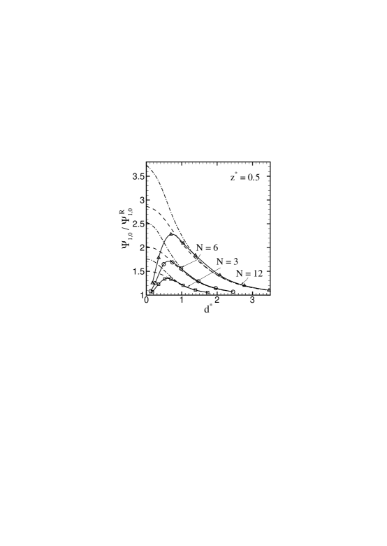
Figure 3: Ratio of the zero shear rate first normal stress difference coefficient in the presence of excluded volume interactions to the zero shear rate first normal stress difference coefficient in the Rouse model versus $d^{*}$, at a constant value of $z^{*}$, for three different values of $N$. The symbols are as indicated in the caption to Figure 1. The error bars in the Brownian dynamics simulations are smaller than the size of the symbols, and the continuous curves through the symbols are drawn for guiding the eye.

Figure 4: Equilibrium swelling of the end-to-end vector versus the re-scaled extent of excluded volume interaction $d=d^{*}/\sqrt{N}$, at a constant value of the re-scaled strength of the interaction $z={z^{*}}\sqrt{N}$, for three different values of $N$. The squares, circles and triangles represent the results of Brownian dynamics simulations for $N$ equal to 6, 12 and 24 beads, respectively. The continuous, dashed, and dot-dashed curves are the approximate predictions of the Gaussian approximation for $N$ equal to 6, 12 and 24 beads, respectively. The error bars in the Brownian dynamics simulations are smaller than the size of the symbols.

Figure 5: Swelling of the radius of gyration versus $d$, at a constant value of $z$, for three different values of $N$. The symbols are as indicated in the caption to Figure 4. The error bars in the Brownian dynamics simulations are smaller than the size of the symbols.

Figure 6: Ratio of the zero shear rate first normal stress difference coefficient in the presence of excluded volume interactions to the zero shear rate first normal stress difference coefficient in the Rouse model versus $d$, at a constant value of $z$, for three different values of $N$. The symbols are as indicated in the caption to Figure 4.

Figure 7: Equilibrium swelling of the end-to-end vector versus $d$, at a constant value of $z$, for different $N$. The continuous and dotted curves are the predictions of the Gaussian approximation for $N$ equal to 36 and 40 beads, respectively. The filled squares are the asymptotic predictions of the Gaussian approximation, obtained by numerical extrapolation of finite chain data to the limit of infinite chain length. The dashed and dot-dashed curves are the predictions of the first order perturbation theory for $N$ equal to 500 and 1000 beads, respectively. The filled diamonds are the predictions of the first order perturbation theory in the long chain limit, obtained by carrying out the integrals in eq 67 analytically. The circles, with error bars, are the results of Brownian dynamics simulations for $N=24$.

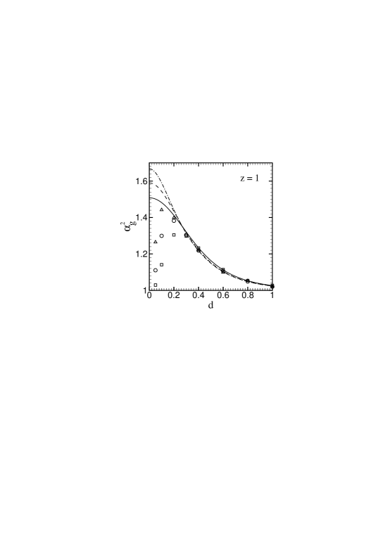
Figure 8: Swelling of the radius of gyration versus $d$, at two values of $z$, for three different values of $N$. The squares, circles and triangles (filled for $z=5$ and empty for $z=10$) represent the results of Brownian dynamics simulations for $N$ equal to 6, 12 and 24 beads, respectively. The continuous, dashed, and dot-dashed curves are the approximate predictions of the Gaussian approximation for $N$ equal to 6, 12 and 24 beads, respectively. The error bars in the Brownian dynamics simulations are smaller than the size of the symbols.

Figure 9: Ratio of the zero shear rate first normal stress difference coefficient in the presence of excluded volume interactions to the zero shear rate first normal stress difference coefficient in the Rouse model versus $d$, at two values of $z$, for three different values of $N$. The symbols are as indicated in the caption to Figure 8. The error bars in the Brownian dynamics simulations are smaller than the size of the symbols.

7 Equilibrium Swelling and Zero Shear Rate
Viscometric Functions

The prediction of equilibrium properties and zero shear rate viscometric functions, by Brownian dynamics simulations, the Gaussian approximation and the first order perturbation expansion, are compared in this section. Before doing so, it is appropriate to note that an equilibrium property, frequently defined in static theories of polymer solutions, namely, the swelling of the radius of gyration, $\alpha^{2}_{g}$, can be found from the following expression,

$$\alpha^{2}_{g}={{\bigl{\langle}}R_{g}^{2}\,{\bigr{\rangle}}_{\rm eq}\over{\bigl{\langle}}R_{g}^{2}\,{\bigr{\rangle}}_{\rm eq}^{R}}={\eta_{p,0}\over\eta_{p,0}^{R}}$$ (69)

because of the relation between the radius of gyration and the zero shear rate viscosity, eq 28. Plots of $\alpha^{2}_{g}$ in this section must, therefore, also be seen as plots of the ratio of the zero shear rate viscosity in the presence of excluded volume interactions to the zero shear rate viscosity in the Rouse model.

Figures 1 to 3 are plots of $\alpha^{2}$, $\alpha^{2}_{g}$ and $(\Psi_{1,0}/\Psi_{1,0}^{R})$ versus $d^{*}$, respectively, at a constant value of $z^{*}=0.5$, for three different chain lengths, $N=3$, $N=6$ and $N=12$. The squares, circles and triangles are exact results of Brownian dynamics simulations for the narrow Gaussian potential, the dashed lines are the predictions of the Gaussian approximation, and the dot-dashed curves are the predictions of the first order perturbation theory.

In the limit $d^{*}\to 0$ and for large values of $d^{*}$, for all the values of chain length $N$, the Brownian dynamics simulations reveal that equilibrium and zero shear rate properties tend to Rouse model values. In the case of $\alpha^{2}$ and $\alpha^{2}_{g}$, this is expected because of the rigorous result, eq 33. An immediate implication of this behavior is that, for chains of arbitrary but finite length, it is not fruitful to use a $\delta$-function potential to represent excluded volume interactions. On the other hand, the figures seem to suggest that a finite range of excluded volume interaction is required to cause an increase from Rouse model values. Both the first order perturbation theory and the Gaussian approximation predict a significant change from Rouse model values in the limit $d^{*}\to 0$. In the case of a dumbbell model, we were able to rigorously understand the origin of these spurious results [7]. The incorrect term-by-term integration of a series that was not uniformly convergent was found to be the source of the problem. Since first order perturbation theory is the basis for renormalisation group calculations, the invalidity of the $\delta$-function potential, which is frequently used in these calculations, is at first sight worrisome. However, we shall see below that the use of a $\delta$-function potential may be legitimate when both the limits, $N\to\infty$ and $d^{*}\to 0$, are considered.

Figures 1 to 3 show that there exists a threshold value of $d^{*}$ at which, the results of the Gaussian approximation and the first order perturbation theory, first agree with exact Brownian dynamics simulations. This is consistent with the first order perturbation theory predictions of the end-to-end vector, eq 65, and the viscometric functions, eqs 58 and 59, which reveal that, excluded volume corrections to the Rouse model decrease with increasing values of $d^{*}$. The threshold value of $d^{*}$ at which the approximations become accurate, increases as $N$ increases. This is a consequence of the well known result, which was demonstrated in section 6, that excluded volume corrections scale as ${z^{*}}\,\sqrt{N}$. Note, however, that the Gaussian approximation always becomes accurate at a smaller threshold value of $d^{*}$ than the first order perturbation theory. The Gaussian approximation, while being a non-perturbative approximation, is nevertheless, exact to first order in $z^{*}$. Consequently, as mentioned earlier, it might be considered to consist of an infinite number of higher order terms, and can be expected to be more accurate than the results of the first order perturbation theory.

All the results in Figures 1 to 3 are entirely consistent with the results obtained earlier with a dumbbell model for the polymer molecule. However, in the case of the dumbbell model, the dependence of the quality of the approximations on the chain length $N$, could not be examined. The results in Figures 1 to 3 seem to suggest that the Gaussian approximation has a rather limited validity, since for a given value of $z^{*}$ and $d^{*}$, it gets progressively worse as the chain length $N$ increases. This is in fact not a realistic picture—as is revealed below—when the data is reinterpreted in terms of a different set of coordinates.

Figures 4 to 6 are plots of $\alpha^{2}$, $\alpha^{2}_{g}$ and $(\Psi_{1,0}/\Psi_{1,0}^{R})$ versus $d=(d^{*}/\sqrt{N})$, respectively, at a constant value of $z={z^{*}}\sqrt{N}=1.0$, for three different chain lengths, $N=6$, $N=12$ and $N=24$. Before we discuss the figures, it is appropriate to make a few remarks about the choice of the variables in terms of which the data are displayed. Firstly, we choose $z$ as the measure of the strength of excluded volume interaction because perturbation theory clearly reveals that excluded volume corrections scale as ${z^{*}}\,\sqrt{N}$. A constant value of $z$, as $N$ increases, implies that ${z^{*}}$ must simultaneously decrease in order to keep the relative role of excluded volume interactions the same. Secondly, we choose the $x$-axis coordinate as $d=(d^{*}/\sqrt{N})$, because, as was shown in section 6, perturbation theory in the limit of long chains indicates that when the data is displayed in terms of $d$ and $z$, all the curves should collapse on to a single curve as $N\to\infty$. The parameter $d$ may be considered to be the extent of excluded volume interaction, measured as a fraction of the unperturbed (i.e., Rouse) root mean square end-to-end vector $\sqrt{{\bigl{\langle}}{{\mbox{\boldmath$r$}}}^{2}\,{\bigr{\rangle}}_{\rm eq}^{R}}$.

We first discuss the results of exact Brownian dynamics simulations displayed in Figures 4 to 6. As in Figures 1 to 3, all the properties start at Rouse values at $d=0$, go through a maximum as $d$ increases, and then finally decrease once more towards Rouse values with the continued increase of $d$. However, as the chain length increases, the values seem to rise increasingly more rapidly from the Rouse values at $d=0$, towards the maximum value. In other words, the slope at the origin seems to be getting steeper as $N$ increases. Indeed, the trend of the data leads one to speculate that, in the limit $N\to\infty$, the data might be singular at $d=0$, and consequently legitimize, in this limit, the use of a $\delta$-function excluded volume potential. This conclusion is of course only speculative, and needs to be established more rigorously. It has not been possible to examine more closely, with the help of Brownian dynamics simulations, the behavior at small values of $d$ for larger values of $N$, because of the excessive CPU time that is required. In terms of the non-dimensional time $t^{*}=(t/\lambda_{H})$, for $N=24$, a run for two non-dimensional time steps $\Delta t^{*}=0.1$ and $\Delta t^{*}=0.08$, required roughly 65 hours of CPU time on a SGI Origin2000 with a 195 MHz processor.

When viewed in terms of $z$ and $d$, the Gaussian approximation is revealed to be far more satisfactory than appeared at first sight in Figures 1 to 3. Indeed, for relatively small values of $d$, where the Gaussian approximation is inaccurate at small values of chain length, the Gaussian approximation seems to be becoming more accurate as $N$ increases. One might expect that as $N\to\infty$, the Gaussian approximation becomes accurate for an increasingly larger range of $d$ values. However, as will perhaps become clearer with the results discussed below, it appears that, for a given value of $z$, there exists a threshold value of $d$, below which the Gaussian approximation will be inaccurate, no matter how large a choice of $N$ is made. The reason for this behavior is related to a feature that is just noticeable in these figures—curves for different values of $N$ appear to be converging to an asymptote. This feature will become much clearer in Figure 7, and will be discussed in greater detail below.

For the sake of clarity, the predictions of the first order perturbation theory are not displayed in Figures 4 to 6. In contrast to the situation in Figures 1 to 3, where the accuracy of the first order perturbation theory becomes progressively worse as $N$ increases, its accuracy appears frozen when viewed in terms of $z$ and $d$. In other words, for different—sufficiently large—values of $N$, the first order perturbation theory first becomes accurate at the same threshold value of $d$. As in the case of the predictions of the Gaussian approximation, curves for different values of $N$ appear to be converging to a common asymptote. This can be seen clearly in Figure 7.

Figure 7 displays plots of $\alpha^{2}$ versus $d$, for different chain lengths, at a constant value of $z=1$. It clearly reveals the fact that, both in the Gaussian approximation and in the first order perturbation theory, curves for different values of $N$ collapse on to a single curve in the limit $N\to\infty$. A similar approach to an asymptotic limit is observed as $N\to\infty$, in the predictions of $\alpha^{2}_{g}$ and $(\Psi_{1,0}/\Psi_{1,0}^{R})$ by both the approximations, when they are plotted versus $d$. The results of Brownian dynamics simulations for $N=24$ are also plotted in Figure 7. They indicate that for $z=1$, asymptotic values have already been reached by Brownian dynamics simulations, at this relatively small value of $N$, for $d\geq 0.3$. One expects that as $N$ increases, asymptotic values will be reached for smaller and smaller values of $d$.

The asymptotic values predicted by the first order perturbation theory were obtained by carrying out the integrals in eq 67 analytically. It is worth noting that the convergence to the asymptotic value is quite slow as $d\to 0$. On the other hand, the asymptotic values predicted by the Gaussian approximation were obtained by a numerical procedure, as discussed below.

In the Gaussian approximation, calculation of the equilibrium and zero shear rate quantities requires the evaluation of the equilibrium moments $f_{jk}$. These are found here, as mentioned in appendix B, by numerical integration of the system of ordinary differential equations, eq 77, using a simple Euler scheme, until steady state is reached (the symmetry in $j$ and $k$ is used to reduce the number of equations by a factor of two). In addition, the evaluation of $\eta_{p,0}$ and $\Psi_{1,0}$ requires the inversion of the $(N-1)^{2}\times(N-1)^{2}$ matrix ${\overline{A}}_{jk,\,mn}$ (see eqs 90 and 91). As a result, the CPU time scales as $N^{6}$, and makes the task of generating data for large values of $N$ extremely computationally intensive. We have explored the predictions of chains up to a maximum of $N=40$, since for this value of $N$, a single run on the SGI Origin2000 computer required approximately 54 hours of CPU time. The asymptotic values in Figure 7 were obtained by the following procedure. For $z=1$, equilibrium and zero shear rate data, consisting of property values at different pairs of values $(d,N)$, were first compiled by performing a large number of runs for various values of $N$ as a function of $d$. A specific value of $d$ was then chosen, and assuming that the various properties were functions of $1/\sqrt{N}$, the values for different $N$ were extrapolated to the limit $N\to\infty$ using a rational function extrapolation algorithm [19]. The choice of $1/\sqrt{N}$ is motivated by the fact that the leading correction to the integrals in eq 67 is of order $1/\sqrt{N}$ [10].

The quality of Gaussian approximation as a function of the variable $z$, for the quantities $\alpha^{2}_{g}$ and $(\Psi_{1,0}/\Psi_{1,0}^{R})$, is displayed in Figures 8 and 9, respectively. The behavior of $\alpha^{2}$ has not been displayed as it is very similar to that of $\alpha^{2}_{g}$. It is clear from these figures that for a given value of $N$, the threshold value of $d$ beyond which the Gaussian approximation is accurate increases as $z$ increases. On the other hand, as in the case of $z=1$, for a fixed value of $z$, the accuracy of the Gaussian approximation seems to be increasing with $N$, for small values of $d$. There is, however, clearly a limit to this accuracy. As $N$ becomes large, the results of the exact Brownian dynamics simulations and the Gaussian approximation approach asymptotic values, and consequently, no further change can be noticed with changing $N$. Figures 8 and 9 seem to indicate that at small values of $d$, while the asymptotic values of Brownian dynamics simulations lie below the asymptotic values of the Gaussian approximation for $\alpha^{2}_{g}$, the opposite is true for $(\Psi_{1,0}/\Psi_{1,0}^{R})$. A clearer picture would be obtained if it were possible to carry out Brownian dynamics simulations with larger values of $N$.

Typical experimental values of $z$ lie in the range $0\leq z\leq 15$ [10]. As we have seen above, for large enough values of $d$, the Gaussian approximation remains accurate for a significant fraction of values of $z$ in this range. Since corrections to the Rouse model due to excluded volume interactions decrease with increasing shear rate, we can anticipate that the accuracy of the Gaussian approximation will improve as the shear rate increases. Furthermore, since the Gaussian approximation is extremely accurate for the treatment of hydrodynamic interaction effects, and since hydrodynamic interaction is likely to be the dominant effect in a combined theory of hydrodynamic interaction and excluded volume [20], it is perhaps fair to say that the results obtained so far clearly indicate the practical usefulness of the Gaussian approximation.

8 Conclusions

The influence of excluded volume interactions on the linear viscoelastic properties of a dilute polymer solution has been studied with the help of a narrow Gaussian excluded volume potential that acts between pairs of beads in a bead-spring chain model for the polymer molecule. Exact predictions of the model have been obtained by carrying out Brownian dynamics simulations, and approximate predictions have been obtained by two methods—firstly, by carrying out a first order perturbation expansion in the strength of excluded volume interaction, and secondly, by introducing a Gaussian approximation for the configurational distribution function.

The most appropriate way to represent the results of model calculations has been shown to be in terms of a suitably normalized strength of excluded volume interaction $z$, and a suitably normalized extent of excluded volume interaction $d$. When the results are viewed in terms of these variables, the following conclusions can be drawn:

1. The use of a $\delta$-function excluded volume potential (which is the narrow Gaussian excluded volume potential in the limit $d\to 0$) is not fruitful for chains with an arbitrary, but finite, number of beads $N$, because it leads to the prediction of properties identical to the Rouse model. The narrow Gaussian potential with a finite, non-zero, extent of interaction $d$, on the other hand, causes a swelling of the polymer chain at equilibrium, and an increase in the zero shear rate properties from their Rouse model values.

2. Curves for different—but sufficiently large—values of chain length $N$, collapse on to a unique asymptotic curve in the limit $N\to\infty$. The manner in which the results of Brownian dynamics simulations approach the asymptotic behavior indicates that there might be a singularity at $d=0$, and consequently, the use of a $\delta$-function excluded volume potential might be justified in the limit of infinite chain length.

3. The accuracy of the first order perturbation expansion becomes independent of $N$ for large $N$. For a given value of $z$, there exists a threshold value of $d$ beyond which the results of the first order perturbation theory agree with the exact results of Brownian dynamics simulations.

4. As in the case of the first order perturbation expansion, there exists a threshold value of $d$ beyond which the results of the Gaussian approximation agree with exact results. For a given value of $z$, this threshold value for accuracy is smaller than the threshold value in the first order perturbation theory. The accuracy of the Gaussian approximation decreases with increasing values of $z$.

Explicit expressions for the end-to-end vector and the viscometric functions in terms of the model parameters, obtained by carrying out a first order perturbation expansion, enable one to understand the behavior of the Gaussian approximation. This is because the Gaussian approximation is shown here to be exact to first order in $z$.

The accuracy of the Gaussian approximation, for a given value of $z$ and $d$, is expected to improve as the shear rate increases. This follows from the fact that corrections to the Rouse model, due to excluded volume interactions, decrease with increasing shear rate. Viscometric functions at non-zero shear rate predicted by Brownian dynamics simulations, the Gaussian approximation, and the first order perturbation expansion, will be compared in a subsequent publication.

The advantage of using the narrow Gaussian potential to represent excluded volume interactions is that the accuracy of approximate solutions can be assessed by comparison with exact results. This is in contrast with the situation for approximate renormalisation group calculations based on a $\delta$-function excluded volume potential, whose accuracy can only be judged by comparison with experiment, or with Monte Carlo simulations based on a different excluded volume potential.

The results obtained here indicate that the Gaussian approximation is an accurate approximation for describing excluded volume interactions, albeit within a certain range of parameter values. Since the usefulness of the Gaussian approximation has already been established for the treatment of hydrodynamic interactions, it is clearly worthwhile to examine the quality of the Gaussian approximation in a model for the combined effects of hydrodynamic interaction and excluded volume.

Acknowledgement. Support for this work through a grant III. 5(5)/98-ET from the Department of Science and Technology, India, is acknowledged. A significant part of this work was carried out while the author was an Alexander von Humboldt fellow at the Department of Mathematics, University of Kaiserslautern, Germany. The author would like to thank Professor H. C. Öttinger for carefully reading the manuscript, and for helpful suggestions. Thanks are also due to the High Performance Computational Facility at the University of Kaiserslautern for providing the use of their computers.

Appendix A $P_{\rm eq}({{\mbox{\boldmath$r$}}}_{\nu\mu})$ in the limit ${\tilde{d}}\to 0$ or ${\tilde{d}}\to\infty$

Upon substituting eq 14 and the Fourier representation of a $\delta$-function into eq 30, and rearranging terms, one obtains,

$$P_{\rm eq}({{\mbox{\boldmath$r$}}}_{\nu\mu})={1\over(2\pi)^{3}}\int\!\!d{{\mbox{\boldmath$k$}}}\,e^{i\,{{\mbox{\boldmath$r$}}}_{\nu\mu}\cdot{{\mbox{\boldmath$k$}}}}\left\{{\cal N_{\rm eq}}\int\!\!d{{{\mbox{\boldmath$Q$}}}}_{1}\ldots d{{{\mbox{\boldmath$Q$}}}}_{N-1}\,e^{-\left[\left(\phi/k_{\rm B}T\right)+i\left(\sum_{j=\mu}^{\nu-1}{{\mbox{\boldmath$Q$}}}_{j}\right)\cdot{{\mbox{\boldmath$k$}}}\right]}\right\}$$ (70)

We now consider the integral within braces on the right hand side of eq 70, and take up the integration over the bead connector vector ${{\mbox{\boldmath$Q$}}}_{1}$. Separating out all the terms containing the vector ${{\mbox{\boldmath$Q$}}}_{1}$, we can rewrite this integral as,

$${\cal N_{\rm eq}}\int\!\!d{{{\mbox{\boldmath$Q$}}}}_{2}\ldots d{{{\mbox{\boldmath$Q$}}}}_{N-1}\,\exp\biggl{[}-{H\over 2k_{\rm B}T}\sum_{j=2}^{N-1}{{\mbox{\boldmath$Q$}}}_{j}^{2}-i\left(\sum_{j=\mu}^{\nu-1}(1-\delta_{1j})\,{{\mbox{\boldmath$Q$}}}_{j}\right)\cdot{{\mbox{\boldmath$k$}}}$$

$$-{1\over 2k_{\rm B}T}\sum_{\alpha,\beta=2\atop\alpha\neq\beta}^{N}\,E\left({{{\mbox{\boldmath$r$}}}}_{\alpha}-{{{\mbox{\boldmath$r$}}}}_{\beta}\right)\biggr{]}\,\Biggl{\{}\int\!\!d{{{\mbox{\boldmath$Q$}}}}_{1}\,\exp\biggl{[}-{H\over 2k_{\rm B}T}\,{{\mbox{\boldmath$Q$}}}_{1}^{2}-i\,\delta_{1\mu}\,{{\mbox{\boldmath$Q$}}}_{1}\cdot{{\mbox{\boldmath$k$}}}$$

$$-{1\over k_{\rm B}T}\,\left[E\left({{{\mbox{\boldmath$r$}}}}_{1}-{{{\mbox{\boldmath$r$}}}}_{2}\right)+E\left({{{\mbox{\boldmath$r$}}}}_{1}-{{{\mbox{\boldmath$r$}}}}_{3}\right)+\ldots+E\left({{{\mbox{\boldmath$r$}}}}_{1}-{{{\mbox{\boldmath$r$}}}}_{N}\right)\right]\biggr{]}\Biggr{\}}$$ (71)

where, a typical term of the excluded volume potential contribution to the ${{\mbox{\boldmath$Q$}}}_{1}$ integral, has the form,

$$E\left({{{\mbox{\boldmath$r$}}}}_{1}-{{{\mbox{\boldmath$r$}}}}_{\beta}\right) = {v\,k_{\rm B}T\over[2\pi{\tilde{d}}^{2}]^{3\over 2}}\,\exp\Biggl{\{}-{1\over 2{\tilde{d}}^{2}}\,\biggl{(}{{\mbox{\boldmath$Q$}}}_{1}^{2}+2\,{{\mbox{\boldmath$Q$}}}_{1}\cdot{{\mbox{\boldmath$r$}}}_{\beta 2}+{{\mbox{\boldmath$Q$}}}_{2}^{2}+2\,{{\mbox{\boldmath$Q$}}}_{2}\cdot{{\mbox{\boldmath$r$}}}_{\beta 3}+\ldots$$

$$+ {{\mbox{\boldmath$Q$}}}_{\beta-2}^{2}+2\,{{\mbox{\boldmath$Q$}}}_{\beta-2}\cdot{{\mbox{\boldmath$r$}}}_{\beta,\,\beta-1}+{{\mbox{\boldmath$Q$}}}_{\beta-1}^{2}\biggr{)}\Biggr{\}}$$

We now convert the ${{\mbox{\boldmath$Q$}}}_{1}$ integral into spherical coordinates. In order to do so, we need to choose a reference vector to fix a direction in space. In the ${{\mbox{\boldmath$Q$}}}_{1}$ integration, all the other vectors, ${{\mbox{\boldmath$Q$}}}_{2},\ldots,{{\mbox{\boldmath$Q$}}}_{N-1}$ and $k$ are fixed. Without loss of generality, we choose the fixed vector as ${{\mbox{\boldmath$Q$}}}_{2}$, denote its direction as the $z$ direction, and choose, in the plane perpendicular to ${{\mbox{\boldmath$Q$}}}_{2}$, an arbitrary pair of orthogonal directions as the $x$ and $y$ axes. Let, $\theta_{1}$, $\theta_{\beta 2}$, and $\theta_{k}$ represent the angles that the vectors ${{\mbox{\boldmath$Q$}}}_{1}$, ${{\mbox{\boldmath$r$}}}_{\beta 2}$ and $k$ make with the $z$ direction, respectively. Similarly, let $\phi_{1}$, $\phi_{\beta 2}$, and $\phi_{k}$ represent the angles that the projections of these vectors on the $xy$ plane, make with the $x$ direction. Then,

$${{\mbox{\boldmath$Q$}}}_{1}\cdot{{\mbox{\boldmath$r$}}}_{\beta 2}=Q_{1}\,r_{\beta 2}\,F_{\beta 2}\,(\theta_{1},\phi_{1})$$

where, $Q_{1}$ and $r_{\beta 2}$ represent the magnitudes of ${{\mbox{\boldmath$Q$}}}_{1}$ and ${{\mbox{\boldmath$r$}}}_{\beta 2}$, respectively, and,

$$F_{\beta 2}\,(\theta_{1},\phi_{1})=\sin\theta_{1}\sin\theta_{\beta 2}(\cos\phi_{1}\cos\phi_{\beta 2}+\sin\phi_{1}\sin\phi_{\beta 2})+\cos\theta_{1}\cos\theta_{\beta 2}$$

Defining the function $F_{k}\,(\theta_{1},\phi_{1})$ similarly, we can rewrite the ${{\mbox{\boldmath$Q$}}}_{1}$ integral in expression 71, in terms of spherical coordinates as,

$$I_{Q_{1}}=\int_{0}^{\infty}\!\!dQ_{1}\int_{0}^{2\pi}\!\!d\theta_{1}\int_{0}^{\pi}\!\!d\phi_{1}\,Q_{1}^{2}\,\sin\theta_{1}\,\exp\left[-{H\over 2k_{\rm B}T}\,Q_{1}^{2}-i\,\delta_{1\mu}\,Q_{1}k\,F_{k}\,(\theta_{1},\phi_{1})\right]\times$$

$$\exp\,\Biggl{\{}-{1\over k_{\rm B}T}\,\Biggl{[}{v\,k_{\rm B}T\over\left(2\pi{\tilde{d}}^{2}\right)^{3/2}}\,\biggl{\{}e^{-{1\over 2{\tilde{d}}^{2}}\,Q_{1}^{2}}+e^{-{1\over 2{\tilde{d}}^{2}}\left(Q_{1}^{2}+2\,Q_{1}\,r_{32}\,F_{32}(\theta_{1},\phi_{1})\,\right)}\,e^{-{1\over 2{\tilde{d}}^{2}}\,{{\mbox{\boldmath$Q$}}}_{2}^{2}}$$

$$+\ldots+e^{-{1\over 2{\tilde{d}}^{2}}\left(Q_{1}^{2}+2\,Q_{1}\,r_{N2}\,F_{N2}(\theta_{1},\phi_{1})\,\right)}\,e^{-{1\over 2{\tilde{d}}^{2}}\,\left({{\mbox{\boldmath$Q$}}}_{2}^{2}+2\,{{\mbox{\boldmath$Q$}}}_{2}\cdot{{\mbox{\boldmath$r$}}}_{N3}+\ldots+{{\mbox{\boldmath$Q$}}}_{N-1}^{2}\right)}\biggr{\}}\,\Biggr{]}\,\Biggr{\}}$$ (72)

For $Q_{1}=0$, the integrand is identically zero. For $Q_{1}\neq 0$, in the limit ${\tilde{d}}\to 0$ or ${\tilde{d}}\to\infty$, the integrand tends to,

$$Q_{1}^{2}\,\sin\theta_{1}\,\exp\left\{-{H\over 2k_{\rm B}T}\,Q_{1}^{2}-i\,\delta_{1\mu}\,Q_{1}k\,F_{k}\,(\theta_{1},\phi_{1})\right\}$$

The integrand is also a bounded function of $Q_{1}$ for all values ${\tilde{d}}$.

An argument similar to the one above can be carried out for each of the remaining integrations over ${{\mbox{\boldmath$Q$}}}_{2},\ldots,{{\mbox{\boldmath$Q$}}}_{N-1}$. It follows that,

$$\lim_{{\tilde{d}}\to 0\atop{\rm or},\,{\tilde{d}}\to\infty}\int\!\!d{{{\mbox{\boldmath$Q$}}}}_{1}\ldots d{{{\mbox{\boldmath$Q$}}}}_{N-1}\,\exp\left\{-\left({\phi\over k_{\rm B}T}\right)-i\left(\sum_{j=\mu}^{\nu-1}{{\mbox{\boldmath$Q$}}}_{j}\right)\cdot{{\mbox{\boldmath$k$}}}\right\}$$

$$=\int\!\!d{{{\mbox{\boldmath$Q$}}}}_{1}\ldots d{{{\mbox{\boldmath$Q$}}}}_{N-1}\,\exp\left\{-\left({H\over 2k_{\rm B}T}\right)\sum_{j=1}^{N-1}{{\mbox{\boldmath$Q$}}}_{j}^{2}-i\left(\sum_{j=\mu}^{\nu-1}{{\mbox{\boldmath$Q$}}}_{j}\right)\cdot{{\mbox{\boldmath$k$}}}\right\}$$ (73)

With regard to the normalization factor $\cal N_{\rm eq}$, since,

$${\cal N}_{\rm eq}=\left[\int\!\!d{{{\mbox{\boldmath$Q$}}}}_{1}\ldots d{{{\mbox{\boldmath$Q$}}}}_{N-1}\,\exp\left(-{\phi\over k_{\rm B}T}\right)\right]^{-1}$$ (74)

we can show, by adopting a procedure similar to that above that,

$$\lim_{{\tilde{d}}\to 0\atop{\rm or},\,{\tilde{d}}\to\infty}{\cal N}_{\rm eq}={\cal N}_{\rm eq}^{R}$$ (75)

As a result, we have established that,

$$\lim_{{\tilde{d}}\to 0\atop{\rm or},\,{\tilde{d}}\to\infty}P_{\rm eq}({{\mbox{\boldmath$r$}}}_{\nu\mu}) = {1\over(2\pi)^{3}}\int\!\!d{{\mbox{\boldmath$k$}}}\,e^{i\,{{\mbox{\boldmath$r$}}}_{\nu\mu}\cdot{{\mbox{\boldmath$k$}}}}\,\,\Biggl{\{}\int\!\!d{{{\mbox{\boldmath$Q$}}}}_{1}\ldots d{{{\mbox{\boldmath$Q$}}}}_{N-1}\,\psi_{\rm eq}^{R}\,e^{-\,i\left[\sum_{j=\mu}^{\nu-1}{{\mbox{\boldmath$Q$}}}_{j}\right]\cdot{{\mbox{\boldmath$k$}}}}\,\Biggr{\}}$$ (76)

$$= P_{\rm eq}^{R}({{\mbox{\boldmath$r$}}}_{\nu\mu})$$

Appendix B Codeformational Memory-Integral Expansion

Upon expanding the tensors ${{{\mbox{\boldmath$\sigma\!$}}}_{jk}}$ in the manner displayed in eq 46, substituting the expansion into the second moment equation, eq 43, and separating the resultant equation into equations for each order in the velocity gradient, the following two equations are obtained, Equilibrium:

$${d\over dt}\,f_{jk}={2k_{\rm B}T\over\zeta}\,A_{jk}-\left({H\over\zeta}\right)\,\sum_{m=1}^{N-1}\left[f_{jm}\,(A_{mk}-{z^{*}}\,\Delta^{(0)}_{km}\,)+(A_{jm}-{z^{*}}\,\Delta^{(0)}_{jm}\,)\,f_{mk}\right]$$ (77)

where,

$$\Delta^{(0)}_{jm}=\sum_{\mu=1}^{N}\left[\,{(B_{j+1,\,m}-B_{\mu m})\over\left({d^{*}}^{2}+{\hat{f}}_{j+1,\,\mu}\right)^{5/2}}-{(B_{jm}-B_{\mu m})\over\left({d^{*}}^{2}+{\hat{f}}_{j\mu}\right)^{5/2}}\,\right]$$ (78)

with the quantities ${\hat{f}}_{\nu\mu}$ given by,

$${\hat{f}}_{\nu\mu}=\left({H\over k_{B}T}\right)\,\sum_{j,k\,=\,\min(\mu,\nu)}^{\max(\mu,\nu)-1}\,f_{jk}$$ (79)

First Order:

$${d\over dt}\,{{\mbox{\boldmath$\epsilon$}}}_{jk}=({\mbox{\boldmath$\kappa$}}+{\mbox{\boldmath$\kappa$}}^{T})\,f_{jk}-\left({H\over\zeta}\right)\,\sum_{m,n=1}^{N-1}{\overline{A}}_{jk,\,mn}\,{{\mbox{\boldmath$\epsilon$}}}_{mn}$$ (80)

where,

$${\overline{A}}_{jk,\,mn}=(A_{jm}\,\delta_{kn}+\delta_{jm}\,A_{kn})-{z^{*}}\,(\Delta^{(0)}_{jm}\,\delta_{kn}+\delta_{jm}\,\Delta^{(0)}_{kn})$$

$$+{z^{*}}\,\left({H\over k_{B}T}\right)\,\sum_{p=1}^{N-1}\left[f_{jp}\,\Delta^{(1)}_{kp,\,mn}+\Delta^{(1)}_{jp,\,mn}\,f_{pk}\right]$$ (81)

with the quantities $\Delta^{(1)}_{jp,\,mn}$ given by,

$$\Delta^{(1)}_{jp,\,mn}=\sum_{\mu=1}^{N}\left[\,{(B_{j+1,\,p}-B_{\mu p})\,\theta(\mu,m,n,j+1)\over\left({d^{*}}^{2}+{\hat{f}}_{j+1,\,\mu}\right)^{7/2}}-{(B_{jp}-B_{\mu p})\,\theta(\mu,m,n,j)\over\left({d^{*}}^{2}+{\hat{f}}_{j\mu}\right)^{7/2}}\,\right]$$ (82)

The function $\theta(\mu,m,n,\nu)$ has been introduced previously in the treatment of hydrodynamic interaction [2]. It is unity if $m$ and $n$ lie between $\mu$ and $\nu$, and zero otherwise,

$$\theta(\mu,m,n,\nu)=\cases{1&if $\mu\leq m,n<\nu$ \quad or\quad$\nu\leq m,n<\mu$\cr\vskip 3.0pt\cr 0&otherwise\cr}$$ (83)

Introducing new indices for the pairs $(j,k)$ and $(m,n)$, the quantity ${\overline{A}}_{jk,\,mn}$ may be considered an $(N-1)^{2}\times(N-1)^{2}$ matrix. The inverse can then be defined in the following manner,

$$\sum_{r,s=1}^{N-1}{\overline{A}}^{\,-1}_{jk,\,rs}\,{\overline{A}}_{rs,\,mn}={{1\kern-2.79999pt{\rm I}}}_{jk,\,mn}$$ (84)

where, ${{1\kern-2.79999pt{\rm I}}}$ is the $(N-1)^{2}\times(N-1)^{2}$ unit matrix ${{1\kern-2.79999pt{\rm I}}}_{jk,\,mn}=\delta_{jm}\,\delta_{kn}$.

In the equilibrium second moment equation, eq 77, the term $(df_{jk}/dt)$ on the left hand side, is identically zero. It is retained here, however, to indicate that the equation is solved for $f_{jk}$ by numerical integration of the ODE’s until steady state is reached.

Upon integrating eq 80 with respect to time, and substituting the solution into eq 38, we finally obtain the expression, eq 47, for the first order codeformational memory-integral expansion, where, the memory function $G(t)$ is given by,

$$G(t)=\sum_{j,k=1}^{N-1}\,\sum_{m,n=1}^{N-1}f_{jm}\,{\cal H}_{jk}\,{\cal E}\biggl{[}\,-\,{t\over\lambda_{H}}\,{\widetilde{A}}\,\biggr{]}_{\,mk,\,nn}$$ (85)

In eq 85, $\lambda_{H}=(\zeta/4H)$ is the familiar time constant, ${\cal H}_{jk}$ is defined by,

$${\cal H}_{jk}=n_{\rm p}H\left[\delta_{jk}-{1\over 2}\,{z^{*}}\sum_{\mu,\nu=1\atop\mu\neq\nu}^{N}{{d^{*}}^{2}\over\left({d^{*}}^{2}+{\hat{f}}_{\nu\mu}\right)^{7/2}}\,\theta(\nu,j,k,\mu)\right]$$ (86)

and the quantity ${\widetilde{A}}_{jk,\,mn}$ is given by,

$${\widetilde{A}}_{jk,\,mn}=\sum_{r,s=1}^{N-1}{1\over 4}\,f^{-1}_{jr}\,{\overline{A}}_{rk,\,sn}\,f_{sm}$$ (87)

The exponential operator ${\cal E}\,[\,M\,]$ maps one matrix into another according to:

$${\cal E}\,[\,M\,]_{\,jk,\,mn}={{1\kern-2.79999pt{\rm I}}}_{jk,\,mn}+M_{jk,\,mn}+{1\over 2!}\sum_{r,s=1}^{N-1}\,M_{jk,\,rs}\,M_{rs,\,mn}+\ldots$$

and has the useful properties,

$${d\over dt}\,{\cal E}\,[\,Mt\,]_{\,jk,\,mn}=\sum_{r,s=1}^{N-1}M_{jk,\,rs}\,{\cal E}\,[\,Mt\,]_{\,rs,\,mn}=\sum_{r,s=1}^{N-1}{\cal E}\,[\,Mt\,]_{\,jk,\,rs}\,M_{rs,\,mn}$$

$$\sum_{r,s=1}^{N-1}{\cal E}\,[\,a\,M\,]_{\,jk,\,rs}\,\,{\cal E}\,[\,b\,{{1\kern-2.79999pt{\rm I}}}\,]_{\,rs,\,mn}={\cal E}\,[\,a\,M+b\,{{1\kern-2.79999pt{\rm I}}}\,]_{\,jk,\,mn}$$

for arbitrary constants $a$ and $b$.

As mentioned in section 5, once the memory function $G(s)$ is obtained, one can obtain the material functions in small amplitude oscillatory shear flow, and the zero shear rate viscometric functions. Following the procedure outlined in section 5, we can show that,

$$\eta^{\prime}(\omega) = \lambda_{H}\sum_{j,k=1}^{N-1}\,\sum_{m,n=1}^{N-1}\,\sum_{r,s=1}^{N-1}f_{jk}\,{\cal H}_{jm}\,\Phi^{-1}_{km,\,rs}\,{\widetilde{A}}_{rs,\,nn}$$

$$\eta^{\prime\prime}(\omega) = \lambda_{H}^{2}\,\omega\sum_{j,k=1}^{N-1}\,\sum_{m,n=1}^{N-1}f_{jk}\,{\cal H}_{jm}\,\Phi^{-1}_{km,\,nn}$$ (88)

where,

$$\Phi_{jk,\,mn}=\sum_{r,s=1}^{N-1}\left[{\widetilde{A}}_{jk,\,rs}\,{\widetilde{A}}_{rs,\,mn}+\lambda_{H}^{2}\,\omega^{2}{{1\kern-2.79999pt{\rm I}}}_{jk,\,mn}\right]$$ (89)

Using the relations between the zero shear rate viscometric functions and $\eta^{\prime}$ and $\eta^{\prime\prime}$ (eqs 51), one can show that,

$$\eta_{p,0} = 4\,\lambda_{H}\sum_{j,k=1}^{N-1}\,\sum_{m,n=1}^{N-1}{\cal H}_{jk}\,{\overline{A}}^{\,-1}_{jk,\,mn}\,f_{mn}$$ (90)

$$\Psi_{1,0} = 32\,\lambda_{H}^{2}\sum_{j,k=1}^{N-1}\,\sum_{m,n=1}^{N-1}\,\sum_{r,s=1}^{N-1}{\cal H}_{jk}\,{\overline{A}}^{\,-1}_{jk,\,mn}\,{\overline{A}}^{\,-1}_{mn,\,rs}\,f_{rs}$$ (91)

Appendix C Viscometric functions correct to first order in $z^{*}$

The first step in calculating the first order excluded volume corrections to the Rouse viscometric functions, as mentioned earlier, is to evaluate the time integrals in eqs 52 and 57. These time integrals can be carried out by using the forms of the tensors ${{{\mbox{\boldmath$\gamma$}}}}_{[1]}$ and $E$ in steady shear flow, tabulated in reference 12. One can show that the expression for the second moment ${{\mbox{\boldmath$\sigma\!$}}}^{R}_{jk}$, which is required to explicitly evaluate all the averages carried out with the Rouse distribution function $\psi_{R}$, is given by,

$${{\mbox{\boldmath$\sigma\!$}}}^{R}_{jk}={k_{\rm B}T\over H}\left\{\delta_{jk}\,{{\mbox{\boldmath$1$}}}+2\lambda_{H}C_{jk}\left({\mbox{\boldmath$\kappa$}}+{\mbox{\boldmath$\kappa$}}^{T}\right)+8\lambda_{H}^{2}C^{2}_{jk}\left({\mbox{\boldmath$\kappa$}}\cdot{\mbox{\boldmath$\kappa$}}^{T}\right)\right\}$$ (92)

while the stress tensor in steady shear flow has the form,

$${{\mbox{\boldmath$\tau$}}}^{p} = -n_{\rm p}k_{B}T\sum_{j=1}^{N-1}\left[2\lambda_{H}\,C_{jj}\left({\mbox{\boldmath$\kappa$}}+{\mbox{\boldmath$\kappa$}}^{T}\right)+8\lambda_{H}^{2}\,C^{2}_{jj}\left({\mbox{\boldmath$\kappa$}}\cdot{\mbox{\boldmath$\kappa$}}^{T}\right)\right]$$ (93)

$$- n_{\rm p}H\sum_{j,k=1}^{N-1}\biggl{\{}2\lambda_{H}\,C_{kj}\,{{\mbox{\boldmath$Y$}}}^{R}_{jk}+4\lambda_{H}^{2}\,C^{2}_{kj}\left[{\mbox{\boldmath$\kappa$}}\cdot{{\mbox{\boldmath$Y$}}}^{R}_{jk}+{{\mbox{\boldmath$Y$}}}^{R}_{jk}\cdot{\mbox{\boldmath$\kappa$}}^{T}\right]$$

$$+ 16\lambda_{H}^{3}\,C^{3}_{kj}\left[{\mbox{\boldmath$\kappa$}}\cdot{{\mbox{\boldmath$Y$}}}^{R}_{jk}\cdot{\mbox{\boldmath$\kappa$}}^{T}\right]\biggr{\}}+{{\mbox{\boldmath$Z$}}}^{R}$$

A similar expression, without the ${{\mbox{\boldmath$Z$}}}^{R}$ term, has been derived by Öttinger [17] in his renormalisation group treatment of excluded volume effects—within the framework of polymer kinetic theory—using a $\delta$-function excluded volume potential.

Table 1: Functions, appearing in eq 94, representing the indirect excluded volume contributions to the stress tensor in steady shear flow. The quantity $\Omega$ is defined by, $\Omega=4/({d^{*}}^{2}+S_{\mu\nu}^{(0)})^{2}$.

$\alpha^{(0)}_{\mu\nu}=\lambda_{H}\,S_{\mu\nu}^{(0)}\,\Omega\left[\left({d^{*}}^{2}+S_{\mu\nu}^{(0)}\right)^{2}+\lambda_{H}^{2}{\dot{\gamma}}^{2}\,\left\{2\,S_{\mu\nu}^{(2)}\left({d^{*}}^{2}+S_{\mu\nu}^{(0)}\right)-S_{\mu\nu}^{(1)}\,S_{\mu\nu}^{(1)}\right\}\right]$

$\alpha^{(1)}_{\mu\nu}=\lambda_{H}^{2}\,S_{\mu\nu}^{(1)}\,\Omega\left[\left({d^{*}}^{2}+S_{\mu\nu}^{(0)}\right)\left(2{d^{*}}^{2}+S_{\mu\nu}^{(0)}\right)+2\lambda_{H}^{2}{\dot{\gamma}}^{2}\left\{2\,S_{\mu\nu}^{(2)}\left({d^{*}}^{2}+S_{\mu\nu}^{(0)}\right)-S_{\mu\nu}^{(1)}\,S_{\mu\nu}^{(1)}\right\}\right]$

$\alpha^{(2)}_{\mu\nu}=\lambda_{H}^{3}\,\Omega\left[\,3\,{d^{*}}^{2}+2\,S_{\mu\nu}^{(0)}+6\lambda_{H}^{2}{\dot{\gamma}}^{2}\,S_{\mu\nu}^{(2)}+\,2\,S_{\mu\nu}^{(2)}\left({d^{*}}^{2}+S_{\mu\nu}^{(0)}\right)-S_{\mu\nu}^{(1)}\,S_{\mu\nu}^{(1)}\right]$

$\alpha^{(3)}_{\mu\nu}=-\lambda_{H}^{3}\,\Omega\,S_{\mu\nu}^{(1)}\,S_{\mu\nu}^{(1)}\,{d^{*}}^{2}$

$\alpha^{(4)}_{\mu\nu}=\lambda_{H}^{4}\,S_{\mu\nu}^{(1)}\,\Omega\left[\,2\,S_{\mu\nu}^{(1)}\,S_{\mu\nu}^{(1)}-3\,S_{\mu\nu}^{(2)}\left({d^{*}}^{2}+S_{\mu\nu}^{(0)}\right)\right]$

$\alpha^{(5)}_{\mu\nu}=\alpha^{(4)}_{\mu\nu}$

$\alpha^{(6)}_{\mu\nu}=2\,\lambda_{H}^{5}\,\Omega\left[\,3\,S_{\mu\nu}^{(2)}\left\{S_{\mu\nu}^{(1)}\,S_{\mu\nu}^{(1)}-S_{\mu\nu}^{(2)}\left({d^{*}}^{2}+S_{\mu\nu}^{(0)}\right)\right\}-2\,S_{\mu\nu}^{(3)}\,S_{\mu\nu}^{(1)}\left({d^{*}}^{2}+S_{\mu\nu}^{(0)}\right)\right]$

Table 2: Functions, appearing in eq 94, representing the direct excluded volume contributions to the stress tensor in steady shear flow. The quantity $\Omega$ is defined by, $\Omega=4/({d^{*}}^{2}+S_{\mu\nu}^{(0)})^{2}$.

$\beta^{(0)}_{\mu\nu}=\lambda_{H}\,S_{\mu\nu}^{(0)}\,\Omega\left[\left({d^{*}}^{2}+S_{\mu\nu}^{(0)}\right)^{2}+\lambda_{H}^{2}{\dot{\gamma}}^{2}\,\left\{2\,S_{\mu\nu}^{(2)}\left({d^{*}}^{2}+S_{\mu\nu}^{(0)}\right)-S_{\mu\nu}^{(1)}\,S_{\mu\nu}^{(1)}\right\}\right]$

$\beta^{(1)}_{\mu\nu}=\lambda_{H}^{2}\,S_{\mu\nu}^{(1)}\,\Omega\left[\left({d^{*}}^{2}+S_{\mu\nu}^{(0)}\right){d^{*}}^{2}+\lambda_{H}^{2}{\dot{\gamma}}^{2}\left\{2\,S_{\mu\nu}^{(2)}\left({d^{*}}^{2}+S_{\mu\nu}^{(0)}\right)-S_{\mu\nu}^{(1)}\,S_{\mu\nu}^{(1)}\right\}\right]$

$\beta^{(2)}_{\mu\nu}=\lambda_{H}^{3}\,\Omega\left[\,{d^{*}}^{2}+2\lambda_{H}^{2}{\dot{\gamma}}^{2}\,S_{\mu\nu}^{(2)}+\,2\,S_{\mu\nu}^{(2)}\left({d^{*}}^{2}+S_{\mu\nu}^{(0)}\right)-S_{\mu\nu}^{(1)}\,S_{\mu\nu}^{(1)}\right]$

$\beta^{(3)}_{\mu\nu}=-\lambda_{H}^{3}\,\Omega\,S_{\mu\nu}^{(1)}\,S_{\mu\nu}^{(1)}\,{d^{*}}^{2}$

$\beta^{(4)}_{\mu\nu}=\lambda_{H}^{4}\,S_{\mu\nu}^{(1)}\,\Omega\left[\,S_{\mu\nu}^{(1)}\,S_{\mu\nu}^{(1)}-2\,S_{\mu\nu}^{(2)}\left({d^{*}}^{2}+S_{\mu\nu}^{(0)}\right)\right]$

$\beta^{(5)}_{\mu\nu}=\beta^{(4)}_{\mu\nu}$

$\beta^{(6)}_{\mu\nu}=2\,\lambda_{H}^{5}\,\Omega\left[\,S_{\mu\nu}^{(1)}\,S_{\mu\nu}^{(1)}-2\,S_{\mu\nu}^{(2)}\left({d^{*}}^{2}+S_{\mu\nu}^{(0)}\right)\right]$

The next step is to explicitly evaluate the tensors ${{\mbox{\boldmath$Y$}}}_{jk}^{R}$ and ${{\mbox{\boldmath$Z$}}}^{R}$, in terms of the velocity gradient $\kappa$ and the Kramers matrix $C_{kj}$, by using eq 92 for ${{\mbox{\boldmath$\sigma\!$}}}^{R}_{jk}$. The resultant expressions are then substituted into eq 93, and after a lengthy calculation, the following explicit expression for the excluded volume contribution to the stress tensor, correct to first order in $z^{*}$, is obtained,

$${{\mbox{\boldmath$\tau$}}}^{p}_{(E)} = -{1\over 8\lambda_{H}}\,n_{\rm p}k_{B}T\,z^{*}\sum_{\mu,\nu=1\atop\mu\neq\nu}^{N}{1\over\left({d^{*}}^{2}+S_{\mu\nu}^{(0)}\right)^{5/2}\,e_{\mu\nu}({\dot{\gamma}})^{3/2}}\,\Biggl{\{}\left(\alpha_{\mu\nu}^{(0)}-\beta_{\mu\nu}^{(0)}\right){{\mbox{\boldmath$1$}}}$$ (94)

$$+ \left(\alpha_{\mu\nu}^{(1)}-\beta_{\mu\nu}^{(1)}\right)\left({\mbox{\boldmath$\kappa$}}+{\mbox{\boldmath$\kappa$}}^{T}\right)+\left(\alpha_{\mu\nu}^{(2)}-\beta_{\mu\nu}^{(2)}\right)\left({\mbox{\boldmath$\kappa$}}\cdot{\mbox{\boldmath$\kappa$}}^{T}\right)+\left(\alpha_{\mu\nu}^{(3)}-\beta_{\mu\nu}^{(3)}\right)\left({\mbox{\boldmath$\kappa$}}^{T}\cdot{\mbox{\boldmath$\kappa$}}\right)$$

$$+ \left(\alpha_{\mu\nu}^{(4)}-\beta_{\mu\nu}^{(4)}\right)\left({\mbox{\boldmath$\kappa$}}\cdot{\mbox{\boldmath$\kappa$}}^{T}\cdot{\mbox{\boldmath$\kappa$}}\right)+\left(\alpha_{\mu\nu}^{(5)}-\beta_{\mu\nu}^{(5)}\right)\left({\mbox{\boldmath$\kappa$}}^{T}\cdot{\mbox{\boldmath$\kappa$}}\cdot{\mbox{\boldmath$\kappa$}}^{T}\right)$$

$$+ \left(\alpha_{\mu\nu}^{(6)}-\beta_{\mu\nu}^{(6)}\right)\left({\mbox{\boldmath$\kappa$}}\cdot{\mbox{\boldmath$\kappa$}}^{T}\cdot{\mbox{\boldmath$\kappa$}}\cdot{\mbox{\boldmath$\kappa$}}^{T}\right)\Biggr{\}}$$

where, the functions $\alpha_{\mu\nu}^{(j)}$ and $\beta_{\mu\nu}^{(j)};\,(j=0,1,\ldots,6)$, which represent the indirect and direct contributions respectively, are given in Tables 1 and 2, and the function $e_{\mu\nu}({\dot{\gamma}})$ is defined by,

$$e_{\mu\nu}({\dot{\gamma}})=1+{\lambda_{H}^{2}{\dot{\gamma}}^{2}\over\left({d^{*}}^{2}+S_{\mu\nu}^{(0)}\right)^{2}}\left[2\left({d^{*}}^{2}+S_{\mu\nu}^{(0)}\right)S_{\mu\nu}^{(2)}-S_{\mu\nu}^{(1)}\,S_{\mu\nu}^{(1)}\right]$$ (95)

Equation 94 for the stress tensor can then be used to find the excluded volume contributions to the viscometric functions, correct to first order in $z^{*}$, by using the definitions in eqs 22,

$$\eta_{p}^{(E)} = {1\over 2}\,\lambda_{H}^{2}\,z^{*}\sum_{\mu,\nu=1\atop\mu\neq\nu}^{N}{1\over\left({d^{*}}^{2}+S_{\mu\nu}^{(0)}\right)^{7/2}e_{\mu\nu}({\dot{\gamma}})^{3/2}}\,\biggl{[}\,S_{\mu\nu}^{(0)}\,S_{\mu\nu}^{(1)}+\lambda_{H}^{2}{\dot{\gamma}}^{2}\,S_{\mu\nu}^{(1)}S_{\mu\nu}^{(2)}$$ (96)

$$+ {d^{*}}^{2}\,S_{\mu\nu}^{(1)}\,\biggr{]}$$

$$\Psi_{1}^{(E)} = \lambda_{H}^{2}\,z^{*}\sum_{\mu,\nu=1\atop\mu\neq\nu}^{N}{1\over\left({d^{*}}^{2}+S_{\mu\nu}^{(0)}\right)^{7/2}\,e_{\mu\nu}({\dot{\gamma}})^{3/2}}$$ (97)

$$\times \left[\,2\,S_{\mu\nu}^{(2)}\left({d^{*}}^{2}+S_{\mu\nu}^{(0)}\right)-S_{\mu\nu}^{(1)}\,S_{\mu\nu}^{(1)}+\lambda_{H}^{2}{\dot{\gamma}}^{2}\,\left(3\,S_{\mu\nu}^{(2)}\,S_{\mu\nu}^{(2)}-2\,S_{\mu\nu}^{(3)}\,S_{\mu\nu}^{(1)}\right)\right]$$

$$\Psi_{2}^{(E)} = {1\over 8\lambda_{H}}\,n_{\rm p}k_{B}T\,z^{*}\sum_{\mu,\nu=1\atop\mu\neq\nu}^{N}{\alpha^{(3)}_{\mu\nu}-\beta^{(3)}_{\mu\nu}\over\left({d^{*}}^{2}+S_{\mu\nu}^{(0)}\right)^{5/2}\,e_{\mu\nu}({\dot{\gamma}})^{3/2}}=0$$ (98)

These expressions have been derived earlier by Öttinger [17], in an arbitrary number of space dimensions, in the limit $d^{*}\to 0$. It is clear from eq 98 that the second normal stress difference coefficient is zero because the indirect and direct excluded volume contributions cancel each other out. When $d^{*}\to 0$, however, both the quantities $\alpha^{(3)}_{\mu\nu}$ and $\beta^{(3)}_{\mu\nu}$ are identically zero.

References

• [1] Rouse, P.E.; J. Chem. Phys. 1953, 21, 1272.
• [2] Öttinger, H. C. J. Chem. Phys. 1989, 90, 463.
• [3] Wedgewood, L. E. J. Non-Newtonian Fluid Mech. 1989, 31, 127.
• [4] Zylka, W. J. Chem. Phys. 1991, 94, 4628.
• [5] Prakash, J. R.; Öttinger, H. C. J. Non-Newtonian Fluid Mech. 1997, 71, 245.
• [6] Prakash, J. R. ‘The Kinetic Theory of Dilute Solutions of Flexible Polymers: Hydrodynamic Interaction’; In Advances in the Flow and Rheology of Non-Newtonian Fluids; Siginer, D. A.; Kee, D. De; Chhabra, R. P.; Eds; Rheology Series; Elsevier Science: Amsterdam, 1999.
• [7] Prakash, J. R.; Öttinger, H. C. Macromolecules 1999, 32, 2028.
• [8] Doi, M.; Edwards, S. F. The Theory of Polymer Dynamics; Oxford University Press: Oxford, 1986.
• [9] des Cloizeaux, J.; Jannink, G. Polymers in Solution, Their Modelling and Structure; Oxford University Press: Oxford, 1990.
• [10] Schäfer, L. Excluded Volume Effects in Polymer Solutions; Springer: Berlin, 1999.
• [11] Bird, R. B.; Curtiss, C. F.; Armstrong, R. C.; Hassager, O. Dynamics of Polymeric Liquids. Kinetic Theory, 2nd edn.; Wiley-Interscience: New York, 1987; Vol. 2.
• [12] Bird, R. B.; Armstrong, R. C.; Hassager, O. Dynamics of Polymeric Liquids. Fluid Mechanics, 2nd edn.; Wiley-Interscience: New York, 1987; Vol. 1.
• [13] Öttinger, H. C. Stochastic Processes in Polymeric Fluids; Springer: Berlin, 1996.
• [14] Schieber, J. D.; J. Rheol. 1993, 37, 1003.
• [15] Wedgewood, L. E. Rheol. Acta 1993, 32, 405.
• [16] Öttinger, H. C.; Rabin, Y. J. Non-Newtonian Fluid Mech. 1989, 33, 53.
• [17] Öttinger, H. C. Phys. Rev. 1989, A40, 2664.
• [18] Zylka, W.; Öttinger H. C. Macromolecules 1991, 24, 484.
• [19] Press, W. H.; Teukolsky, S. A.; Vetterling, W. T.; Flannery, B. P. Numerical Recipes in FORTRAN, 2nd edn.; Cambridge University Press: Cambridge, 1992.
• [20] The scaling of linear viscoelastic properties with molecular weight, and the frequency dependence of oscillatory shear flow material functions, for instance, seems to be nearly entirely determined by hydrodynamic interaction effects.