[

The puzzle of 90^∘ reorientation in the vortex lattice of borocarbide superconductors

Abstract

We explain 90^∘ reorientation in the vortex lattice of borocarbide superconductors on the basis of a phenomenological extension of the nonlocal London model that takes full account of the symmetry of the system. We propose microscopic mechanisms that could generate the correction terms and point out the important role of the superconducting gap anisotropy.

]

Abrikosov vortices in type two superconductors repel each other and therefore tend to form two dimensional lattices when thermal fluctuations or disorder are not strong enough to destroy lateral correlations. In isotropic s–wave materials the lattices are triangular, however in anisotropic materials or for ”unconventional” d–wave or p–wave pairing interactions less symmetric vortex lattices (VL) can form as recent experiment on high $T_{c}$ cuprates [1], $SrRuO_{4}$[2] and borocarbides showed. The quality of samples in the last kind of superconductors allows detailed reconstruction of the phase diagram by means of small angle neutron scattering, scanning tunnelling microscopy or Bitter decoration technique. For $H||c$ the presence of a whole series of structural transformations of VL was firmly established. At first, stable at high magnetic fields square lattice becomes rhombic, or ”distorted triangular”, via a second order phase transition [3, 4]. Then, at lower fields, 45^∘ reorientation of VL relative to crystal axis occurs[5, 6]. For $H||a$ a continuous lock-in phase transition was predicted[5]. Above this transition apex angle of elementary rhombic cell of VL does not depend on magnetic field, but below a critical field such a dependence appears.

Theoretically the mixed state in nonmagnetic borocarbide superconductors $RNi_{2}B_{2}C$, $R=Y,Lu$ can be understood in the frame of the extended London model [7] (in regions of the phase diagram close to $H_{c2}(T)$ line the extended Ginzburg–Landau model can be used [4, 8]). So far this theory always provided qualitative and even quantitative description of phase transitions in VL and various other properties such as magnetization behavior [9], dependence of nonlocal properties on the disorder[10], etc. However, recently another ”reorientation” phase transition has been clearly observed in neutron scattering experiment on $LuNi_{2}B_{2}C,$ which cannot be explained by the theory despite considerable efforts. When magnetic field of $0.3T$ was applied along the $a$ axis of this tetragonal superconductor sudden 90^∘ reorientation of VL has been seen [11]. At this point a rhombic (nearly hexagonal, apex angle $\approx 60^{\circ}$) lattice, oriented in such a way that the crystallographic axes are its symmetry axes, gets rotated by $90^{\circ}.$ Both initial and rotated lattices are found to coexist at the field range of about $0.1T$ wide around the transition. Similar observations have been made in magnetic material $ErNi_{2}B_{2}C.$

In this Letter we explain why the extended London model in its original form cannot generally explain even the existence of the $90^{\circ}$ reorientation transition. The reason is that it possesses a ”hidden” spurious fourfold symmetry preventing such a transition. Then we generalize the model to include the symmetry breaking effect and explain why the reorientation take place. Then we search for a microscopic origin of this effect. Using BCS type theory we find that anisotropy of the Fermi surface is ruled out due to smallness of its contribution. It is anisotropy of the pairing interaction that provides the required mechanism. We, therefore, suggest that there exist a correlation between the critical field of 90^∘ reorientation in VL and the value of the anisotropy of the gap.

A convenient starting point of any generalized ”London” model [7, 12] is the linearized relation between the supercurrent $j_{i}$ and the vector potential $A_{j}$:

$$(4\pi/c)j_{i}({\bf q})=-K_{ij}({\bf q})A_{j}({\bf q).}$$ (1)

In the standard London limit the kernel $K_{ij}({\bf q})$ is approximated just by its $q=0$ limit, inverse mass matrix, while in the extended London model the quadratic terms of the expansion of the kernel near $q=0$ are also kept[7]:

$$K_{ij}({\bf q})=m_{ij}^{-1}/\lambda^{2}+n_{ij,kl}q_{k}q_{l}.$$ (2)

The significance of the quantity $n_{ij,kl}$ is that it allows proper account of the symmetry of any crystal system while the first term does not guarantee this. At the same time it expresses nonlocal effects which are inherent to the electrodynamics of superconductors and below we call its component or their combination nonlocal parameters. From its definition, $n_{ij,kl}\equiv\frac{1}{2}\frac{\partial^{2}}{\partial q_{l}\partial q_{m}}K_{ij}(q)|_{q=0}$ is a tensor with respect to both the first and the second pairs of indices. However, the way $n_{ij,kl}$ transforms when the first and the second pairs of indices are interchanged is not obvious because the ”origin” of these indices are quite different. The first pair $(ij)$ comes, roughly speaking, from the variation of the free energy of the system ”a superconductor in weakly inhomogeneous magnetic field” with respect to the vector potentia while the second pair $(kl)$ comes from the expansion in vector ${\bf q.}$ Below we show that in general no symmetry $n_{ij,kl}=n_{kl,ij}$ is expected.

The original derivation Eq. (2) from BCS theory in quasiclassical Eilenberger formulation[7] produced a fully symmetric rank four tensor: $n_{ij,kl}\sim\langle v_{i}v_{j}v_{k}v_{l}\rangle$ with $v_{i}$ being components of velocity of electrons at the Fermi surface. In this calculation independence of the gap function on the orientation was assumed. Let us consider vortex lattice problem with this result. Specializing to tetragonal borocarbides, the number of independent component of tensor $n_{ij,kl}$ is four: $n_{aaaa,}$ $n_{aabb},$ $n_{aacc}$ and $n_{cccc}.$ In the case of external magnetic field oriented along $a$ axis the free energy of VL, which is the relevant thermodynamic potential for a thin plate sample in perpendicular external field, reads

$$F = \left(B^{2}/8\pi\right)\sum\left[1+D(g_{x},g_{y})\right]^{-1},$$ (3)

$$D = \lambda^{2}(m_{a}g_{x}^{2}+m_{c}g_{y}^{2})+\lambda^{4}\left[n(m_{a}g_{x}^{2}+m_{c}g_{y}^{2})^{2}+dg_{x}^{2}g_{y}^{2}\right].$$ (4)

Here $B$ is magnetic induction and the summation runs over all vectors ${\bf g}$ of the reciprocal VL. The nonlocal parameters appearing in this equation have the form $n=n_{aacc}$ and $d=n_{cccc}m_{c}^{2}+n_{aaaa}m_{a}^{2}-6n_{aacc}m_{a}m_{c}.$ The free energy of Eq. (3) has been extensively studied numerically first minimizing it on the class of rhombic lattices with symmetry axes coinciding with the crystallographic axes [5] and more recently by us for arbitrary lattices with one flux per unit cell. Despite the fact that great variety of  vortex lattice transformation were identified, no a $90^{\circ}$ reorientation has been ever seen. The reason is quite simple: the considered free energy is actually effectively fourfold symmetric. After rescaling the reciprocal lattice vectors

$$g_{x}\rightarrow\tilde{g}_{x}\equiv g_{x}/\sqrt{m_{a}},\;g_{y}\rightarrow\tilde{g}_{y}\equiv g_{y}/\sqrt{m_{c}}$$ (5)

the sum in Eq.(3) becomes fourfold symmetric explicitly. Based on this observation one concludes that energies of the lattices participating in the $90^{\circ}$ reorientation are equal exactly. Therefore no phase transition between them is possible in the framework of the extended London model of Eq.(3) and further corrections are necessary to account for this transition.

There might be a slight possibility that the observed $90^{\circ}$ reorientation presents the lock-in transition described in the beginning of this paper. For this to happen the rescaled square VL should looks almost hexagonal and, correspondingly, a particular value of masses asymmetry $m_{a}/m_{c}=\left[\cos\left(60^{\circ}\right)/\cos\left(45^{\circ}\right)\right]^{2}=1/2$ is required. This is very different from the figures quoted in literature [5]: $m_{a}/m_{c}=0.9/1.22$ $=0.74$. More importantly, according to this scenario one should see two degenerate lattices at small fields below the transition and only a single lattice at high fields above the transition which experimentally is clearly not the case.

To explain $90^{\circ}$ reorientation we proceed by correcting the model of Eq. (3). On general symmetry grounds for $H||a$ one can expect more terms in the expression for $D$ which describes vortex-vortex interactions. Given two fold symmetry of the present case we write down for $D$ the expansion in Fourier series up to fourth harmonics, perform rescaling defined by Eq. (5) and obtain

$$D_{eff}=D_{0}(\tilde{g})+D_{4}(\tilde{g})\cos(4\varphi)+D_{2}(\tilde{g})\cos(2\varphi),$$ (6)

where $\varphi$ is the polar angle in the rescaled $b-c$ plane. The quantity $D$ from Eq. (3) produces only fourfold invariant terms:

$$D_{0}(\tilde{g}) = \lambda^{2}\tilde{g}^{2}+\left(n+d/8m_{a}m_{c}\right)\lambda^{4}\tilde{g}^{4},$$ (7)

$$D_{4}(\tilde{g}) = -\left(d/8m_{a}m_{c}\right)\lambda^{4}\tilde{g}^{4}.$$ (8)

The new term $D_{2}(\tilde{g})$ expresses the effective fourfold symmetry breaking. Experimentally, it should be small as indicated by recent success in qualitative understanding the angle dependence of magnetization of $LuNi_{2}B_{2}C$ [9] with field lying in the $a-b$ plane on the basis of the theory without $D_{2}$ term. Accordingly, we can treat it perturbatively:$F=F^{(0)}+F^{{}^{(pert)}}$ with

$$F^{(0)} = \left(B^{2}/8\pi\right)\sum\left[1+D_{0}+D_{4}\cos(4\varphi)\right]^{-1},$$ (9)

$$F^{(pert)} = -\left(B^{2}/8\pi\right)\sum\frac{D_{2}\cos(2\varphi)}{\left[1+D_{0}+D_{4}\cos(4\varphi)\right]^{2}}$$ (10)

where the summation is over ${\bf\tilde{g}}$ (see Eq. (5)). The original degeneracy of two VL rotated by $90^{\circ}$ with respect to each other is split now. To explain the $90^{\circ}$ reorientation the sign of the perturbation should change at certain field $B_{reo}$. Magnetic field influences the sum via constraint that area of the unit cell carries one fluxon. Roughly speaking $D_{2}(g)$ should change sign when $\tilde{g}\approx\sqrt{B_{reo}/\Phi_{0}}.$ The simplest way to implement this idea is to write for $D_{2}(g)$ two lowest order terms in $\tilde{g}:$

$$D_{2}=w_{4}\tilde{g}^{4}+w_{6}\tilde{g}^{6}$$ (11)

Quadratic term is not present since we have already rescaled it out in derivation of Eq. (6). In principle the coefficient $w_{6}$ can be derived from BCS similarly to $n_{ij,kl}$ tensor within the framework of original extended London model [7]. Then it is proportional to the Fermi surface average of six components of Fermi velocity. To obtain $w_{4},$ however, the result $n_{ij,kl}\sim\langle v_{i}v_{j}v_{k}v_{l}\rangle$ of Ref. [7] is not sufficient. Indeed, using general expression for $n_{ij,kl}$ and repeating derivation of Eq. (3) from Eq. (1–2) we see that

$$w_{4}=\left(n_{aa,cc}-n_{cc,aa}\right)/2.$$ (12)

In what follows we first demonstrate the presence of the first order phase transition in the model of Eq. (11) and then provide a microscopical derivation of $w_{4.}$

The critical magnetic field of the 90^∘ reorientation $B_{reo}$ depends only on the ratio $r=-\lambda^{2}w_{6}/w_{4}.$ We determined this dependence numerically using standard computational methods. At first, for a fixed $B$ the equilibrium form of VL unit cell was obtained by minimization of Eq.(10). Then, the zero of the perturbation energy Eq. (10) was found. As usual [7] during the numerical calculations the cutoff factor $\exp\left(-\xi^{2}{\bf\tilde{g}}^{2}\right)$ was introduced inside the above sums in order to properly account for the failure of the London approach in the vortex core. The calculated critical field is presented on Fig. 1 (we used $d=0.05$ and $n=0.015$ typical for ${\sl LuNi}_{2}{\sl B}_{2}{\sl C}$). We see that within the approximation of Eq. (11) the $90^{\circ}$ reorientation cannot happen at very low magnetic fields. For ${\sl LuNi}_{2}{\sl B}_{2}{\sl C}$  with $\lambda\approx 710\,$Å, the field unit $\Phi_{0}/(2\pi\lambda)^{2}$ is about $100\,G$. From the experimentally observed transition field ${\sl B}_{reo}=2.95\,kOe$ [11] we estimate the relative strength of sixth and fourth order terms in $D_{2}$ (see Eq. (11)) as $r=0.036.$

To obtain $w_{4}$ we start by discussing a general pairing model which includes anisotropies in both the dispersion relation of electrons and the singlet pairing interaction

$$H[\psi] = \int_{x}\psi_{\alpha}^{\dagger}\left[\varepsilon\left(-i\nabla\right)-\mu\right]\psi_{\alpha}+V,$$ (13)

$$V = -\frac{\lambda}{4}\int_{x}\psi_{\alpha}^{\dagger}\left[1+\delta\left(i\nabla\right)\right]\psi_{-\alpha}^{\dagger}\psi_{-\alpha}\left[1+\delta\left(-i\nabla\right)\right]\psi_{\alpha},$$ (14)

where the summation over spin indices $\alpha=\uparrow,\downarrow$ is assumed. Here $\psi(x)$ and $\psi^{\dagger}(x)$ are the electron destruction and creation operators, $\mu$ is chemical potential and $\lambda$ is a positive constant factorized from the pairing interaction for convenience. Dispersion relation $\varepsilon({\bf k})$ and pairing interaction, of which $\delta({\bf k})$ is a part, are usually defined in ${\bf k}$-space. To treat magnetic field effects it is advantageous to define them in coordinate space. According to the rules of quantum mechanics, in the above functions of ${\bf k}$ we perform the replacements ${\bf k}\rightarrow-i\nabla$ or ${\bf k}\rightarrow$ $i\nabla$ depending on whether derivatives act on $\psi$ or $\psi^{\dagger}$. Then the standard minimal substitution $-i{\bf\nabla}\rightarrow{\bf\Pi\equiv}-i{\bf\nabla}-{\bf A}$ can be accomplished. This procedure, however, is not unique because the components of ${\bf\Pi}$ do not commute with each other. Therefore, $\varepsilon({\bf k})$ and $\delta({\bf k})$ are presented by their Taylor expansions and in those terms which contain mixed derivatives the symmetrization in $\Pi_{i}$ is used.

The kernel $K_{ij}({\bf q})$ from Eq. (1) is obtained by treating the effect of slowly varying magnetic field in terms of the linear response. The change in the Hamiltonian due to the presence of magnetic field $H_{1}[\psi,{\bf A}]\equiv H[\psi,{\bf A}]-H[\psi,0]$ is taken into account perturbatively. The result reads (see, for example, Ref. [13]):

$$K_{ij}({\bf x-y})=\left\langle\frac{\partial^{2}H_{1}}{\partial A_{i}({\bf x})\partial A_{j}({\bf y})}-\frac{\partial H_{1}}{\partial A_{i}({\bf x})}\frac{\partial H_{1}}{\partial A_{j}({\bf y})}\right\rangle,$$ (15)

where angular brackets denote the statistical average with unperturbed density operator $\exp\left(-H[\psi,0]/T\right).$ Thus, we have to expand the functional $H_{1}$ up to the terms quadratic in ${\bf A.}$ Because our aim is to calculate $w_{4}$ we need only the coefficients of this expansion for $A_{z}$ and $\partial A_{z}/\partial x$.

In its full generally the problem of Eq. (13) in magnetic field is quite intractable and below we consider two particular cases which help us to estimate quantitatively the magnitude of different contributions to $w_{4}$: i) isotropic superconducting interaction, $\delta({\bf k})=0,$ and arbitrary dispersion relation $\varepsilon({\bf k})$; ii) an example of weakly ${\bf k}$ dependent superconducting electronic interaction, $\delta({\bf k})=\delta_{0}k_{z}^{2},$ and isotropic dispersion of the standard form $\varepsilon({\bf k})={\bf k}^{2}/(2m)$. For simplicity in both cases a clean system was investigated.

In the case i) we obtain

$$H_{1} = -\int_{{\bf x}}\psi_{\alpha}^{\dagger}\left[A_{z}\varepsilon_{,z}-i\left(\partial_{x}A_{z}\right)\frac{\varepsilon_{,zx}}{2}-\left(\partial_{x}^{2}A_{z}\right)\frac{\varepsilon_{,zx^{2}}}{6}\right]\psi_{\alpha}$$ (18)

$$+\frac{1}{2}\int_{{\bf x}}\psi_{\alpha}^{\dagger}\left[A_{z}^{2}\varepsilon_{,z^{2}}-iA_{z}\left(\partial_{x}A_{z}\right)\varepsilon_{,z^{2}x}\right.$$

$$\left.-A_{z}\left(\partial_{x}^{2}A_{z}\right)\frac{\varepsilon_{,z^{2}x^{2}}}{3}-\left(\partial_{x}A_{z}\right)^{2}\frac{\varepsilon_{,z^{2}x^{2}}}{4}\right]\psi_{\alpha},$$

where $\varepsilon_{,zx}$ means the second derivative of $\varepsilon(-i{\bf\nabla)}$ with respect to $z$ and $x$ components of the argument, and so on. The final results reads

$$w_{4} = -\frac{1}{V}\sum_{{\bf k}}\left[\frac{2}{3}R\,\varepsilon_{,z}\varepsilon_{,zx^{2}}+\frac{\partial R}{\partial\varepsilon}\varepsilon_{,z}^{2}\varepsilon_{,x^{2}}-\left(x\leftrightarrow z\right)\right],$$ (19)

$$R = \frac{4}{T}\cosh^{-2}\left[\frac{E({\bf k})}{2T}\right],\,E({\bf k})=\sqrt{(\varepsilon({\bf k})-\mu)^{2}+\Delta^{2}}.$$ (20)

At zero temperature $R$ approaches zero exponentially and $w_{4}$ vanishes. As temperature increases, $w_{4}$ increases monotonically and reaches its maximal value at $T=T_{c}$ where it smoothly joins the corresponding component of $q$-dependent magnetic susceptibility tensor of the normal metal. For estimation we considered a simple dispersion relation $\varepsilon({\bf k})=\frac{{\bf 1}}{2m}{\bf k}^{2}+\frac{\tilde{\alpha}}{4}k_{z}^{4}$ and assumed deviations from spherical Fermi surface to be small: $\alpha\equiv\tilde{\alpha}m^{2}\mu\ll 1.$ Expanding in $\alpha$ we obtain at $T=T_{c}$ that

$$w_{4}^{FS}=2\alpha\Phi_{0}^{2}\sqrt{\hbar^{2}\mu/2m}.$$ (21)

where $\Phi_{0}=2e/hc.$ This quantity is very small. Indeed, comparing it with the components of $n_{ij,kl}$ producing contributions to Eq.(3) we see that $w_{4}^{FS}/n_{xxxx}\sim\alpha\left(\Delta/\mu\right)^{2}.$ Therefore in order to find an origin of 90^∘ reorientation one has to look elsewhere.

The obvious possibility is to relax the assumption of the isotropic gap and turn to the case (ii). We calculated averages in Eq.(15) using the $1/N$ expansion[14] rather than the BCS approximation. The Hamiltonian Eq.(13) becomes $\psi_{\alpha}^{a\dagger}\left[\varepsilon\left(-i\nabla\right)-\mu\right]\psi_{\alpha}^{a}-\frac{\lambda}{4N}\psi_{\alpha}^{a\dagger}\left[1+\delta\left(i\nabla\right)\right]\psi_{-\alpha}^{a\dagger}\psi_{-\alpha}^{b}\left[1+\delta\left(-i\nabla\right)\right]\psi_{\alpha}^{b}$ where $N$ is number of (real or auxiliary) copies of the Fermi surface enumerated by $a,$ $b$. The corresponding perturbation Hamiltonian found by the minimal substitution is

$$H_{1} = i\int_{{\bf x}}A_{z}\left[\frac{1}{2m}\psi_{\alpha}^{a\dagger}\partial_{z}\psi_{\alpha}^{a}+\frac{\lambda\delta_{0}}{4N}S_{\downarrow\uparrow}^{\dagger}U_{\downarrow\uparrow}-cc\right],$$ (22)

$$S_{\alpha\beta} \equiv \psi_{\alpha}^{a}\partial_{z}\psi_{\beta}^{a}+\left(\partial_{z}\psi_{\alpha}^{a}\right)\psi_{\beta}^{a},$$ (23)

$$U_{\alpha\beta} \equiv \psi_{\alpha}^{a}\psi_{\beta}^{a}+\frac{\delta_{0}}{2}\left[\psi_{\alpha}^{a}\partial_{z}^{2}\psi_{\beta}^{a}+\left(\partial_{z}^{2}\psi_{\alpha}^{a}\right)\psi_{\beta}^{a}\right].$$ (24)

Here the terms proportional to $A_{z}^{2}$ are omitted since they are local and cannot contribute to derivatives of $K_{zz}(q)$ with respect to $q_{x}$ required to obtain $w_{4}$. For simpler situations like the case (i) the leading order in $1/N$ expansion, with $N$ set to $1$, simply coincides with the BCS approximation. The reason to resort to the $1/N$ expansion is twofold. Firstly, the BCS expression for $w_{4}$ contains diagrams up to three loops (see Fig. 2c) which are very complicated. Secondly, unlike BCS, this nonperturbative scheme is systematically improvable. The last property is important when questions of principle are concerned. After observing that the order $1/N$ contributions, Fig. 2a, all vanish due to $k\Longleftrightarrow-k$ asymmetry, we calculated the leading $1/N^{2}$ contributions to the magnetic kernel, Fig. 2b. At $T=0$ to leading order in $\delta_{0}$ (further reducing number of integrals) the result reads

$$w_{4}^{gap}=-\frac{\delta}{N^{2}}\frac{8\pi}{105}\left(\frac{\mu}{\Delta}\right)^{2}\Phi_{0}^{2}\sqrt{\hbar^{2}\mu/2m}$$ (25)

where $\delta\equiv\delta_{0}m\mu$ is dimensionless gap anisotropy. Therefore in physical case of interest $N=1$ we obtain $w_{4}^{gap}/n_{xxxx}\sim\delta$ that is not necessary very small. This value is to be compared with $w_{4}^{FS}$ originated from Fermi surface anisotropy which has huge suppression factor $(\mu/\Delta)^{2}.$ A noticeable angular dependence of the gap was indeed observed in the most recent Raman scattering experiments on $Y$ and $Lu$ borocarbides [15].

To conclude, we found that the extended London model is incapable of explaining 90^∘ reorientation in VL for $H||a$ because it produces an effective fourfold symmetry of the free energy of VL. This symmetry becomes explicit after a rescaling transformation. We showed that in general case one should include into the extended London model correction terms for which $n_{ij,kl}\neq n_{kl,ij}$ (see Eq. (2)). As a result, the true twofold symmetry of the system in magnetic field $H||a$ is restored and 90^∘ reorientation can be explained naturally. We demonstrated the two mechanisms that generate the correction terms: anisotropy of the Fermi surface and anisotropy of the superconducting gap, and showed that only the contribution of the latter one can lead to observable consequences. The investigation of vortex matter became recently a very sensitive tool to probe microscopic properties of the superconductors. In this paper we employed it to infer qualitative and even quantitative information about pairing interaction by calculating nonlocal corrections to linear response.

Note that inclusion of the correction terms will not change any conclusions of the extended London model for $H||c.$ On the other hand, nonzero ”two fold symmetric” correction will lead to smearing, or even disappearance, of lock-in transition[5] in VL for $H||a$ . Most probably it will be not possible to check this prediction in the same samples of ${\sl LuNi}_{2}{\sl B}_{2}{\sl C}$ in which 90^∘ reorientation was observed, because in this case the experimentally found opening angle of the unit cell of rhombic VL[11] indicates that the critical field of lock-in transition is far above $H_{c2}$.

We are grateful to V.G. Kogan for bringing this problem to our attention and numerous illuminating discussions, to M.R. Eskildsen for discussions and correspondence, and also to R. Joynt and Sung-Ik Lee for valuable comments. The work is supported by NSC of Republic of China, grant $\#$89-2112-M-009-039.

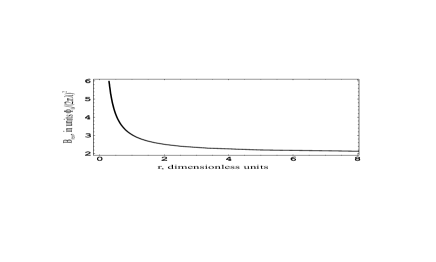
FIG. 1.: Critical field of 90^∘ VL reorientation as a function of parameter $r=-\lambda^{2}w_{6}/w_{4}$ (see Eq. (10))

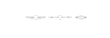
FIG. 2.: a) Diagrams of the order $1/N$, which vanish in our model. b) Diadrams of the order $1/N^{2}$ contributing to $w_{4}$. c) An example of complicated diagrams, which are of the order $1/N^{3}$ and were neglected.

REFERENCES

- [1] B. Keimer et al., Phys. Rev. Lett. 73, 3459 (1994).
- [2] T.M. Riseman et al., Nature 396 242 (1998).
- [3] M. R. Eskildsen et al., Phys. Rev. Lett. 78, 1968 (1997); M. Yethiraj et al., Phys. Rev. Lett. 78, 4849 (1997).
- [4] Y. De Wilde et al., Phys. Rev. Lett. 78, 4273 (1997).
- [5] V.G. Kogan et al., Phys. Rev. B 55, 8693 (1997).
- [6] D. McK. Paul et al., Phys. Rev. Lett. 80, 1517 (1998); A. B. Abrahamsen et al., Bulletin of the March Meeting of APS, Atlanta, 44, No.1, UC27.3; L. Vinnikov (unpublished).
- [7] V.G. Kogan et al., Phys. Rev. B, 54, 12386 (1996).
- [8] D. Chang et al, Phys. Rev. B 57, 7955 (1998); K. Park and D.A. Huse, Phys. Rev. B 58, 9427 (1998).
- [9] L. Civale et al, Phys. Rev. Lett. 83, 3920 (1999); V.G. Kogan et al Phys. Rev. B 60 (1999) 12577.
- [10] K. O. Cheon et al., Phys. Rev. B, 58, 6463 (1998); P. L. Gammel et al. Phys. Rev. Lett. 86, 4082 (1999).
- [11] M. R. Eskildsen et al., unpublished.
- [12] M. Franz, I. Affleck and M. H. S. Amin, Phys. Rev. Lett. 79 (1997) 1555.
- [13] A.L. Fetter and J.D. Walecka, Quantum theory of many-particle systems, Mc-Graw–Hill, Inc., 1971.
- [14] B.Rosenstein, B.J. Warr, and S.H. Park, Phys. Rep. 205, 59 (1991); G. Kotliar, Correlated Electron Systems, edited by V.J. Emery, World Scientific, Singapore, 1993.
- [15] In-Sang Yang et al., cond-mat/9910087.