Bouncing–ball tunneling in quantum dots

Abstract

We show that tunneling through quantum dots can be completely dominated by states quantized on stable bouncing–ball orbits. The fingerprints of bouncing–ball tunneling are sequences of Coulomb blockade peaks with strongly correlated peak height and asymmetric peak line shape. Our results are in agreement with the striking correlations of peak height and transmission phase found in recent interference experiments with quantum dots.

Transport experiments with semiconductor quantum dots yield important information on the energy levels and the wave functions of confined many–electron systems [2]. In the Coulomb blockade regime current can flow only if two different charge states of the quantum dot are tuned to have the same energy. This produces large nearly equally spaced conductance peaks as a function of the dot potential (tuned via electrostatic gates). At low temperatures, the magnitude of each conductance peak directly measures the magnitude of a single resonant wave function near the contacts to the leads. Some years ago, a statistical theory for the peak height distribution was developed [3] based on the assumption that the wave functions are completely uncorrelated and described by random matrix theory. Recent experiments [4, 5] found good agreement with the predicted distributions. At the same time, one of these experiments [5] reported large correlation between the heights of adjacent peaks. Much stronger correlations of both the peak height and the phase of the transmission amplitude through a quantum dot were observed in novel interference experiments [6, 7]. The correlations in these experiments comprised all Coulomb blockade peaks found in a gate voltage scan, yielding sequences of more than 10 correlated peaks.

Theoretical work [8] demonstrated that nonzero temperature can partially account for but not fully explain the peak correlations observed in Ref. [5]. More recently [9], it was shown that additional correlations can arise from short periodic orbits. Such orbits lead to deviations from random matrix predictions even for dots whose classical dynamics is completely chaotic. The predicted peak modulations [9] are of the type observed in Ref. [5], but can not account for the much stronger correlations in the interference experiments [6, 7]. Despite of considerable theoretical efforts [10, 11, 12] the origin of these correlations has not been understood. In particular, the most striking feature of the experiments [6, 7], that the correlations comprise all observed Coulomb peaks, has not been explained. We address this feature below.

We show that tunneling through quantum dots can be completely dominated by wave functions quantized on stable bouncing–ball orbits. Bouncing–ball tunneling (BBT) dominates the transport if (i) the leads are attached opposite to each other and (ii) if they are sufficiently wide providing near normal injection of electrons into the dot. Under the conditions (i) and (ii) the dot conductance exhibits sequences of strongly correlated Coulomb peaks. All peaks within a sequence are dominated by the same bouncing–ball mode. The unique fingerprint of BBT is a characteristic asymmetry of the peak line shape for the peaks in the tails of the sequences. This asymmetry is caused by the breaking of the particle–hole symmetry as the bouncing–ball state moves away from the Fermi energy. We find the asymmetry in the line shapes measured in Ref. [7], and suggest that the inspection of line shapes be used as a diagnostic for BBT in other experiments on quantum dots.

Our starting point is the transmission probability $T_{\rm ring}$ through an Aharonov–Bohm ring with a quantum dot embedded in one arm. We assume that the dot is in the Coulomb blockade regime. The tunnel barriers around the quantum dot suppress multiple reflections of electrons across the ring, and $T_{\rm ring}$ is given by [12]

$$T_{\rm ring}=\int dE\left(-{\partial f\over\partial E}\right)\left|t_{0}+t(E)\exp[2\pi i\Phi/\Phi_{0}]\right|^{2}.$$ (1)

Here, $\Phi$ is the magnetic flux through the ring, $\Phi_{0}$ is the flux quantum, and $t_{0}$, $t(E)$ are the transmission amplitudes through the free arm and the arm with the quantum dot, respectively ($t_{0}$ is assumed to be independent of injection energy). The ring is connected to two reservoirs labeled up (U) and down (D) occupied according to the Fermi distribution $f$. Below, we investigate the phase $\phi_{\rm QD}\equiv{\rm arg}\int dE(-\partial f/\partial E)t(E)$ and the transmission coefficient $T_{\rm QD}\equiv\int dE(-\partial f/\partial E)|t(E)|^{2}$. Both can be measured in quantum dot interference experiments [6, 7].

The transmission amplitude $t(E)$ is related to the retarded Green function $G_{pq}$ of the quantum dot,

$$t(E)=\sum_{pq}V_{p}^{U}V_{q}^{D}G_{pq}(E),$$ (2)

where $V_{p}^{l}$ is the matrix element for tunneling between level p in the dot and the reservoir $l=U,D$. For a weakly coupled dot the width of the level $p$ is given by $\Gamma_{p}=\Gamma_{p}^{U}+\Gamma_{p}^{D}$, where $\Gamma_{p}^{l}=|V_{p}^{l}|^{2}$ is the partial width for decay into the reservoir $l$. The matrix element is expressed [9] as

$$V_{p}^{l}=\left({\hbar^{2}\over m^{*}}\right)\left.\int ds\psi_{l}(s,z)\partial_{z}\psi_{p}^{*}(s,z)\right|_{z=0},$$ (3)

where the integration is performed along the edge between the potential barrier and the quantum dot ($\partial_{z}$ denotes the derivative normal to the barrier). The wave function $\psi_{p}$ corresponds to Dirichlet boundary conditions in the dot, while the barrier tunneling is fully included in the lead wave function $\psi_{l}$. The transverse potential in the tunneling region can be taken quadratic [9] yielding $\psi_{l}\sim c_{l}\exp[-(s-s_{l})^{2}/2a_{\rm eff}^{2}]$, where $s$ is the transverse coordinate, $s_{l}$ the center of the constriction and $a_{\rm eff}$ its effective width. We can restrict ourselves to the lowest transverse mode since higher modes are suppressed by the barrier penetration factor (included in $c_{l}$). The Gaussian form of the lead wave function is convenient but not crucial for the results presented below.

We obtain the dot wave functions $\psi_{p}$ for an effective potential which accounts for the dot confining potential and the interactions in the dot in a mean–field sense. We use a billiard approximation and model the dot by a hard–wall potential at the boundary, parameterized in polar coordinates by $R(\phi)=R_{0}[1+\epsilon\cos(2\phi)]$. The parameter $\epsilon$ measures the quadrupolar deformation out of circular shape. We use nonzero $\epsilon$ to mimic [13] the dots used in [6, 7]. As in the experiments, we assume that the leads are attached opposite to each other at the boundary points closest to the origin (the points with $\phi=\pm\pi/2$). In contrast to most studies of quantum dots which assume the dynamics in the dot to be either regular or fully chaotic, our boundary parameterization yields mixed classical motion. This is illustrated for $\epsilon=0.2$ in Fig. 2, showing chaotic motion in most of phase space except for two large islands associated with stable bouncing–ball motion between the contacts to the leads. We note that billiards of quadrupolar or similar shape have recently been used in studies of optical microresonators [14, 15].

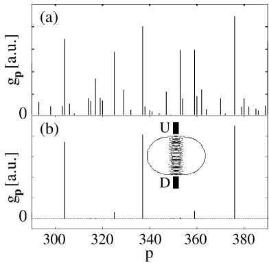
FIG. 1.: Coupling strength $g_{p}$ for a sequence of 100 states in the interval $290\leq p\leq 390$. Results are for a quantum dot with quadrupolar shape and deformation $\epsilon=0.2$. (a) Narrow leads: $ka_{\rm eff}=0.1$. (b) Wide leads: $ka_{\rm eff}=5.0$. Here $k=(2m^{*}E_{p})^{1/2}/\hbar$ is the wave number associated with the bouncing–ball state $p=337$. Inset: Real–space projection of the state $p=337$.

In Fig. 1 we show the coupling strength $g_{p}\equiv\Gamma_{p}^{U}\Gamma_{p}^{D}/(\Gamma_{p}^{U}+\Gamma_{p}^{D})$ over a sequence of 100 billiard states for two different values of $a_{\em eff}$. Note that $g_{p}$ is proportional to the conductance peak height $G_{p}=(e^{2}/h)(\pi/2kT)g_{p}$ measured in low temperature Coulomb blockade experiments [2]. We calculated $g_{p}$ from Eq. (3) using quantum dot wave functions obtained numerically with the boundary integral method [16]. For narrow leads the peak heights fluctuate with the level index $p$, occasionally one observes systematic peak modulations as reported in Ref. [9]. In striking contrast, the results for wide leads show a few isolated large peaks, separated by $15-25$ levels with much smaller peak height (not visible on the scale of Fig. 1(b)). All large peaks are associated with states quantized on stable bouncing–ball orbits. This is illustrated in the inset for the state $p=337$. The height of the small peaks not resolved in Fig. 1(b) is typically two or more orders of magnitude smaller than the maximum peak height. Such tiny peaks are difficult to resolve in standard Coulomb blockade experiments. The interference experiments [6, 7] face additional noise from the transmission through the free arm of the ring. For wide leads, interference experiments are therefore only sensitive to the strongly coupled bouncing–ball modes.

The crucial role of the transverse barrier width $a_{\em eff}$ can be understood from the following argument: Confinement in a lead of width $a_{\rm eff}$ yields the transverse momentum spread $\hbar/a_{\em eff}$ for electrons injected in the quantum dot. Wide leads therefore result in near normal injection and provide exceptionally strong coupling to the bouncing–ball states. To quantify this argument we express the partial width $\Gamma_{p}^{l}=|V_{p}^{l}|^{2}$ in terms of the Husimi function $H_{p}$. Recalling the Gaussian form of $\psi_{l}$ and using the arc length $s$ as integration variable in Eq. (3), we find

$$\Gamma_{p}^{l}=\left({|c_{l}|\hbar^{2}\over m^{*}}\right)^{2}H_{p}(s^{l},0),$$ (4)

where $H_{p}$ is calculated for the normal derivative of the wave function $\psi_{p}$. The Husimi function is evaluated at the phase space point ($s=s^{l},p_{s}=0)$ reflecting the position $s_{l}$ of the lead and zero transverse momentum. We note that the Husimi function can be written as an integral over the Wigner function, smoothed with Gaussians both in arc length and transverse momentum. Their width is given by $a_{\rm eff}/\sqrt{2}$ and $\hbar/\sqrt{2}a_{\rm eff}$, respectively. We express these widths in terms of the uncertainties $\Delta\phi$, $\Delta\sin\chi$ in polar angle $\phi$ and injection angle $\chi$, respectively ($\chi$ is the angle between the momentum of the injected electrons and the normal to the boundary). Using the relation $p_{s}=p\sin\chi$, we find $\Delta\phi\approx 0.7(ka_{\rm eff})/(kR_{0})$ and $\Delta\sin\chi\approx 0.7/(ka_{\rm eff})$, where $R_{0}$ is the average radius of the dot.

The phase space portrait of the dot with deformation $\epsilon=0.2$ is shown in Fig. 2 using $(\phi,\sin\chi)$ coordinates. Superimposed is the Husimi function of the bouncing–ball mode $p=337$ calculated for $ka_{\em eff}=5.0$ and $kR_{0}\approx 40$, corresponding to approximately $400$ electrons on the dot. The Husimi function attains maximum value at the phase space points $(\phi,\sin\chi)=\pm(\pi/2,0)$ representing normal injection from the leads.

In order to obtain the Husimi function and hence $\Gamma_{p}$ analytically, we must solve for the wave function $\psi_{p}$. For states localized on a chain of stable islands the calculation can be carried out using the semiclassical theory developed in Refs. [17, 15]. The result can be expressed in terms of the stable periodic orbit at the center of the island,

$$H_{p}(s,p_{s})= \sum_{\mu}{A_{\mu}\over\Delta s_{\mu}\Delta p_{\mu}}\exp\left[-\left(s-s_{\mu}\over\Delta s_{\mu}\right)^{2}\right]$$ (6)

$$\hskip 28.45274pt\times\exp\left[-\left(p_{s}-p_{\mu}\over\Delta p_{\mu}\right)^{2}\right],$$

where $s_{\mu}$ is the arc length and $p_{\mu}$ the transverse momentum at the bounce points $\mu$ of the periodic orbit. Moreover, $\Delta s_{\mu}=[a_{\rm eff}^{2}+l_{\mu}^{2}]^{1/2}$ and $\Delta p_{\mu}=[(\hbar/a_{\rm eff})^{2}+(\hbar/l_{\mu})^{2}]^{1/2}$ where $l_{\mu}=\sqrt{2\hbar|m_{12}^{\mu}|}|4-{\rm Tr}^{2}[M_{\mu}]|^{-1/4}$ is determined by the monodromy matrix $M_{\mu}\equiv(m_{ij}^{\mu})$. The amplitude $A_{\mu}$ depends only weakly on $a_{\rm eff}$. The result (6) allows us to express the width of island states in terms of the phase space distance of the underlying periodic orbit from the lead injection points. No comparable analytical result is known for states quantized in the chaotic sea. However, we find numerically that for wide leads the Husimi function of such states has exponentially small support near the injection points (see the inset of Fig. 2).

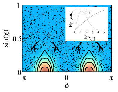
FIG. 2.: Husimi projection (color scale: red indicates high probability) of the bouncing–ball mode $p=337$ calculated for $ka_{\rm eff}=5.0$ and $\epsilon=0.2$. Superimposed is the Poincare surface of section of the classical phase space in $(\phi,\sin\chi)$ coordinates. Inset: $H_{p}(\phi=\pi/2,0)$ vs. $ka_{\rm eff}$ for the states $p=337$ (solid line) and $p=347$ (dashed line, enhanced by a factor $18$), the latter state is localized in the chaotic region of phase space.

We now turn to the calculation of the transmission coefficient $T_{\rm QD}$ and the phase $\phi_{\rm QD}$. We assume wide leads and temperature $kT<\Delta$. The calculation for the weak coupling limit $\Gamma_{p}\ll kT,\Delta$ is straightforward and can be done using the Green function derived in Ref. [12]; the results will be presented elsewhere [18]. Here, we address the regime of a more open dot as realized in the experiment [7]. This regime is characterized by $\Gamma_{\bar{p}}\sim\Delta$ where we identify $\bar{p}$ with the bouncing–ball state closest to the Fermi energy. All other states $p\neq\bar{p}$ in the vicinity of $E_{F}$ have a width $\Gamma_{p}\ll\Delta$. The Green function is found using the equations–of–motion method [19]. It is diagonal up to small off–diagonal corrections ${\cal O}(\sqrt{\Gamma_{p}\Gamma_{\bar{p}}}/\Delta)$, and given by

$$G_{\bar{p}\bar{p}}(E) = \sum_{N=0}^{\infty}{P_{N}\over E-[E_{\bar{p}}-eV_{g}+UN]+i\Gamma_{\bar{p}}/2}.$$ (7)

Here $N$ counts the total number of electrons in all dot levels except for the level $\bar{p}$, $P_{N}$ is the respective occupation probability, $E_{\bar{p}}$ is the single–particle energy of state $\bar{p}$, $V_{g}$ is the gate voltage, and $U=e^{2}/C$ is the charging energy. The transmission through the states $p\neq\bar{p}$ is negligible. Equation (7) is the generalization of the weak–coupling result [12] to the case of a single strongly conducting quantum state. The probability $P_{N}=Z^{-1}\exp[-\Omega(N)/kT]$ with $Z=\sum_{N}\exp[-\Omega(N)/kT]$ is related to the thermodynamic potential $\Omega(N)$ of the dot. To evaluate $P_{N}$ we replace $\Omega_{N}$ by $\Omega_{N}^{0}+[E_{\bar{p}}-eV_{g}+UN-E_{F}]\langle n_{\bar{p}}\rangle_{N}$, where $\Omega_{N}^{0}$ is calculated for the dot with level $\bar{p}$ excluded from the spectrum, and

$$\langle n_{\bar{p}}\rangle_{N}=-{1\over\pi}\int\!dE\,{\rm Im}{f(E)\over E-[E_{\bar{p}}-eV_{g}+UN]+i\Gamma_{\bar{p}}/2}$$ (8)

is the canonical occupation probability of level $\bar{p}$.

In Fig. 3 we show the transmission coefficient $T_{\rm QD}$ and the phase $\phi_{\rm QD}$ vs. gate voltage $V_{g}$ calculated for $kT=0.2\Delta$, $\Gamma_{\bar{p}}=1.5\Delta$ and $U=12\Delta$. All peaks shown result from transmission through the level $p=337$. The peaks have comparable height and similar phase in qualitative agreement with the experiments [6, 7]. The central peak has a Lorentzian shape of width $\Gamma_{\bar{p}}$. Note that the transmission peaks develop a peculiar asymmetry as the conducting level moves away from the Fermi energy: Each peak to the left and to the right of the central peak falls off more rapidly on the side facing the central peak. This pattern extends over the whole sequence and becomes more pronounced for the peaks in the tails. This asymmetry results from the breaking of the particle–hole symmetry in the transmission through the bouncing–ball state and is a unique fingerprint of BBT. Inspection of the data of the experiment [7] reveals the same asymmetry [20], providing strong evidence that the peak correlations in this experiment are due to BBT. We note that the number of correlated peaks in Fig. 3 is less than observed in experiment. The origin for this is addressed below. A detailed discussion of this issue and of the phase lapse between the peaks will be given in a future publication [18].

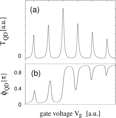
FIG. 3.: (a) Transmission coefficient $T_{\rm QD}$ and (b) phase $\phi_{\rm QD}$ as a function of gate voltage $V_{g}$ evaluated for $kT=0.2\Delta$, $\Gamma_{\bar{p}}=1.5\Delta$, and $U=12\Delta$. The peak asymmetry in (a) is a unique fingerprint of BBT.

We finally address the universality of the results presented above. The stability of bouncing–ball motion does not rely on the effective dot potential considered here. Similar stability if found for dots of other shapes [14, 15] as well as for smooth confining potentials [10]. We assumed that the dot shape does not change upon the addition of electrons. Some robustness of the shape has indeed been demonstrated in a recent experiment [21]. In general, however, variation of the gate voltage is expected [10, 22] to change the electrostatic potential and modify the shape of the dot. It was shown [10, 22] that shape deformations can enhance peak correlations by “pinning” conducting levels close to the Fermi energy. To study the effect of deformations, we varied the shape by a parameter linear in gate voltage $V_{g}$. Over a range of $V_{g}$ we observed the predicted enhancement of correlations and sequences of more than 10 correlated peaks. At the same time, the bouncing–ball modes changed very little with $V_{g}$ as substantial modification of the shortest stable modes typically requires a large change in potential.

In conclusion, we have demonstrated a new mechanism for transport through quantum dots in the Coulomb blockade regime. Current flows by tunneling through bouncing–ball modes. The fingerprints of bouncing–ball tunneling are sequences of correlated conductance peaks with asymmetric peak line shape. We find the peak asymmetries in recent Coulomb blockade interference experiments, providing strong evidence that the peak correlations in these experiments are caused by bouncing–ball tunneling.

We acknowledge helpful conversations with F. Haake and H. A. Weidenmüller. The work was supported by the Deutsche Forschungsgemeinschaft, DGAPA–UNAM, and CONACyT–Mexico.

REFERENCES

- [1]
- [2] L. P. Kouwenhoven et al., in Mesoscopic Electron Transport, edited by L. L. Sohn, L. P. Kouwenhoven, and G. Schön (Kluwer, Dordrecht, 1997).
- [3] R. A. Jalabert, A. D. Stone, and Y. Alhassid, Phys. Rev. Lett. 68, 3468 (1992).
- [4] A. M. Chang et al., Phys. Rev. Lett. 76, 1695 (1996).
- [5] J. A. Folk et al., Phys. Rev. Lett. 76, 1699 (1996).
- [6] A. Yacoby, M. Heiblum, D. Mahalu, and M. Shtrikmann, Phys. Rev. Lett. 74, 4047 (1995).
- [7] R. Schuster, E. Buks, M. Heiblum, D. Mahalu, V. Umansky, and H. Shtrikmann, Nature 385, 417 (1997).
- [8] Y. Alhassid, M. Gökçedaǧ, and A. D. Stone, Phys. Rev. B 58, R7524 (1998).
- [9] E. E. Narimanov, N. R. Cerruti, H. U. Baranger, and S. Tomsovic, Phys. Rev. Lett. 83, 2640 (1999).
- [10] G. Hackenbroich, W. D. Heiss, and H. A. Weidenmüller, Phys. Rev. Lett. 79, 127 (1997).
- [11] P. G. Silvestrov and Y. Imry, cond-mat/9903299.
- [12] R. Baltin and Y. Gefen, Phys. Rev. Lett. 83, 5094 (1999).
- [13] These dots were defined by surface gates of rectangular shape. The gates create a smooth dot shape in the electron gas below the surface.
- [14] J. U. Nöckel and A. D. Stone, Nature (London) 385, 47 (1997).
- [15] E. E. Narimanov, G. Hackenbroich, P. Jacquod, and A. D. Stone, Phys. Rev. Lett. 83, 4991 (1999).
- [16] M. Sieber and F. Steiner, Phys. Lett. 148A, 415 (1990).
- [17] E. E. Narimanov and A. D. Stone, Physica D 131, 220 (1999).
- [18] G. Hackenbroich and R. A. Mendez, unpublished.
- [19] Y. Meir, N. S. Wingreen, and P. A. Lee, Phys. Rev. Lett. 66, 3048 (1991).
- [20] The same type of peak asymmetry has been observed by J. Göres et al., cond-mat/9912419.
- [21] D. R. Stewart et al., Science 278, 1784 (1997).
- [22] R. O. Vallejos, C. H. Lewenkopf, and E. R. Mucciolo, Phys. Rev. Lett. 81, 677 (1998).