Nonlinear analysis of the shearing instability in granular gases

Abstract

It is known that a finite-size homogeneous granular fluid develops an hydrodynamic-like instability when dissipation crosses a threshold value. This instability is analyzed in terms of modified hydrodynamic equations: first, a source term is added to the energy equation which accounts for the energy dissipation at collisions and the phenomenological Fourier law is generalized according to previous results. Second, a rescaled time formalism is introduced that maps the homogeneous cooling state into a nonequilibrium steady state. A nonlinear stability analysis of the resulting equations is done which predicts the appearance of flow patterns. A stable modulation of density and temperature is produced that does not lead to clustering. Also a global decrease of the temperature is obtained, giving rise to a decrease of the collision frequency and dissipation rate. Good agreement with molecular dynamics simulations of inelastic hard disks is found for low dissipation.

I Introduction

The understanding of the dynamics of granular fluids is crucial for various industrial processes. This has led to many investigations where theory, experiments and simulations are used in order to construct a predictive theory [1, 2, 3, 4, 5, 6, 7, 8]. There is hope that for moderate densities and slightly dissipative grains, grain dynamics may be described on large scales by using fluid hydrodynamics with slight modifications.

One way to guess which changes to make in standard hydrodynamics is to use the tools developed by statistical mechanics in order to derive hydrodynamic equations. This is justified by the fact that a simple grain model, the inelastic hard sphere model, has been shown to reproduce most of the phenomena occuring in granular systems: in some sense, it has proven to contain the essential ingredients necessary to predict the peculiar physics observed [9, 10, 11, 12, 13, 14].

The scheme used in the study of nonequilibrium fluids can then be extended to granular fluids: “microscopic” simulations permit to compute the equation of state and values for transport coefficients which are then fed into the guessed macroscopic equations. Comparison between direct nonequilibrium simulations of microscopic and macroscopic models allows then to test the validity of the proposed macroscopic equations. This approach was used recently by two of us to investigate heat transport (heat being identified with the kinetic energy associated with the grains’ motion) and it has been shown that Fourier’s law has to be generalized with a density gradient term appearing in the expression for the heat flux [15].

In the Inelastic Hard Sphere model (IHS), grains are spherical hard particles with only translational degrees of freedom. The energy dissipation is included through a restitution coefficient $r$ lower than one. As for hard spheres, the collision is an instantaneous event and the grain velocities after a collision are given by

$${\bf v}_{1}^{\prime} = {\bf v}_{1}+\frac{1}{2}(1+r)\left[\widehat{\bf n}\cdot({\bf v}_{2}-{\bf v}_{1})\right]\widehat{\bf n}$$ (1)

$${\bf v}_{2}^{\prime} = {\bf v}_{2}-\frac{1}{2}(1+r)\left[\widehat{\bf n}\cdot({\bf v}_{2}-{\bf v}_{1})\right]\widehat{\bf n}$$ (2)

where $\widehat{\bf n}$ is the unit vector pointing from the center of particle 1 towards the center of particle 2. It is convenient to define the dissipation coefficient $q=(1-r)/2$ which vanishes when collisions are elastic. In what follows units are chosen such that the disk diameter $\sigma$ and the particles masses are set to one.

The IHS model, like the elastic hard sphere model, does not have an intrinsic energy scale. This means that two systems with the same initial configuration and with the particle velocities of one system being equal to those of the other multiplied by one scaling factor will follow the same trajectory but at different speeds. This lack of an intrinsic energy scale also implies a simple temperature dependence for all hydrodynamic quantities which may be found by simple dimensional analysis.

When a fluidized granular medium is let to evolve freely in a box with periodic boundary conditions, the energy decreases continuously in time and the system remains homogeneous. This non-steady state is called the Homogeneous Cooling State (HCS) and it is the reference state from which perturbations are studied: it is analogous to the thermodynamic equilibrium state for elastic systems [10, 16, 17]. In the IHS model this state is particularly simple and the energy decreases obeying the Haff’s law [18]

$$E(t)=\frac{E(0)}{\left(1+t/t_{0}\right)^{2}}$$ (3)

In order to avoid the cooling of the system, the simulations are made at constant energy: at every collision between the grains, the dissipated energy is redistributed by scaling all the velocities. This is equivalent to a time rescaling and can be treated as such in the equations for the continuous model. Using appropriate hydrodynamic equations, this homogeneous state is predicted to be unstable under certain conditions of density, system size and dissipativity [9, 10, 19, 16, 20, 21]. Considering the dissipativity coefficient q as a bifurcation parameter, while increasing q at constant density and number of grains, the system first develops an instability characterized by two counterflows, the shearing instability, and then either a clustering regime in which the density becomes inhomogeneous or a vortex state where many small vortices develop throughout the system.

For given values of total number of grains $N$ and number density $\rho=N/V$ the shearing instability appears when the dissipation coefficient is larger than a critical value. In the low density and large system limit,the critical value is given (in two dimensions) by [22]

$$\widehat{q}=\frac{\pi}{N\rho}$$ (4)

Note that in the thermodynamic limit the system is always unstable for any finite dissipation.

In this article we will study the shearing instability using a nonlinear hydrodynamic approach. In Sec. II we will develop a formalism that allows us to treat the HCS as a non equilibrium steady state, and we will present a stability analysis around the steady state. Next, in Sec. III we will present the nonlinear analysis of the instability, obtaining expressions for the hydrodynamic fields beyond the instability. It will also be shown that the presence of the instability modifies the collision rate and energy dissipation rate. Finally, in Sec. IV we compare the predictions of the continuous model with molecular dynamics simulations of inelastic hard disks. Conclusions are presented in Sec. V.

In what follows we will treat the two dimensional case, but the extension to three dimensions is direct.

II Rescaled time formalism

Consider a two dimensional system composed of $N$ grains interacting with the IHS model in a square box of size $L$ that has periodic boundary conditions in both directions. Units are chosen such that Boltmann’s constant and the particle masses are set to one. Granular temperature is defined analogously to the kinetic definition for classical fluids

$$T=\frac{1}{N}\sum_{i}\frac{1}{2}({\bf v}_{i}-{\bf v})^{2}$$ (5)

where ${\bf v}$ is the hydrodynamic velocity.

The shearing instability has been predicted by linear analysis of the hydrodynamic equations for the IHS. Also an analysis of the first stages of the nonlinear regime has been done in Ref. [23]. As we shall see, the relative simplicity of the model allows for a complete nonlinear analysis as well.

The hydrodynamic equations for the low-density IHS are similar to the usual hydrodynamic equations for fluids except that there is an energy sink term and the heat flux has contributions from the density gradient [22, 24, 16, 15]. The equations read

$$\frac{\partial\rho}{\partial t}+\nabla\cdot(\rho{\bf v})=0$$ (6)

$$\rho\left(\frac{\partial{\bf v}}{\partial t}+({\bf v}\cdot\nabla){\bf v}\right)=-\nabla\cdot I\!\!P$$ (7)

$$\rho\left(\frac{\partial T}{\partial t}+({\bf v}\cdot\nabla)T\right)=-\nabla\cdot{\bf J}-I\!\!P:\nabla{\bf v}-\omega$$ (8)

with the following constitutive equations

$$I\!\!P_{ij} = \rho T\delta_{ij}-\eta_{0}\sqrt{T}\left(\frac{\partial v_{i}}{\partial x_{j}}+\frac{\partial v_{j}}{\partial x_{i}}-(\nabla\cdot{\bf v})\delta_{ij}\right)$$ (9)

$${\bf J} = -k_{0}\sqrt{T}\nabla T-\mu_{0}\frac{T^{3/2}}{\rho}\nabla\rho$$ (10)

$$\omega = \omega_{0}\rho^{2}T^{3/2}$$ (11)

where $\eta_{0}$, $k_{0}$, $\mu_{0}$, and $\omega_{0}$ do not depend on density or temperature but on the dissipation coefficient $q$. In particular, $\omega_{0}$ and $\mu_{0}$ vanish with $q$.

The total energy dissipation rate can be computed from the hydrodynamic equations, obtaining

$$\frac{dE}{dt} = \frac{d}{dt}\int(\rho T+\rho v^{2}/2)\,dV$$ (12)

$$= -\int\omega\,dV$$ (13)

In the HCS, where density and temperature are homogeneous and there is no velocity field, the energy dissipation rate is

$$\frac{dE}{dt}=-V\omega_{0}\rho_{0}^{2}T^{3/2}\\$$ (14)

This continuous cooling down has the disadvantage that any perturbation analysis must be done with respect to this non-steady state. To overcome this difficulty we propose a differential time rescaling $ds=\gamma\,dt$ such that in this rescaled time, energy is conserved. The transformation corresponds to a continuous rescaling of all the particle velocities such that the kinetic energy remains constant. This rescaling does not, however, introduce new phenomena since as we have mentioned the IHS does not have an intrinsic time scale, and thus a time rescaling gives rise to the same phenomena viewed at different speed.

In order to keep the rescaled energy constant the appropriate value of $\gamma$ is given by

$$\gamma=\sqrt{\frac{E(t)}{E(0)}}$$ (15)

The rescaled time hydrodynamic fields transform as

$${\bf v} = \gamma\widetilde{{\bf v}}$$ (16)

$$T = \gamma^{2}\widetilde{T}$$ (17)

$$I\!\!P_{ij} = \gamma^{2}\widetilde{I\!\!P_{ij}}$$ (18)

$${\bf J} = \gamma^{3}\widetilde{{\bf J}}$$ (19)

$$\omega = \gamma^{3}\widetilde{\omega}$$ (20)

where the tilde denotes the rescaled variable.

Due to the non-constant character of the time rescaling, extra source terms appear in the hydrodynamic equations, which can be simplified using the relation

$$\frac{1}{\gamma}\frac{d\gamma}{ds}=-\frac{1}{2E(0)}\int\widetilde{\omega}\,dV$$ (21)

Suppressing the tildes everywhere, the equations now read:

$$\frac{\partial\rho}{\partial s}+\nabla\cdot(\rho{\bf v})=0$$ (22)

$$\rho\left(\frac{\partial{\bf v}}{\partial s}+({\bf v}\cdot\nabla){\bf v}\right)=-\nabla\cdot I\!\!P+\frac{\rho{\bf v}}{2E(0)}\int\omega\,dV$$ (23)

$$\rho\left(\frac{\partial T}{\partial s}+({\bf v}\cdot\nabla)T\right)=-\nabla\cdot{\bf J}-I\!\!P:\nabla{\bf v}-\omega+\frac{\rho T}{E(0)}\int\omega\,dV$$ (24)

Note that the constitutive relations (9) remain unchanged under time rescaling.

In the rescaled time, the HCS reduces to a non-equilibrium steady state with a continuous energy supply that compensates the energy dissipation. As there is no energy scale, we fix the reference temperature to be one, so that $E(0)=N$. The HCS is then characterized by $\{\rho=\rho_{H},\,T=1,\,{\bf v}=0\}$. To study the stability of this state, we first introduced the change of variables:

$$\rho = \rho_{H}+\delta\rho$$ (25)

$${\bf v} = \delta{\bf v}$$ (26)

$$T = 1+\delta T$$ (27)

Taking the (discrete) Fourier transform of the linearized hydrodynamic equations around HCS, it is easy to check that the transverse velocity perturbation decouples from the rest and satisfies the equation

$$\rho_{H}\frac{\partial\delta{\bf v}_{k_{\perp}}}{\partial s}=\lambda_{k}\delta{\bf v}_{k_{\perp}}$$ (28)

with

$$\lambda_{k}\equiv-\frac{4k^{2}\pi^{2}}{L^{2}}\eta_{0}+\frac{\rho_{H}^{2}\omega_{0}}{2}\,\,\,\,;\,\,\,\,\{k_{x},k_{y}\}\,=\,0,\pm 1,\,\pm 2,\,\dots$$ (29)

For small values of $\omega_{0}$ (proportional to the dissipation) $\lambda_{k}<0$, so that the perturbations $\delta{\bf v}_{k_{\perp}}$ decay exponentially (the case $k=0$ should not be taken into account since the center of mass velocity is strictly zero). But there exists a critical value of $\omega_{0}$ for which $\lambda_{k}$ vanishes, thus indicating the stability limit of the corresponding mode. The first modes to become unstable correspond to $|{\bf k}|=1$ (i.e, $k_{x}=\pm 1,\,k_{y}=0$ and $k_{x}=0,\,k_{y}=\pm 1$). The instability threshold for $\omega_{0}$ is then given by

$$\widehat{\omega}_{0}=\frac{8\pi^{2}\eta_{0}}{\rho_{H}^{2}L^{2}}$$ (30)

The stability for the other modes has been studied previously [16]. In this last reference, it was shown that for, low dissipation, the first instability that arises is indeed the transverse velocity instability.

The origin of the instability can be understood also in terms of the real time hydrodynamics. In fact, the relaxation of the transverse hydrodynamic velocity is basically due to the viscous diffusion, which depends on the system size, whereas the cooling process is governed by local dissipative collisions. There exists therefore a system length beyond which the dissipation of thermal energy is faster that the relaxation of the transverse hydrodynamic velocity. The latter will then increase, when observed on the scale of thermal motion, thus producing the shearing pattern.

III Nonlinear analysis of the instability

In this section we propose to work out the explicit form of the velocity field beyond the instability. The calculations are tedious and quite lengthy, so that, here, we only describe explicitely the basic steps. We start by taking the Fourier transform of the full nonlinear hydrodynamic equations, obtaining a set of coupled nonlinear equations for the modes { $\delta\rho_{k},\delta T_{k},\delta{\bf v}_{k_{\parallel}},\delta{\bf v}_{k_{\perp}}$ }, where $\delta{\bf v}_{k_{\parallel}}$ represents the longitudinal component of the velocity field. Close to the instability ($\omega_{0}\approx\widehat{\omega}_{0}$, $|{\bf k}|=1$), the modes $\delta{\bf v}_{1_{\perp}}$ exhibit a critical slowing down since $\lambda_{1}\approx 0$, whereas the other hydrodynamic modes decay exponentially (cfr. ref. [16]). On this slow time scale, i.e. $s\approx O(\lambda_{1}^{-1})$, the “fast” modes {$\delta\rho_{k};\delta T_{k};\delta{\bf v}_{k_{\parallel}};\delta{\bf v}_{k_{\perp}},k\neq 1$} can be considered as stationary, their time dependence arising mainly through $\delta{\bf v}_{1_{\perp}}$. Setting the time derivatives of these fast modes to zero one can express them in terms of the slow modes $\delta{\bf v}_{1_{\perp}}$. If now one inserts the so-obtained expressions into the evolution equation for the slow modes, one gets a set of closed nonlinear equations for $\delta{\bf v}_{1_{\perp}}$ (adiabatic elimination [25, 26]), usually referred to as normal form or amplitude equations [G. Nicolis, Introduction to Nonlinear Science, Cambridge University Press (1995) ]. Note that such a calculation is only possible close to the instability threshold, where the amplitude of $\delta{\bf v}_{1_{\perp}}$ approaches zero as $\omega\rightarrow\widehat{\omega}_{0}$. On the other hand, in this limit the only Fourier modes that will have large amplitudes are the transverse velocity modes with wavevector equal to $\pm\,2\pi/L$ (i.e. $|{\bf k}|=1$). There are four such modes:

$$\delta{\bf v}_{k_{\perp}}=\left\{\begin{array}[]{ll}A_{1}&{\bf k}=(1,0)\\ A_{1}^{*}&{\bf k}=(-1,0)\\ A_{2}&{\bf k}=(0,1)\\ A_{2}^{*}&{\bf k}=(0,-1)\\ \end{array}\right.$$ (31)

After some tedious algebra, one finds

$$\rho_{H}\frac{dA_{1}}{ds} = \lambda_{1}A_{1}-4\pi^{2}L^{-2}\eta_{0}\left(C_{1}\left|A_{1}\right|^{2}+C_{2}\left|A_{2}\right|^{2}\right)A_{1}$$ (32)

$$\rho_{H}\frac{dA_{2}}{ds} = \lambda_{1}A_{2}-4\pi^{2}L^{-2}\eta_{0}\left(C_{1}\left|A_{2}\right|^{2}+C_{2}\left|A_{1}\right|^{2}\right)A_{2}$$ (33)

where

$$C_{1} = \frac{8(k_{0}-\mu_{0})-3\eta_{0}}{8(k_{0}-\mu_{0})-2\eta_{0}}$$ (34)

$$C_{2} = \frac{2(k_{0}-\mu_{0})+\eta_{0}}{2(k_{0}-\mu_{0})-\eta_{0}}$$ (35)

The amplitude equations (32) and (33) admit three different stationary solutions:

$$(a)\hskip 8.5359pt A_{1}=0,\hskip 14.22636ptA_{2}=0$$ (36)

$$(b)\hskip 8.5359pt \left|A_{1}\right|=\widehat{A},\hskip 14.22636ptA_{2}=0$$ (38)

$$A_{1}=0,\hskip 14.22636pt\left|A_{2}\right|=\widehat{A}$$

$$(c)\hskip 8.5359pt \left|A_{1}\right|=\left|A_{2}\right|=\widehat{A}\,\sqrt{\frac{C_{1}}{C_{1}+C_{2}}}$$ (39)

where we have set

$$\widehat{A}=\frac{L}{2\pi}\,\sqrt{\frac{\lambda_{1}}{\eta_{0}C_{1}}}$$ (40)

Note that the phases of the above stationary solutions are arbitrary (recall that $A_{1}$ and $A_{-1}$ are complex conjugate).

The trivial solution (a) corresponds to a motionless fluid, whereas the solutions (b) are shearing states with the corresponding fluxes oriented either in the $y$ or $x$ direction. The mixed mode solution (c) represents a vortex state with two counter-rotating vortices in the box.

Below the critical point ($\lambda_{1}<0$), the trivial solution (a) is the only stable one. As we cross the critical point this solution becomes unstable. A linear stability analysis of the Eqs. 33 shows that the shearing states are stable provided

$$\frac{C_{2}}{C_{1}}>1$$ (41)

while the mixed mode solution is unstable. Satisfying Eq.41 depends on the values of the transport coefficients. For small dissipativity it is always fulfilled, provided the number density remains relatively low. In fact, a mixed mode state has been observed recently in a highly dense system [10].

The occurence of either shearing states depends on the initial state. In a statistical sense, they are equally probable. For example, in the case that the system chooses the solution {$A_{1}=\widehat{A}$, $A_{2}=0$}, the velocity field reads

$${\bf v}=2\widehat{A}\cos(2\pi x/L)\,\widehat{\bf y}$$ (42)

where $\widehat{\bf y}$ represents the unit vector in $Y$ direction. The temperature and density perturbations are then given by

$$\delta T = -(\widehat{A})^{2}\left[1+(1-C_{1})\cos(4\pi x/L)\right]$$ (43)

$$\delta\rho = \rho_{H}(\widehat{A})^{2}(1-C_{1})\cos(4\pi x/L)$$ (44)

The instability of the transverse velocity field thus gives rise to modifications of the temperature and density fields. The temperature decreases globally, since part of the energy is taken by the convective motion. Moreover, because of the viscous heating, the temperature profile exhibits a spatial modulation, i.e. it is higher where the viscous heating is higher. The density profile also shows a spatial modulation that keeps the pressure homogeneous (recall that for a two dimensional low density gas, $\delta p\approx\rho_{h}\delta T+\delta\rho$, in system units). This modulation of the density, that was first observed by Goldhirsh and Zanetti [9] (Fig. 2 of their article) in the study of the clustering instability, is stable and does not lead to clustering.

Using the above expressions for the hydrodynamic fields, the energy density profile reads

$$e=\rho_{H}\left(1+\widehat{A}^{2}\cos(4\pi x/L)\right)$$ (45)

Assuming the molecular chaos hypothesis, the mean collision rate, $\overline{\nu}$, and dissipation rate, $\overline{\omega}$, can be computed as well:

$$\overline{\nu} = \frac{2\sqrt{\pi}}{V\rho_{H}}\int\rho^{2}\sqrt{T}\,dV\,\,=\,\,\nu_{0}\rho_{H}\left(1-\frac{\widehat{A}^{2}}{2}\right)$$ (46)

$$\overline{\omega} = \frac{1}{V}\int\omega\,dV\,\,=\,\,\omega_{0}\rho_{H}^{2}\left(1-\frac{3\widehat{A}^{2}}{2}\right)$$ (47)

These relations show that the global decrease of the temperature leads to corresponding decreases of the collision frequency and dissipation rate.

It is important to note that the origin of the nonlinear coupling of slow modes lies in the viscous heating term and the state-dependence of the transport coefficients, and not in the usual convective derivatives ($({\bf v}\cdot\nabla){\bf v}$). In fact, as we have shown above, the shearing state produces a variation in the density and temperature fields that modify locally the value of the transport coefficients. This effect, which is negligible in classical fluids, can become very important in granular fluids, mainly because of the the lack of scale separation of the kinetic and hydrodynamic regimes. Contrary to normal fluids, here, the convective energy is comparable to the thermal energy. In fact, as will be shown in the MD simulations, in a well developed shearing state up to half of the total kinetic energy corresponds to the convective motion. The microscopic source of this phenomenon lies in the fact that only the relative energy is dissipated in binary collisions, i.e. the center of mass energy is conserved. In other words, the thermal energy is dissipated but the convective one is conserved. This asymmetry in the energy dissipation mechanism is at the very origin of the shearing instability.

IV Molecular dynamics simulations

For the molecular dynamic simulations we have considered a system made of $N\!=\!10000$ hard disks with a global number density $\rho_{H}\!=\!0.005$. Inelastic collision rules are adopted, with a dissipativity varying from $q\!=\!0.0$ to $q\!=\!0.12$. The boundary conditions are periodic in all directions. A spatially homogeneous initial condition is adopted, with velocities sorted from an equilibrium (zero mean velocity) Maxwellian distribution. We note that the density is low enough so that the system remains within the low-density regime.

The simulations have been performed in the rescaled time. Computationally, this is achieved by doing a normal IHS simulation (event driven molecular dynamics [27]), but at each collision the value of the kinetic energy is updated according to the energy dissipated. The instantaneous value of $\gamma$ is computed from the kinetic energy, allowing to evaluate all the rescaled quantities. Note that the $s$-time can be integrated in the simulation because $\gamma$ is a piecewise constant function, thus allowing to make periodic measurements in the system. Finally, to avoid roundoff errors, a real velocity rescaling is performed whenever the kinetic energy decreases by a given amount (typically $10^{-7}$ of the initial value).

In each simulation, the collision frequency and temperature dissipation rate are computed with respect to the $s$-time, after the system has reached a stationary regime. In Fig. 1, the collision frequency and the temperature dissipation rate are presented as a function of the dissipation coefficient $q$. As expected, the shearing instability is associated with an abrupt decrease of these functions. It must be noted that the decreasing of the collision frequency is more that $30\%$, which corresponds to a global decrease of the temperature of more than $50\%$. This means that when the shearing is fully developed, about half the total kinetic energy is taken by the macroscopic motion. This phenomenon is typical of granular media and has no counterpart in classical fluids.

To measure the critical point, $q_{0}$, we fit the collision frequency according to the following piecewise function

$$\overline{\nu}=\left\{\begin{array}[]{ll}a_{0}&q\leq q_{0}\\ a_{0}+a_{1}(q-q_{0})+a_{2}(q-q_{0})^{2}&q>q_{0}\end{array}\right.$$ (48)

obtaining

$$q_{0} = 0.0686$$ (49)

$$a_{0} = 0.0178$$ (50)

$$a_{1} = -0.167$$ (51)

$$a_{2} = 1.03$$ (52)

Similarly, the dissipation rate is fitted according to

$$\overline{\omega}=\left\{\begin{array}[]{ll}b_{0}q&q\leq q_{0}\\ b_{0}q+b_{1}(q-q_{0})q+b_{2}(q-q_{0})^{2}q&q>q_{0}\end{array}\right.$$ (53)

Using $q_{0}=0.0686$, one finds

$$b_{0} = 0.000166$$ (54)

$$b_{1} = -0.00466$$ (55)

$$b_{2} = 0.0546$$ (56)

To compare these results with our theoretical predictions we need the explicit form of the transport coefficients, up to critical dissipativity. Unfortunately, there are no known expressions for them in the case the $2d$ IHS model in the low-density regime. However, as the critical dissipativity is small we can use the the quasielastic approximation for the transport coefficients (that is, taking the first non-trivial order in $q$) [28, 22]

$$\omega_{0} = 4\sqrt{\pi}q$$ (57)

$$\eta_{0} = \frac{1}{2\sqrt{\pi}}$$ (58)

$$k_{0} = 2/\sqrt{\pi}$$ (59)

$$\mu_{0} = 0$$ (60)

The critical dissipativity and the amplitude of the shearing state are given by

$$\widehat{q} = \frac{\pi}{\rho_{H}^{2}L^{2}}$$ (61)

$$\widehat{A} = \rho_{H}L\sqrt{\frac{30}{29\pi}\delta q}$$ (62)

$$= \sqrt{\frac{30}{29}\frac{\delta q}{\widehat{q}}}$$ (63)

For the presented simulation, the predicted critical dissipativity is

$$\widehat{q}=0.0628$$ (64)

which shows a discrepancy of $8\%$ with the observed value. This difference is consistent with the adopted approximations.

The predicted values for $a_{0}$, $a_{1}$, $b_{0}$, $b_{1}$ (cfr. Eqs. 46, 47, 61, and 63) are

$$a_{0} = 0.0177$$ (65)

$$a_{1} = -0.146$$ (66)

$$b_{0} = 0.000177$$ (67)

$$b_{1} = -0.00438$$ (68)

which are also consistent with the adopted approximations.

Since the system is periodic, the developed convective pattern can diffuse in the direction perpendicular to the flow (the phases of the complex amplitudes $A_{i}$ are arbitrary due to Galilean invariance). As a result, the average hydrodynamic fields remain vanishingly small, mainly because of “destructive” interference. To overcome this difficulty we have performed another series of simulations, keeping periodic boundary conditions in the vertical direction, while introducing a pair of stress-free and perfectly insulating parallel walls in the horizontal direction (in a collision with a wall the tangential velocity is conserved whereas the normal one is inverted). As a consequence, the total vertical momentum is conserved, which will be simply set to zero initially.

The nonlinear analysis for this case is similar to the periodic one, except that, here, the direction of the flow pattern remains always parrallel to the walls. Furthermore, the unstable wavevector is now $k=\pi/L$, because of to the fixed boundary conditions. As a result all the previous predictions remain valid, except that everywhere $L$ must be replaced by $2L$.

We have used the very same number of particles and density for this series of simulations, but, of course, the different boundary conditions produce a new critical dissipativity. Performing the same analysis as before, the measured critical point and fit parameters turn out to be

$$q_{0} = 0.0163$$ (69)

$$a_{0} = 0.0178$$ (70)

$$a_{1} = -0.562$$ (71)

$$a_{2} = 8.93$$ (72)

$$b_{0} = 0.000175$$ (73)

$$b_{1} = -0.0179$$ (74)

$$b_{2} = 1.06$$ (75)

while the predicted ones are

$$\widehat{q} = 0.0157$$ (76)

$$a_{0} = 0.0177$$ (77)

$$a_{1} = -0.583$$ (78)

$$b_{0} = 0.000177$$ (79)

$$b_{1} = -0.0175$$ (80)

Eqs. 42, 44, and 45, once $L$ is replaced by $2L$, indicate that the perturbation of the transverse momentum density (${\bf j}=\rho{\bf v}$) has a wavevector equal to $k_{x}=\pi/L$, while the density and energy density have wavevectors $k_{x}=2\pi/L$. In the simulations we computed the amplitudes of these Fourier modes using the microscopic definitions for the particle, momentum, and energy densities. Figs. 2, 3, and 4 show the predicted and computed Fourier modes amplitudes. The predictions are in good agreement with the simulations in the neighborhood of the critical point, showing that not only the average quantities like the collision frequency are well predicted, but also the whole hydrodynamic picture is correct.

V Conclusions

Taking advantage of the lack of energy scale in the IHS model, a rescaled time formalism was introduced that allows us to study the homogeneous cooling state as a nonequilibrium steady state. Using a hydrodynamic description for granular media written with a rescaled time variable, the shearing instability has been studied in the nonlinear regime. It has been shown that the shearing state is the stable solution and its amplitude has been computed. The appearance of the velocity field produces that part of the kinetic energy goes from the kinetic to the hydrodynamic scale. In usual fluids this redistribution of the energy is negligible, but in granular fluids it can represent an important fraction of the total energy. This phenomenon is a manifestation of a global property of granular fluids: there is not in general a clear separation between the kinetic and the hydrodynamic regimes. This could lead to put into question the validity of a hydrodynamic description. Nevertheless, at small values of the dissipativity coefficient, predictions based on the nonlinear hydrodynamic equations are in excellent agreement with molecular dynamics simulations. Both the value of the critical dissipativity and the behavior after the instability has developed are well predicted. This is a remarkable result which shows again how robust the hydrodynamic fluid equations are when they are tested at time and length scales where their validity could be questioned.

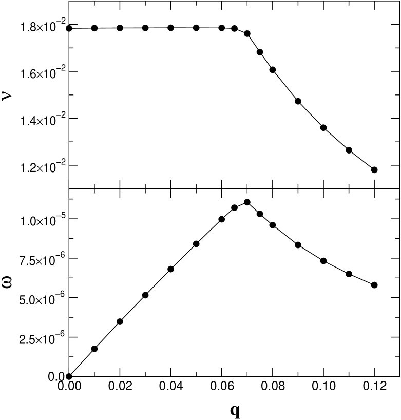
FIG. 1.: Mean collision frequency $\overline{\nu}$ and dissipation rate $\overline{\omega}$ as a function of the dissipativity $q$ obtained in molecular dynamics simulations with $N=10000$ particles and density $n=0.005$. The lines are drawn for easier reading of the graphs.

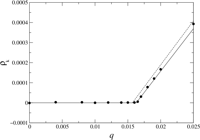
FIG. 2.: Amplitude of the $k_{x}=2\pi/L$ cosine component of the density field as a function of the dissipativity $q$. The dots are the results of molecular dynamics simulations, the dashed line is the full nonlinear theory prediction, and the solid line is the nonlinear theory prediction where the critical point is taken from the fit. The simulations were done in a channel with $N=10000$ particles and density $n=0.005$.

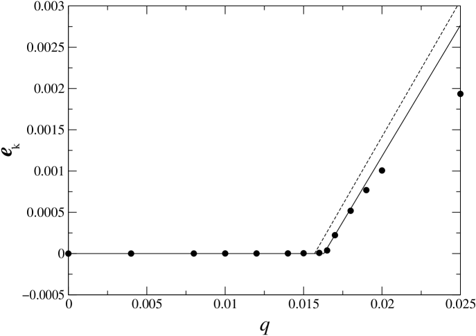
FIG. 3.: Amplitude of the $k_{x}=2\pi/L$ cosine component of the energy density field as a function of the dissipativity $q$. Graph symbols and simulation parameters are explained in Fig. 2.

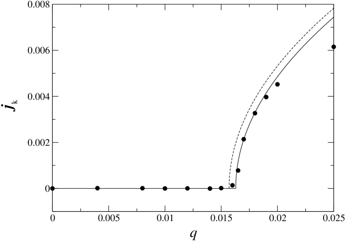
FIG. 4.: Amplitude of the $k_{x}=\pi/L$ cosine component of the momentum density field as a function of the dissipativity $q$. Graph symbols and simulation parameters are explained in Fig. 2.

REFERENCES

- [1] C. S. Campbell, Annu. Rev. Fluid Mech. 22, 57 (1990).
- [2] H. M. Jaeger and S. R. Nagel, Science 255, 1523 (1992).
- [3] F. Melo, P. B. Umbanhowar, and H. L. Swinney, Phys. Rev. Lett. 72, 172 (1994).
- [4] P. B. Umbanhowar, F. Melo, and H. L. Swinney, Nature 382, 793 (1996).
- [5] H. M. Jaeger, S. R. Nagel, and R. P. Behringer, Physics Today 49, 32 (1996).
- [6] J. S. Olafsen and J. S. Urbach, Phys. Rev. Lett. 81, 4369 (1998).
- [7] E. Falcon, R. Wunenburger, P. Évesque, and S. Fauve, Phys. Rev. Lett. (to appear) (1999).
- [8] R. Wildman, J. Huntley, and J.-P. Hansen, Phys. Rev. E 50, 7066 (1999).
- [9] I. Goldhirsch and G. Zanetti, Phys. Rev. Lett. 70, 1619 (1993).
- [10] S. McNamara and W. R. Young, Phys. Rev. E 53, 5089 (1996).
- [11] M. Müller, S. Luding, and H. J. Herrmann, in Friction, Arching and Contact Dynamics, edited by D. E. Wolf and P. Grassberger (World Scientific, Singapore, 1997).
- [12] P. Zamankhan, A. Mazouchi, and P. Sarkomaa, Appl. Phys. Lett. 71, 26 (1997).
- [13] E. L. Grossman, T. Zhou, and E. Ben-Naim, Phys. Rev. E 55, 4200 (1997).
- [14] D. C. Rapaport, Physica A 249, 232 (1998).
- [15] R. Soto, M. Mareschal, and D. Risso, Phys. Rev. Lett. 83, 5003 (1999).
- [16] J. J. Brey, F. Moreno, and J. W. Dufty, Phys. Rev. E 54, 445 (1996).
- [17] T. P. C. van Noije and M. H. Ernst, Granular Matter 1, 57 (1998).
- [18] P. K. Haff, J. Fluid Mech. 134, 401 (1983).
- [19] J. J. Brey, M. J. Ruiz-Montero, and D. Cubero, Phys. Rev. E 54, 3664 (1996).
- [20] T. P. C. van Noije, M. H. Ernst, E. Trizac, and I. Pagonabarraga, Phys. Rev. E 59, 4326 (1999).
- [21] P. Deltour and J.-L. Barrat, J. Phys. I France 7, 137 (1997).
- [22] J. T. Jenkins and M. W. Richman, Arch. Rat. Mech. 87, 355 (1985).
- [23] J. J. Brey, M. Ruiz-Montero, and D. Cubero, Phys. Rev. E 60, 3150 (1999).
- [24] J. T. Jenkins and S. B. Savage, J. Fluid Mech. 130, 187 (1983).
- [25] H. Haken, Springer Ser. Synergetics, Vol. 1 (Springer, Berlin, 1983).
- [26] G. Nicolis, Introduction to Nonlinear Science (Cambridge University Press, Cambridge, 1995).
- [27] M. Marín, D. Risso, and P. Cordero, J. Comput. Phys. 109, 306 (1993).
- [28] J. V. Sengers, Phys. Fluids 9, 1333 (1966).