On depolarisation level shift in spherical QD

Abstract

A giant level shift, resulted from the interaction of an electron in a spherical quantum dot with zero–point oscillations of confined modes of the electric field, is divulged. The energy correction depends on the dot radius. This size scaling of the depolarisation effect is computed semiclassically. A change of the optical properties of the matrix surrounding the dot provides a method to study the shift experimentally.

I Introduction

A complete quantum dot (QD) theory, taking into account all the sophisticated physics of the object, is still a challenge for a theorist. The main reason is that the scale of the calculation is much larger than atomic one (that complicates ab initio techniques). The same time the number of particles is small to use solid state approximations in full extent. For example, an one–electron picture of a quantum confinement potential, arising from the conduction band discontinuity on the QD boundary, does not always yield accurate electron levels.

In the paper we put forward a model to inspect the electrodynamical correction to the one–electron energy in a spherical QD. It was shown[1] that the similar correction occurs to be significant for a ”natural quantum dot” C₆₀. A depolarisation level shift due to the interaction with an electromagnetic field is not negligible, as it might be thought, when taking into account localized electromagnetic modes. We present the scaling analysis of some different mechanisms for the level shift (LS) and propose a possible experimental manifestation of the depolarisation effect.

In order to appraise the LS a simple spherical QD model in frame of an effective mass approximation was applied. How is our result sensitive to the model used? The size scaling of the depolarisation shift preserves, being dependent mainly on a corresponding density of states of the field, while the prefactor might be smaller within other approach, though it is not easy to evaluate explicitly.

The group of full rotations, SO(3), was chosen to label the one–electron states. It is possible to perform an analytic quantum–mechanical calculation of the RPA response within the spherical model[2]. The massive peak of a collective excitation is known to show up in the spectrum, resulting from the fast coherent oscillation of the total electron density of the valence states. Thus, within our model the electron–electron interaction is dealt with selfconsistently. Of course, the number of valence electrons involved in the collective motion has not to be small. It is believed to fulfill for the typical QD possessing some hundreds of atoms and even more.

A surface charge density oscillation can be thought as a confined electric field mode or a multipole surface plasmon. We will reflect on the shift of the electron level in the field of zero–point oscillations of the modes connected with the QD, which depolarisation effect is billion times stronger than of the free field zero–point oscillations, so a name ”giant LS” is admitted.

The classical description of the electromagnetic surface modes, via the dielectric function of the matrix and QD material, gives the true plasmon state frequencies and will be used below. Once more, the final result does not depend too much on the computation approach. Our model sketches out the (many–body) depolarisation semiclassically, avoiding a lot of the routine computational intricacy.

The paper proceeds as follows: the brief model description is next to the introduction. Then, the model will be applied to a 3D–plasmon as well as a free field mode, that will explain the calculation technique. However, the LSs from these modes are too small to have an experimental importance. Section IV deals with the confined modes those result in much larger depolarisation shift. The numerical estimations and the scaling properties of the LS will be given in respect to a possible experiment. A brief summary will follow. The calculation of the QD confined mode frequencies is allocated in Appendix.

II Semiclassical theory for energy level shift

We have considered semiclassically the LS for an arbitrary shell object in [3]. The method follows the one proposed by Migdal[4] to calculate the Lamb shift for a hydrogen–like atom. The frequency of the zero–point oscillations of the external field is much higher than the inverse period of the electron orbit $\omega_{p}\gg\pi/\tau$. Therefore, the adiabatic approximation has to be used and one divides the fast (field) and slow (electron) variables. An electron is subjected to short fast deflections from its original orbit in the high–frequency field of the electromagnetic wave of the zero–point oscillation. Then the energy shift is given by the second order perturbation theory as

$$\delta E=\left<H(r+\delta)-H(r)\right>=\left<\nabla H\cdot\vec{\delta}+\frac{1}{2}\nabla^{2}H\;\vec{\delta}\cdot\vec{\delta}+\ldots\right>,$$ (1)

where $H(r)$ is the unperturbed Hamiltonian and $H(r+\delta)$ is the Hamiltonian with account for the random electron deflection $\delta$. The angle brackets represent the quantum mechanical average over the fast variables of the field (or, the same, over the random electron deflections). The perturbed Hamiltonian is expanded in series on the $\delta$ and a first nonzero contribution is taken.

The simplest QD Hamiltonian is considered to have only the rotational correction which is given by:

$$\delta H=\frac{{\hat{L}}^{2}}{2mR^{2}}\left(-2\frac{\delta}{R}+3\frac{\delta^{2}}{R^{2}}+\ldots\right),$$ (2)

where $R$ is about the spherical QD radius; $m$ is the electron mass which is supposed to be constant within the dot; $\hat{L}$ is the angular momentum operator. On the averaging, the first–order term disappears. So far the LS dependence on the QD size includes $R^{-4}$ factor besides some power hidden in the mean square deflection $\overline{\delta^{2}}$. The strength of the electrodynamical interaction changes with this quantity almost exactly. We will show that the dependence of $\overline{\delta^{2}}$ in $R$ is different for different electric modes (confined and free field). The giant deflection is representative for the giant LS and, therefore, the function $\overline{\delta^{2}}(R)$ will be studied specifically.

III Bulk plasmon contribution to LS

First we consider the bulk 3D–plasmon modes that could shift the electron level. Nearly self–evidently the bulk plasmon shift is negligible. The mean square deflection, caused by the 3D mode (which is not confined at all), decreases with the QD size too rapidly. The small factor, contained in the 3D LS, comes essentially from the expression for $\overline{\delta^{2}}$ which scales as $1/N$, where $N$ is the number of atoms in the QD. It will be explained in this section.

Within the semiclassical approach, the deflection of the electron can be computed with the use of the Newton law:

$$m\partial_{t}^{2}\delta=e{\cal E},$$ (3)

here $e$ is the electron charge, ${\cal E}$ is the field strength due to the zero–point oscillation of some mode, $m$ is the electron effective mass. The square of the deflection $\overline{\delta^{2}}=e^{2}/(2m)^{2}\int d^{D}k\;\overline{{\cal E}_{k}^{2}}/\omega_{k}^{4}$ is proportional to the mean square of the electric field strength. The dimension of the field, $D$, equals 3. The field strength, in turn, can be rewritten as the zero–point oscillation frequency $\overline{{\cal E}_{k}^{2}}=2\pi\hbar\omega_{k}$ through the quantized field normalisation.

The scale of the energy is given by the 3D plasmon frequency $\omega_{p}=\sqrt{4\pi e^{2}n_{\rm 3D}/m}$. Note that the 3D plasmon frequency does not depend on the quantum number $\bf k$ and passes through the integral. Hence, the mean square deflection contains the total number of states effecting on the electron level in the QD. The integral is limited above by $k_{max}\sim 1/R$. In 3D–case it brings the factor $R^{-3}\sim N^{-1}$ claimed in the beginning of the section.

This result will change for other confined electric modes because of their different densities of states. This produces the different $N-$scaling factor for the LS from these modes.

The prefactor of the deflection, for any mode considered here, depends equally on the square root of the density of electrons, which is useful to be converted to $r_{s}$, a characteristic length via the following definition: $2\pi r_{s}^{3}n_{\rm 3D}/3=1$. Then, for 3D plasmon the deflection reads as:

$$\overline{\delta^{2}}=a_{B}^{2}\displaystyle\frac{\sqrt{6}}{6^{4}\pi}\left(\frac{r_{s}}{a_{B}}\right)^{3/2}\left(\frac{r_{s}}{R}\right)^{3}\propto N^{-1},$$ (4)

where the atomic length unit, $a_{B}=\hbar^{2}/me^{2}\simeq 0.53$Å, or the Bohr radius, gives the scale of the deflection (note that this definition does not include any permittivity unlike an exciton Bohr radius in semiconductors).

The depolarisation (the ratio of the level shift, $\delta E$, to the bare energy, $E^{(o)}$) due to the 3D modes is as follows:

$$\Delta_{\rm 3D}=\displaystyle\frac{\delta E}{E^{(o)}}=\frac{1}{72\sqrt{6}\pi}\sqrt{\frac{a_{B}}{r_{s}}}\left(\frac{r_{s}}{R}\right)^{5}\propto N^{-5/3}.$$ (5)

The rude estimation of the prefactor shows that even for the small QD with $N=100$ the shift is $10^{-6}$ of the bare energy and will not be resolved because of a number of other different factors effecting the level position.

To give a complete picture we note that the standard LS due to the zero–point oscillations of the free electromagnetic modes of the vacuum can be written as:

$$\Delta_{\rm vac}=\frac{6\alpha^{3}}{\pi}\left(\frac{a_{B}}{r_{s}}\right)^{2}\left[\ln\frac{r_{s}}{\alpha a_{B}}+\ln\frac{R}{r_{s}}\right]\left(\frac{r_{s}}{R}\right)^{2}\propto N^{-2/3},$$ (6)

where $\alpha\simeq 1/137$ is the fine structure constant, and the simple check shows that the logarithmic dependence of the last term in square brackets on $N$ does not add any extra to the result and has to be dropped in our case. Though the slope of the LS in $N$ is much slower than in Eq.(5) the prefactor is tiny ($\sim 10^{-7}$) because of $\alpha^{3}$.

IV Depolarisation: confined modes

Let us consider the specific behavior of the LS materialized by the zero–point oscillations of the confined plasmon modes. The depolarisation in carbon shell cluster was shown[1] to be independent of the cluster size. The mean square deflection scales also as a zero power of the size $\overline{\delta^{2}}\propto N^{0}$. While it is interesting by itself, the carbon cluster matter will not be considered in the paper. However, there are confined modes in our QD problem those enhance the electrodynamical correction to the electron energy.

With the decrease of the dimension of the field the plasmon density of states increases. Hence, the mean interaction of the electron with the plasmon field increases that will be evident from the scaling of $\overline{\delta^{2}}$.

Two possible candidates for the confined plasmon modes in the QD system, those have different densities of states, are the 2D plasmon and the 0D spherical mode. The former mode can arise because of some interface possibly grown within the structure (see inset in the Fig.1). It might be a conducting wetting layer, if it is thick enough to confine the electromagnetic field. The 2D plasmon naturally originates at the interface between the semiconductor structure and a metal [5]. At the boundary of two dielectrics a surface plasmon is known to propagate[6]. Its contribution will be discussed elsewhere as being smaller than 2D–plasmon one by a factor $10^{-2}$ at least owing to the fast space decay.

The 0D mode is the inherent property of the spherical inclusion of the foreign material in any matrix. The calculation of the frequency of this mode is slightly cumbersome (see Appendix for details). The surface QD mode has the quantum numbers $L,M$, the angular momentum and its projection on an axis, instead of 2D wave vector, $\bf k$, for the standard 2D plasmon modes. The depolarisation is anomalous large in the 0D case. It will be seen in this section from the scaling of $\overline{\delta^{2}}$ and $\Delta$.

A 2D plasmon

The frequency of 2D plasmon is well known[7] to depend on its 2D wave vector as: $\omega_{k}=\sqrt{2\pi e^{2}n_{\rm 2D}k/m}$. We will rewrite the 2D electron density, as before, in terms of the characteristic length: $\pi r_{s}^{2}n_{\rm 2D}/2=1$ and perform the integration over the plasmon states. Then the mean square deflection can be expressed as:

$$\overline{\delta^{2}}=a_{B}^{2}\displaystyle\frac{1}{32}\left(\frac{r_{s}}{a_{B}}\right)^{3/2}\left(\frac{r_{s}}{R}\right)^{3/2}\propto N^{-1/2}.$$ (7)

The scaling in $N$ has a lower exponent that reflects the different density of the confined field (plasmon) states. Substituting $\overline{\delta^{2}}$ into the Hamiltonian given by Eq.(2), one gets the depolarisation as follows:

$$\Delta_{\rm 2D}=\frac{3}{32}\sqrt{\frac{a_{B}}{r_{s}}}\left(\frac{r_{s}}{R}\right)^{7/2}\propto N^{-7/6}.$$ (8)

The shift depends on the inverse size nearly linearly. However, the prefactor dominates at some moderate size of the QD and lessens the LS to $10^{-3}$ for $N=100$. The depolarisation is still to be too small to expect experimental consequences. To be precise the result also depends on $w$, the distance between the 2D electrons and the QD. It is simply included in the consideration by multipling Eq.(8) by a factor $\sqrt{\pi}{\rm Erf}(\sqrt{w/R})/(2\sqrt{w/R})$, and the depolarisation declines 4 times at $w/R\sim 10$.

B QD confined plasmon: Mode of cavity

The $\overline{\delta^{2}}$ considered above the less, the larger the QD size, that is not the case[1] for the giant deflection due to the completely localized modes. The localized modes are the surface plasmons of the spherical inclusion (with the dielectric function $\epsilon_{1}$) in the matrix (with the different dielectric function $\epsilon_{2}$). The frequency of the mode, $\omega_{L}$, that we consider, is nearly the frequency of the bulk plasmon in the matrix, $\omega_{p2}$, with the weak dependence on the mode angular momentum (see Appendix). The electric field of the zero–point oscillation is given by the formula ${\cal E}_{L}^{2}=\pi(L+1/2)\hbar\omega_{L}/R^{3}$. The summation over all states below some critical value $L_{c}$ gives the mean square deflection:

$$\overline{\delta^{2}}=a_{B}^{2}\displaystyle\frac{\pi}{9\sqrt{6}}\left(\frac{r_{s}}{a_{B}}\right)^{3/2}\left(\frac{r_{s}}{R}\right)^{3}\left(L_{c}+\frac{1}{2}\right)^{3},$$ (9)

where it is natural to limit the summation above the excitation which wavelength is about the lattice constant $d$. We found[8] that the $\overline{\delta^{2}}$ does not depend on the QD size:

$$\overline{\delta^{2}}=a_{B}^{2}\displaystyle\frac{\pi^{4}}{9\sqrt{6}}\left(\frac{r_{s}}{a_{B}}\right)^{3/2}\left(\frac{r_{s}}{d}\right)^{3}\propto N^{0}.$$ (10)

Sequently, the level shift depends on the size as $R^{-2}$ (which comes from Eq.(2)):

$$\Delta=\displaystyle\frac{\pi^{4}}{3\sqrt{6}}\sqrt{\frac{a_{B}}{r_{s}}}\left(\frac{r_{s}}{d}\right)^{3}\left(\frac{r_{s}}{R}\right)^{2}\propto N^{-2/3}.$$ (11)

Our estimation shows that the level correction, becoming of the order of 50%, plays the important role for the QD of 100 atoms and smaller. We collected all studied contributions to the depolarisation LS and plot them in the log–log scale versus the QD size in Figure 1.

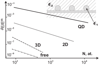
FIG. 1.: The level shift of the QD electron, calculated for 4 different depolarisation mechanisms. The giant shift, which results from the zero–point oscillations of the electric field of the QD surface mode, is shown in full line. The shifts by the 2D plasmon, the matrix bulk plasmon modes and the free field are shown as dash lines. The slopes and the prefactors of these depolarisation shifts are derived analytically and explained in the text. Inset: The scheme of the QD structure to model.

The depolarisation because of the localized surface QD modes is large enough to propose an experiment supporting our model. It is easy to see that $\overline{\delta^{2}}\sim\omega^{-3}_{L}$, whence the LS depends on the mode frequency as well. Therefore, changing the optical properties of the matrix surrounding the QD, one shifts the levels. If the bare energy level, $E^{(o)}$, lies deep in the potential well, its position is nearly independent of the well depth which changes along with the matrix parameters. The deep bare level energy depends only on the well width $\sim R$. Hence, keeping the same size of the QD and covering it with the different materials, one will derive solely the depolarisation LS, since it is distinguishable from the standard space quantization LS.

V Summary

The effect of the zero–point oscillations of the free and confined electromagnetic field on the level of the confined electron in the spherical QD is reviewed. The depolarisation due to an interaction with the zero–point oscillations of the field (produced by all other valence electrons) shifts up the bare one-electron state that seems to be a counterpart for the vertex correction (electron–hole interaction, for example) which lowers the transition frequency down. It indicates that the studied effect should be taken into account for a many–body computation of a QD spectrum.

To the best of our knowledge, the scaling dependence of the depolarisation level shift for the QDs is calculated in the first time. The size dependence of the LS is different for 4 cases considered in the paper. This scaling reflects that the different densities of states work in different mechanisms of the depolarisation due to the different 3D, 2D and 0D–dimensional modes of the electric field are involved. Our model allows a theorist to skip a tedious quantum electrodynamical calculation but obtain the analytical selfconsistent estimation for the (many–body) level shift in a nanoscale system with the strong quantization. The result has not only a theoretical importance.

Although, the depolarisation decreases with the QD size in general, the localized surface electromagnetic mode (which is specific to the QD as a void in the matrix material) results in the giant level shift and is to be possibly resolved experimentally for the QD made from some hundred atoms. Another method to detect the effect could be the measurement of a deep level position in the similar QDs buried by the substances with the distinct optical characteristics. Then the localized plasmon frequency changes along with the prefactor of the depolarisation shift, which could be observed by the optical spectroscopy of the QD system.

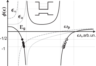
FIG. 2.: The graphical solution for the QD plasmon modes with $L\geq 1$. The solid curve gives the function to solve (see secular equation in the text). The light dotted curves represent the dielectric functions of the dot and matrix substances. The full circles are the solutions for the sphere–like modes; the open circles are the cavity–like modes (see the text). Inset: The scheme of the band structure of a QD system.

A Surface QD plasmon modes

The sought–for modes are given in complete spherical harmonics $P_{L}(r)Y_{L,M}(\Omega)$, where $P_{L}(r)$ is the Legendre polynomial and $Y_{L,M}$ is the spherical harmonic[9]. The electrodynamic solution for the modes of the system consisting of the spherical particle with the dielectric function $\epsilon_{1}(\omega)$ and the surrounding matrix with the different dielectric function $\epsilon_{2}(\omega)$ is one of the roots of the secular equation:

$$\frac{\epsilon_{2}(\omega)}{\epsilon_{1}(\omega)}=-\frac{L}{L+1}.$$ (A1)

The similar equation gives a mode of an empty void in the matrix in the limit $\epsilon_{1}=1$ (in the limit $\epsilon_{2}=1$ it gives a mode of a sphere in the vacuum). The right hand side varies from $-1/2$ to $-1$.

Let us suppose the simplest form for the dielectric function defined by one pole at some frequency, which is about the optical gap $E_{g}$, and one zero, which is given by the bulk plasma frequency of the material (both parameters differ for the materials 1 and 2). Then the solutions of the Eq.(A1) are easy to find graphically (see. Fig. 2). The function of $\omega$ standing in the left hand of the expression is plotted in solid. It has two poles at $E_{g2}$ and $\omega_{p1}$ and two zeroes at $E_{g1}$ and $\omega_{p2}$. All roots with $L=1,2..L_{c}$ lie in between these two pairs as shown in the figure. The dependence of the mode frequency on the angular momentum is very weak.

The lower–frequency modes, shown as black circles, correspond to the sphere–like plasmons. As lying above the QD gap, the lower mode effectively damps inside the QD. Therefore we will consider only the upper branch, shown as open circles, which is similar to the modes of the cavity. The frequency of the upper mode is close to the frequency of the bulk plasmon $\omega_{p2}$ as it is seen from Figure (2). The mode frequency dependence on its angular momentum is negligible.

The change of any of the 4 parameters, defining $\epsilon_{1}$ and $\epsilon_{2}$, results in the QD mode frequency shift. However, for the sought–for cavity–like mode, the most important are the plasma frequencies of the materials. This provides the mechanism for an experimental observation of the described effect in the matrix materials with the different $\omega_{p}$. It influences on the depolarisation LS, while the space quantization of the one–electron level, which is deep enough, depends solely on the QD width which has to be kept.

REFERENCES

- [1] Rotkin S.V., unpublished.
- [2] Rotkin V.V., Suris R.A., Sov.- Solid State Physics 36 (12), 1899, 1994.
- [3] Rotkin S.V., Procs of the First International Symposium on Advanced Luminescent Materials and Quantum Confinement, Eds: M. Cahay, et.al. ECS Inc., Pennington, NJ, PV 99-22, 369, 1999.
- [4] A.B. Migdal, Qualitative methods in quantum theory (Moskow: Nauka, 1975).
- [5] Ando T., Fowler A.B, Stern F., Reviews of Modern Physics, v. 54, no. 2, 4371982.
- [6] L.D. Landau, E.M. Lifshits. Electrodynamics of Continuous Media, sec.88 (Pergamon, Oxford, 1984).
- [7] A.V.Chaplik, Zh.Eksp.Teor.Fiz., 60, 1845(Sov. Phys. - JETP, 33, 997), 1971.
- [8] For the infinitely large sphere, the contraction limit is fulfilled: , but , then the (infinitely large) angular momentum can be related to the (finite) 2D wave–vector via . Substituting the maximal wave–number into this expression we get the maximal angular momentum as , where is the lattice constant. Then the critical angular momentum divided by the radius becomes some constant .
- [9] M. Abramovitz and I.A. Stegun, Handbook of Mathematical Functions (Dover, New-York, 1964).