A numerical method for detecting incommensurate correlations in the Heisenberg zigzag ladder

Abstract

We study two Heisenberg spin-1/2 chains coupled by a frustrating “zigzag” interaction. We are particularly interested in the regime of weak interchain coupling, which is difficult to analyse by either numerical or analytical methods. Previous density matrix renormalisation group (DMRG) studies of the isotropic model with open boundary conditions and sizeable interchain coupling have established the presence of incommensurate correlations and of a spectral gap. By using twisted boundary conditions with arbitrary twist angle, we are able to determine the incommensurabilities both in the isotropic case and in the presence of an exchange anisotropy by means of exact diagonalisation of relatively short finite chains of up to $24$ sites. Using twisted boundary conditions results in a very smooth dependence of the incommensurabilities on system size, which makes the extrapolation to infinite systems significantly easier than for open or periodic chains.

I Introduction

In recent years several frustrated quasi one dimensional magnetic compounds have been identified and studied experimentally [1, 2, 3, 4]. In the one-dimensional phase, i.e. for temperatures above the magnetic ordering transition, frustration is expected to lead to incommensurate correlations. Precisely how frustration gives rise to incommensurabilitites for the extreme “quantum” case of spin $S=1/2$ is at present not well understood.

A paradigm of a frustrated quantum magnet is the spin-1/2 Heisenberg antiferromagnetic chain with nearest neighbour exchange $J_{1}$ and next-nearest neighbour exchange $J_{2}$. This model is equivalent to a two-leg ladder (see Fig. 1), where the coupling along (between) the legs of the ladder is equal to $J_{2}$ ($J_{1}$).

The Hamiltonian is given by:

$$H = \sum_{i}[J_{1}(S_{i}^{x}S_{i+1}^{x}+S_{i}^{y}S_{i+1}^{y}\Delta S_{i}^{z}S_{i+1}^{z})$$ (2)

$$+\sum_{i}J_{2}(S_{i}^{x}S_{i+2}^{x}+S_{i}^{y}S_{i+2}^{y}+\Delta S_{i}^{z}S_{i+2}^{z})],$$

where we have allowed for an exchange anisotropy $\Delta$.

FIG. 1.: Schematic representation of a zig-zag ladder (top) and its equivalent chain with first and second nearest-neighbor exchange interactions (bottom).

The zigzag ladder model is believed to describe the quantum magnet ${\rm SrCuO_{2}}$ [1, 2] above the magnetic ordering transition. The ratio of exchange constants is estimated as $|J_{1}/J_{2}|\approx 0.1-0.2$ [2], so that the interchain coupling is significantly smaller than the exchange along the legs of the ladder. A second well-studied material with zigzag structure is ${\rm Cs_{2}CuCl_{4}}$ [3]. However, in ${\rm Cs_{2}CuCl_{4}}$ the chains appear to be coupled in an entire plane and no pronounced ladder structure is present.

The model (2) in the regime $J_{2}{>\atop\sim}J_{1}$ has been studied previously using both numerical [7, 8] and field-theoretical [8, 9, 10, 11, 12] methods. The main DMRG results for the spin rotationally symmetric case ($\Delta=1$) and not too large values of $J_{2}/J_{1}$ are the following [8]

• The ground state is doubly degenerate and is characterized by a nonzero dimerisation $d=\langle\vec{S}_{2n}\cdot\left(\vec{S}_{2n-1}-\vec{S}_{2n+1}\right)\rangle$.

• The equal-time correlation function $\langle\vec{S}_{n}\cdot\vec{S}_{1}\rangle$ exhibits an oscillating exponential decay at large spatial separations. The characteristic angle associated with these oscillations, i.e. the incommensurability, is related to the correlation length $\xi$ by

  $$\frac{\theta}{\pi/2}-1=\frac{1}{2\xi}.$$ (3)

  This connection of incommensurability and correlation length also fits into the picture emerging from the renormalisation group analysis (valid in the limit $J_{2}\gg J_{1}$) of [9], which yields the simultaneous divergence, with fixed ratio, of the related coupling constants.

The regime $J_{2}\gg J_{1}$ is very difficult to analyse numerically as both the dimerisation and the incommensurability become very small. In particular, the DMRG analysis of [8] did not consider this regime. At the same time the field theory studies of [9] suggest that for $J_{2}\gg J_{1}$ and $|\Delta|<1$ a different type of physics may emerge: there are still incommensurate correlations and dimerisation, but in addition there is also “chiral” order

$$\langle{S}^{+}_{2n}{S}^{-}_{2n+2}-{S}^{-}_{2n}{S}^{+}_{2n+2}\rangle\neq 0\ ,$$ (4)

$$\langle{S}^{+}_{2n}{S}^{-}_{2n-1}-{S}^{-}_{2n}{S}^{+}_{2n-1}\rangle\neq 0\ .$$ (5)

Such type of order is forbidden in the isotropic case $\Delta=1$. It clearly would be interesting to numerically analyse whether or not such a new phase indeed exists. Given the difficulties, mainly due to finite-size effects, in accessing the relevant parameter regime by numerical methods, we propose in essence to utilise finite-size effects to extract information on the incommensurability present in the system. This is done by studying the effects of twisted boundary conditions on the energy levels. Our main purpose is to establish the viability of our method by carrying out exact diagonalisation of finite clusters of up to 24 sites. In order to obtain definitive results on the zigzag chain in the most interesting parameter regime, larger systems need to be studied, possibly by implementing TBA into a DMRG algorithm.

II The method

We found the ground state of the system by Lanczos diagonalization of rings of size $L=12$, 16, 20 and 24 sites in the subspaces of total spin projection $S^{z}=0$, 1, for each total wave number $K$. We used twisted boundary conditions (TBC) $S_{i+L}^{-}=e^{i\Phi}S_{i}^{-}$. This means that each time a spin down traverses one particular link, it acquires a phase $e^{i\Phi}$ ($e^{-i\Phi})$ if it moves to the right (left). In the fermionic representation, after a Wigner-Jordan transformation $S_{i}^{-}=c_{i}^{\dagger}\exp(i\pi\sum_{j<i}c_{j}^{\dagger}c_{j})$, and a gauge transformation $c_{i}^{\dagger}=e^{i\Phi/L}f_{i}^{\dagger}$, the problem becomes equivalent to a system of $N_{\downarrow}$ fermions ($f$) on a ring threaded by a flux $\Phi$, where $N_{\downarrow}$ is the number of spins down. The advantage of the TBC for our purposes is that the allowed total wave vectors are:

$$K_{n}(\Phi)=\frac{2\pi}{L}n+\frac{\Phi}{L}N_{\downarrow},$$ (6)

with $n$ integer. Thus, varying $\Phi$, we have access to a continuum of possible wave vectors, even if we are working on a finite system [5]. As an example, the ground state of Eq. (2) for $N_{\downarrow}=1$ is known exactly. In the thermodynamic limit, for $1/4<\alpha=J_{2}/J_{1}<1/2$, the ground state is two fold degenerate with incommensurate wave vectors $K=\pm\arccos[-1/(4\alpha)]$ [6]. For small systems, these wave vectors are only accessible for discrete particular values of $\alpha$ if PBC are used. Instead, for any $\alpha$, the exact $K$’s and ground state energies are reproduced, if the energy of a small ring is minimized as a function of flux $\Phi$ and discrete wave number ($n$).

For $|\Delta|\eqslantless 1$, the transverse spin correlations dominate at large distances. We denote the ground state of the system by $|g\rangle$. It lies in the $S^{z}=0$ sector and its wave vector for PBC (or TBC if the energy is minimized over $\Phi$) is always $K_{0}=0$ or $\pi$. For the transverse spin correlations we can write:

$$C(l)=\langle g|S_{i}^{+}S_{i+l}^{-}|g\rangle=\frac{1}{L}\sum_{e,q}e^{-iql}|\langle e|S_{q}^{-}|g\rangle|^{2},$$ (7)

where $S_{q}^{-}$ is the Fourier transform of $S_{l}^{-}$, and the sum over $|e\rangle$ runs over all excited states.

By symmetry, for each $q$, only excited states with $S^{z}=-1$ and $K_{1}=K_{0}+q$ have nonvanishing matrix elements in Eq. (7). We now assume that the large-distance asymptotics of $C(l)$ is determined by the lowest excited state in the $S^{z}=-1$ sector. The difference in wave number between this state and the ground state then gives the incommensurability $q_{\min}$.

For a finite system, in order to represent a continuum of wave vectors, we minimize the energy in the $S^{z}=-1$ sector $E_{1}(K_{1},\Phi)$, as a function of flux and allowed discrete wave vectors for this flux (see Eq. (6)). The wave vector of the excitation is taken as:

$$q_{\min}=\theta=K_{1}(\Phi_{\min})-K_{0}(\Phi_{\min}),$$ (8)

where $\Phi_{\min}$ is the flux which minimizes $E_{1}(K_{1},\Phi)$, and $K_{i}(\Phi)$ is the wave vector of the state of lowest energy in the $S^{z}=-1$ sector at flux $\Phi$. The wave vector $q_{\min}$ gives the period of the oscillations of the spin correlations and corresponds to the pitch angle $\theta$ of the classical spiral density wave [7].

We have also investigated the energy gap of the spectrum. For a finite system we evaluate it as:

$$\Delta_{g}=E_{1}(K_{1},\Phi_{\min})-E_{0}(K_{0},\Phi_{\min}^{\prime}).$$ (9)

Here $\Phi_{\min}^{\prime}$ is the flux which minimizes the ground-state energy $E_{0}$. There are alternative expressions to $q_{\min}$ and $\Delta_{g}$ which converge to the same value in the thermodynamic limit. Our experience suggests that the ones we chose have the fastest convergence.

To test the method, we have studied a dimerized half filled system of non interacting spinless fermions. This model is the fermionic version of an $XY$ model plus additional interactions:

$$H_{t} = -\sum_{l=1}^{4}t_{l}\sum_{i}(c_{i+l}^{\dagger}c_{i}+{\rm H.c.})$$ (11)

$$+\frac{V}{2}\sum_{i}(-1)^{i}(c_{i+1}^{\dagger}c_{i}+{\rm H.c.}).$$

We have taken the parameters $t_{1}=1$, $t_{2}=0.4$, $t_{3}=0$, $t_{4}=-0.2$, $V=0.3$, in such a way that the upper (empty) band has minima at incommensurate wave vectors $q_{\min}=\pm 0.2356$ $\pi$, and the lower (full) band has its maximum at $q=0$. There is an indirect gap $\Delta_{g}=0.12477$.

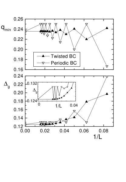
FIG. 2.: Incommensurate wave vector (top) and gap (bottom) as a function of system size, obtained using periodic and twisted boundary conditions, for the toy model Eq. (8).

In Fig. 2, we compare the results for $q_{\min}$ and $\Delta_{g}$ in finite systems of $L$ sites, with $L/4$ integer, and $12\leqslant L\leqslant 64$, between PBC and TBC. The gap is calculated as $\Delta_{g}=E_{1}(\Phi_{1})+E_{-1}(\Phi_{-1})-2E_{0}(\Phi_{0})$, where $E_{i}(\Phi_{i})$ is the ground-state energy for $i$ added particles. For TBC the fluxes $\Phi_{i}$ are those which minimize $E_{i}(\Phi_{i})$, while for PBC $\Phi_{i}=0$. Since $q_{\min}$ is near $\pi/4$, and the latter is one of the allowed wave vectors of PBC for $L$ multiple of 8, small periodic systems with $L/8$ integer have the minimum energy for one added particle, when this particle has wave vector $\pm\pi/4$. As long as $2\pi/L$ is larger than $\pi/4-|q_{\min}|$ (small systems), the results for PBC are better if $L$ is multiple of 8. However, the oscillations with increasing $L$ for PBC make a finite-size scaling difficult. Although $q_{\min}$ also oscillates with $L$ for TBC, the oscillations are smaller and the convergence to the thermodynamic limit is much faster. Using TBC, for $L\eqslantgtr 52$, the error in $q_{\min}$ and $\Delta_{g}$ are below 0.01%. For the maximum size of the system used in our Lanczos diagonalization of Eq. (2) ($L=24$), the error in $q_{\min}$ is $\sim 2\%$ and that of $\Delta_{g}$ is of the order of 10%.

III Results

1 a) Isotropic case

The incommensurate spin correlations and spin gap for $\Delta=1$ and $J_{2}/J_{1}<3$ have been studied previously by DMRG [7, 8]. In this section, we compare our results with these ones, and extend the study to $3\leq J_{2}/J_{1}\leq 30,$ a region which is very difficult to reach with other methods.

We have used a linear extrapolation in $1/L$ of the data for the angle $\theta=q_{\min}$ for $L=12,16,20,$ and $24$. We have chosen $L/4$ to be an integer in order to avoid frustration of antiferromagnetic interactions for large $J_{2}$. A quadratic fit gives smaller values of $\theta$, which underestimate the DMRG results. The comparison of available DMRG results and those obtained using TBC as described in the previous section is included in Fig. 3. For $J_{2}/J_{1}<0.7$ we do not obtain any incommensurability. This is probably a finite size effect, since for $J_{2}/J_{1}=0.7$, we obtain $\theta=\pi$ for $L=12$, but incommensurate values of $\theta$ for $L>12$. We have disregarded the value for $L=12$ in the extrapolation when $J_{2}/J_{1}=0.7$.

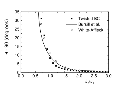
FIG. 3.: Incommensurate angle as a function of $J_{2}/J_{1}$ for $\Delta=1$, obtained using twisted boundary conditions. The DMRG results of Refs. 7,8 are also shown.

For $J_{2}/J_{1}\leq 1$ and $J_{2}/J_{1}\geq 1.8$ our results are in better agreement with those of White and Affleck [8] than with those of Bursill et al [7]. In the remaining region both DMRG results are very similar. In general, the difference between the nearest of the results of the three calculations for $\theta-90^{\circ}$ is of the order of $20\%$. For example for $J_{2}/J_{1}=0.7$ our results and those of Ref.[8, 7] are respectively 31^∘, 28^∘ and 21^∘. For $J_{2}/J_{1}=2$ the corresponding values are 1.00^∘, 1.19^∘, and 1.36^∘ . In general, comparison with DMRG results and the difference between different extrapolation methods suggest that the error in $\theta-90^{\circ}$ using TBC is roughly of the order of 20%. In view of the simplicity of our method compared to DMRG calculations, we believe that our results are satisfactory. Note that to detect an incommensurability of 1^∘ without using TBC, the size of the system should be of the order of $L\sim 360$ !

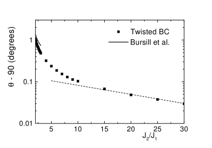
FIG. 4.: Same as Fig. 2 for $J_{2}/J_{1}>2$ in logarithmic scale. Dashed line is the function $e^{-2-0.05J_{2}/J_{1}}$.

In Fig. 4, we show the angle as a function of $J_{2}/J_{1},$ for $2\leq J_{2}/J_{1}\leq 30$ on a logarithmic scale. In this region the incommensurability is very small, and therefore, as explained above, very hard to obtain by alternative numerical methods. For large $J_{2}/J_{1}$, the deviation of the angle from $\pi/2$ is expected to be of the form [8, 9]

$$\theta-90^{\circ}=\exp(-a-bJ_{2}/J_{1})$$ (12)

A linear fit of $\ln(\theta-90^{\circ})$ as a function of $J_{2}/J_{1}$ in the interval [15,30] gives within a few percent $a=2$, and $b=1/20.$

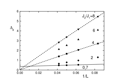
FIG. 5.: Size dependence of the gap for $\Delta=1$ and several values of $J_{2}/J_{1}$. Dashed (full) lines are quadratic (linear) fits of the data.

We have also used (9) to study the gap $\Delta_{g}$. Due to the smallness of the gap, the finite-size effects for the relatively small system sizes we consider are too large to allow us to obtain reliable values for $\Delta_{g}$. Fig. 5 shows the size dependence of $\Delta_{g}$. From the difference between linear and quadratic extrapolation, we estimate the error in the extrapolated gap to be of the order of $0.1J_{1}$, while for any value of $J_{2}/J_{1}$, $\Delta_{g}<0.5J_{1}$. Within this error, our results agree with those reported by White and Affleck [8].

2 b) Anisotropic case

In [9] the zigzag ladder was studied by means of a field theory approach in the regime $J_{2}\gg J_{1}$. A mechanism for generating incommensurabilities was identified and analysed quantitatively for the case of two coupled XX chains ($\Delta=0$). It was found that spin correlations exhibit a very slow power-law decay and are incommensurate

$$\langle S_{1}^{+}(x)S_{j}^{-}(0)\rangle\sim\frac{(-1)^{x/a_{0}}}{|x|^{1/4}}\ \exp\left[-i\kappa x/a_{0}\right]$$ (13)

where $j=1,2$ and the deviation of the pitch angle from $\pi$ is $\kappa\propto(J_{1}/J_{2})^{2}$. The analysis of [9] also implies the existence of local magnetisation currents around the elementary triangular plaquettes of the ladder. The findings of [9] were questioned in [13], where the squares of the local magnetisation currents were computed numerically and found to decrease with system size for open chains of up to 16 sites.

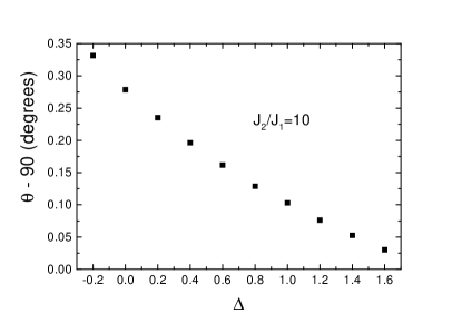
FIG. 6.: Incommensurate angle as a function of $\Delta$ for $J_{2}/J_{1}=10.$

In an attempt to resolve this controversy we have set $J_{2}/J_{1}=10$ and studied the variation of the incommensurate angle with the anisotropy parameter $\Delta$. As shown in Fig. 6, we find that $\theta-90^{\circ}$ increases considerably as $\Delta$ is decreased from the isotropic case $\Delta=1$. This is in agreement with the field-theory prediction of [9].

We futhermore have determined the dependence of the incommensurability on $J_{2}/J_{1}$. The results are shown in Fig. 7. For large values of $J_{2}/J_{1}$ our numerical results are well fitted by

$$\theta-90^{\circ}=2.785^{\circ}\frac{J_{1}}{J_{2}}\ .$$ (14)

This is in disagreement with the prediction of [9].

The disagreement between the predictions of [9] and the numerical results (14) and [13] could either be due to a defect in the mean-field solution of [9] or be an artifact of the limited system sizes used in the numerical computations. In fact, the analysis of [9] predicts a gapless phase at $\Delta=0$ so that it is conceivable that numerical results for small clusters are plagued by finite-size effects.

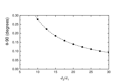
FIG. 7.: Incommensurate angle as a function of $J_{2}/J_{1}$ for $\Delta=0$. Dashed line is the function $2.785^{\circ}J_{1}/J_{2}$.

There is indeed evidence suggesting that finite-size effects are still significant for $L=24$. We find that the ground state in the $S^{z}=1$ sector has a lower energy than the first excited state in the $S^{z}=0$ sector for $L=24$ and ${J_{2}}{\stackrel{{\scriptstyle\textstyle>}}{{\sim}}}2J_{1}$. On the other hand, the DMRG studies of [8] show that in the isotropic case and for long lattices the two lowest levels are both in the $S^{z}=0$ sector (degenerate ground states corresponding to different signs of the dimerisation).

We note that the presence of such finite-size effects does not necessary imply that the extrapolated results for the incommensurability are incorrect. In order to resolve this issue it is necessary to study significantly longer lattices.

IV Summary and discussion

We have calculated the incommensurate wave number in the next-nearest-neighbor Heisenberg model with anisotropy $\Delta$, by exact diagonalization of rings of up to 24 sites. We have used twisted boundary conditions and assumed that the incommensurate spin fluctuations for $|\Delta|\eqslantless 1$ are determined by the lowest excited state for total spin projection $S^{z}=\pm 1$.

The method is able to detect incommensurate angles $\theta\sim 0.03^{\circ}$. This corresponds to a wave length of the order of 10 000 sites and is impossible to detect by using alternative numerical methods. However, for certain parameters ($J_{2}/J_{1}<0.7$ in the model), our method is unable to detect the incommensurability although it is rather large. On the other hand, the method does not predict incommensurabilities in cases where it is known that none exist. Also, in general, the extrapolated vales of $\theta$ seem to be underestimations, as compared with known DMRG results. This is also the case for the toy model (Eq. (11)), represented in Fig. 2, where a linear extrapolation gives an underestimation of $q_{\min}$ by $\sim 30\%$ if the results are limited to 24 sites.

The advantage of using TBC for facilitating a finite-size scaling analysis has been noted previously in e.g. [14], but their use for detecting incommensurabilities is to the best of our knowledge novel.

In spite of the limitations of the size of the cluster, the values of $\theta$ obtained with our method are in reasonable agreement with known DMRG results in the isotropic case. For this case, we have also studied the region $J_{2}/J_{1}>3$, which is very difficult to reach by alternative methods. For sufficiently large $J_{2}/J_{1}$, $\theta-\pi/2$ decays as $\exp(-b$ $J_{2}/J_{1})$ as predicted by field theory [8]. We obtain that the constant $b\sim 1/20$.

In the anisotropic case, we obtain that $\theta$ increases with decreasing $\Delta$, in agreement with Ref. [9]. However, we find a linear dependence of $\theta-\pi/2$ on $J_{1}/J_{2}$ for $J_{2}\gg J_{1}$, in contrast to the quadratic behaviour predicted in [9]. This discrepancy may be due to finite-size effects.

In summary, we have shown that incommensurabilities can be detected by diagonalizing finite-size clusters with TBC. The main advantage of the method is that the dependence of the incommensurability on system size is very smooth and allows extrapolation from results for relatively short chains.

It would be very interesting to implement our TBC method in a DMRG algorithm and study the anisotropic zigzag chain for much larger sizes.

REFERENCES

-
[1]
M. Matsuda and K. Katsumata, J. Mag. Mag. Mat. 140, 1617 (1995),
Z. Hiroi, M. Azuma, M. Takano and Y. Bando, J. Solid State Chem. 95, 230 (1991);
N. Motoyama, H. Eisaki and S. Uchida, Phys. Rev. Lett. 76, 3212 (1996). - [2] M. Matsuda, K. Katsumata, K.M. Kojima, M. Larkin, G.M. Luke, J. Merrin, B. Nachumi, Y.J. Uemura, H. Eisaki, N. Motoyama, S. Uchida and G. Shirane, Phys. Rev. B55, R11953 (1997).
-
[3]
R. Coldea
R. Coldea, D.A. Tennant, R.A. Cowley, D.F. McMorrow, B. Dorner and
Z. Tylczynski, Phys. Rev. Lett. 79, 151 (1997),
R. Coldea and D.A. Tennant, private communications. - [4] D.C. Johnston et al, unpublished, preprint cond-mat/0001147.
- [5] L. Arrachea, A. A. Aligia and E. R. Gagliano, Phys. Rev. Lett. 76, 4396 (1996).
- [6] For example C. Gerhardt, K.-H. Mütter and H. Kröger, Phys. Rev. B 57, 11 504 (1998).
- [7] R. Bursill, G.A. Gehring, D.J.J. Farnell, J.B. Parkinson, T. Xiang and C. Zeng, J. Phys. Cond. Mat 7, 8605 (1995).
- [8] S. R. White and I. Affleck, Phys. Rev. B 54, 9862 (1996).
- [9] A. A. Nersesyan, A. O. Gogolin, and F. H. L. Eßler, Phys. Rev. Lett 81, 910 (1998).
- [10] D. Allen and D. Sénéchal, Phys. Rev. B55, 299 (1997).
- [11] D. Allen, F.H.L. Essler and A.A. Nersesyan, to appear in Phys. Rev. B.
- [12] D. Cabra, A. Honecker and P. Pujol, Eur. Phys. Jour. B13, 55 (2000).
- [13] M. Kaburagi, H. Kawamura, and T. Hikihara, J. Phys. Soc. Jpn 68, 3185 (1999).
- [14] G. Fath and J. Solyom, Phys. Rev. B47, 872 (1992).