Steady-state mode I cracks in a viscoelastic triangular lattice

Abstract

We continue our study of the exact solutions for steady-state cracks in ideally brittle viscoelastic lattice models by focusing on mode I in a triangular system. The issues we address include the crack velocity versus driving curve as well as the onset of additional bond-breaking, signaling the emergence of complex spatio-temporal behavior. Somewhat surprisingly, the critical velocity for this transition becomes a decreasing function of the dissipation for sufficiently large values thereof. At the end, we briefly discuss the possible relevance of our findings for experiments on mode I crack instabilities.

Keywords: Crack Propagation and Arrest, Dynamic Fracture, Crack Branching and Bifurcation

I Introduction

In the previous paper (Pechenik, et al., 2000), we showed how one could extend the methodology originally devised by Slepyan (1981) and obtain a closed form solution for mode III cracks propagating steadily in a square lattice in the presence of dissipation in the form of a Kelvin viscosity. This approach allowed us to determine the effect of dissipation on the crack velocity as a function of driving. Similarly, we found the critical velocity (and the associated critical time) at which other bonds in the lattice have displacements larger than the assumed breaking criterion, signaling an instability in the steadily-propagating crack and the onset of more complex spatio-temporal behavior.

In this second paper, we extend this analysis to the more interesting (and more experimentally relevant) case of mode I cracks. We now work on a triangular lattice and assume that there are central force ideally brittle viscoelastic springs connecting particles at the lattice sites. Again, we use ideas borrowed from Kulamekhtova (1984) to solve this problem exactly on an infinite lattice. We also solve the same system numerically on a lattice of finite transverse extent so as to provide an independent check on some of the results.

Perhaps the most interesting finding reported here concerns the aforementioned onset of additional bond-breaking at large enough velocity. At small dissipation, diagonal bonds that are offset from the assumed crack line in the vertical direction are the most “dangerous”. The critical velocity at which one of these bonds exceeds critical displacement is more or less independent of the dissipation at low values thereof and eventually rises sharply as the system becomes increasingly damped. This is similar to the behavior obtained for mode III. At moderate to large damping, however, horizontal bonds become more relevant and eventually give rise to a critical velocity which decreases with increasing damping. At the end, we will comment on the possible relevance of our results for trying to make sense of recent experiments (Fineberg, et al., 1991, 1992; Sharon, et al., 1995, 1996) and simulations on instabilities during dynamic fracture.

II Mode I on a triangular lattice

Our model consists of central force springs between mass points located on a triangular lattice. We introduce unit vectors in the lattice directions as follows: $\hat{d}_{1}$ points in the direction of the $x$-axis and each of the subsequent unit vectors $\hat{d}_{i}$ with $2\leq i\leq 6$ rotated by an additional $\pi/3$ in the counter-clockwise direction. This means that $\hat{d}_{i+3}=-\hat{d}_{i}$. We will always assume that the steady-state crack breaks bonds between the rows with $y=0$ and $y=\sqrt{3}/2$, as it moves in the direction of the $x$-axis.

As already discussed in our previous paper on mode III cracks, each bond is taken to be linear until a critical displacement at which point it completely breaks. Also, dissipation is incorporated as a Kelvin viscosity term. Given these assumptions, the equation describing the motion of the masses in the lattice is

$$(1+\eta\frac{\partial}{\partial t})\sum_{i=1}^{6}Q_{i}(t,\vec{x})\hat{d}_{i}-\frac{\partial^{2}\vec{u}(t,\vec{x})}{\partial t^{2}}=-\vec{\sigma}(t,\vec{x})\ .$$ (1)

Here, $\vec{x}=(x,y)$ is a lattice vector in the plane and $Q_{i}(t,\vec{x})$ is the elongation of bond $i$ emanating from the specific lattice site, in the approximation that this elongation is much smaller than the unstretched bond length,

$$Q_{i}(t,\vec{x})=\left(\vec{u}(t,\vec{x}+\hat{d}_{i})-\vec{u}(t,\vec{x})\right)\cdot\hat{d}_{i}\ .$$ (2)

Finally, the driving term $\vec{\sigma}(t,\vec{x})$ consists of forces which compensate for the forces from broken bonds (which are included on the left-hand side) as well as any external forces acting on the crack boundaries.

Next we suppose that the crack is moving with a constant speed $v$. This allows us to change variables to $\tau=x-vt$, $\vec{z}=(\tau,y)$, which gives

$$(1-\eta v\frac{\partial}{\partial\tau})\sum_{i=1}^{6}Q_{i}(\vec{z})\hat{d}_{i}-v^{2}\frac{\partial^{2}\vec{u}(\vec{z})}{\partial\tau^{2}}=-\vec{\sigma}(\vec{z})\ .$$ (3)

Because of the form of $Q_{i}(\vec{z})$, we have the obvious symmetries

$$Q_{2}(\vec{z})=Q_{5}(\vec{z}+\hat{d}_{2}),\;Q_{3}(\vec{z})=Q_{6}(\vec{z}+\hat{d}_{3})\ .$$ (4)

We will impose one additional symmetry condition on the $Q_{i}$. As the crack propagates, it alternately breaks bonds in the $\hat{d}_{2}$ and $\hat{d}_{3}$ directions. Let us define our coordinates such that at $\tau=0$ and $t=0$, (so that $x=0$), the crack breaks a bond in the direction of $\hat{d}_{2}$. This means that for $\tau>0$ this bond ($Q_{2}(\vec{z}_{0})$ with $\vec{z}_{0}=(\tau,0)$) is unbroken and for $\tau<0$ it is always broken. If we shift one lattice spacing to the left, the $\hat{d}_{2}$ bond at $x=-1$ will break at $t=-1/v$ (here also $\tau=0$ in $Q_{2}(\vec{z}_{0})$). It is clear that the bond in the $\hat{d}_{3}$ direction at $x=0$ breaks at a time-point between these two events; we will assume that this time is exactly at the midpoint, $t=-1/(2v)$ or equivalently $\tau=1/2$ in $Q_{3}(\vec{z}_{0})$. This means that for $\tau>1/2$ this bond is unbroken and for $\tau<1/2$ it is always broken. We will assume an even more strict symmetry condition for these bonds, namely

$$Q_{2}(\vec{z}_{0})=Q_{3}(x-v(t-\frac{1}{2v}),y=0)=Q_{3}(\vec{z}_{0}+\frac{1}{2}\hat{d}_{1})$$ (5)

which will need to be checked from our solution later.

Let us denote $Q_{2}(\vec{z}_{0})\equiv Q(\tau)$. Then, we can write down an explicit expression for the forces $\vec{\sigma}(z)$ on the right hand side of Eq. 3. For the row with $y=0$

$$\vec{\sigma}(\vec{z}_{0}) = \theta(-\tau)\left(\vec{\sigma}_{e}(\vec{z}_{0})-(1-\eta v\frac{\partial}{\partial\tau})Q_{2}(\vec{z}_{0})\hat{d}_{2}\right)$$

$$+\theta(-\tau+\frac{1}{2})\left(\vec{\sigma}_{e}\,^{\prime}(\vec{z}_{0})-(1-\eta v\frac{\partial}{\partial\tau})Q_{3}(\vec{z}_{0})\hat{d}_{3}\right)$$

$$= \theta(-\tau)\left(-P_{0}(\tau)-(1-\eta v\frac{\partial}{\partial\tau})Q(\tau)\right)\hat{d}_{2}$$

$$+\theta(-\tau+\frac{1}{2})\left(-P_{0}(\tau-\frac{1}{2})-(1-\eta v\frac{\partial}{\partial\tau})Q(\tau-\frac{1}{2})\right)\hat{d}_{3}\ .$$ (7)

Here $\vec{\sigma}_{e}$ and $\vec{\sigma}_{e}\,^{\prime}$ are the assumed external forces. In the second form, these have been taken to match the vectorial nature and also the symmetry of the bond-breaking terms. The (scalar) $P_{0}$ will be specified later. Note that the second theta-function in (II) reflects the already mentioned fact that the bond from point $\vec{z}_{0}$ in the $\hat{d}_{3}$ direction breaks earlier (by time interval $1/2v$) than the bond from the same point in the $\hat{d}_{2}$ direction.

Let us write down the corresponding force for the row $y=\sqrt{3}/2$. For the point $\vec{x}=\hat{d}_{2}$, the bond in the $\hat{d}_{5}$ direction is physically the same as the $\hat{d}_{2}$ bond at $\vec{x}=(0,0)$ and therefore breaks at $\tau=0$ in $Q_{5}(\vec{z}_{0}+\hat{d}_{2})=Q_{2}(\vec{z}_{0})$. Now, the $\hat{d}_{6}$ bond at $\vec{x}=\hat{d_{2}}$ breaks later, at $\tau=-1/2$ in $Q_{6}(\vec{z}_{0}+\hat{d}_{2})$. Thus we have

$$\vec{\sigma}(\vec{z}_{0}+\hat{d}_{2}) = \theta(-\tau)\left(\vec{\sigma}_{e}(\vec{z}_{0}+\hat{d}_{2})-(1-\eta v\frac{\partial}{\partial\tau})Q_{5}(\vec{z}_{0}+\hat{d}_{2})\hat{d}_{5}\right)$$

$$+\theta(-\tau-\frac{1}{2})\left(\vec{\sigma}_{e}^{\prime}(\vec{z}_{0}+\hat{d}_{2})-(1-\eta v\frac{\partial}{\partial\tau})Q_{6}(\vec{z}_{0}+\hat{d}_{2})\hat{d}_{6}\right)$$

$$= \theta(-\tau)\left(-P_{0}(\tau)-(1-\eta v\frac{\partial}{\partial\tau})Q(\tau)\right)\hat{d}_{5}+$$

$$+\theta(-\tau-\frac{1}{2})\left(-P_{0}(\tau+\frac{1}{2})-(1-\eta v\frac{\partial}{\partial\tau})Q(\tau+\frac{1}{2})\right)\hat{d}_{6}\ .$$ (9)

where we used the symmetry in Eq. 5 to write $Q_{6}(\vec{z}_{0}+\hat{d}_{2})=Q_{3}(\vec{z}_{0}+\hat{d}_{2}-\hat{d}_{3})=Q_{2}(\vec{z}_{0}+\hat{d}_{2}-\hat{d}_{3}-\hat{d}_{1}/2)=Q(\tau+1/2)$. Finally, we can rewrite all these forces in a more compact form,

$$\vec{\sigma}(\vec{z}_{0}) = N(\tau)\hat{d}_{5}+N(\tau-\frac{1}{2})\hat{d}_{6}\ ,$$ (10)

$$\vec{\sigma}(\vec{z}_{0}+\hat{d}_{2}) = N(\tau)\hat{d}_{2}+N(\tau+\frac{1}{2})\hat{d}_{3}\ ,$$ (11)

where

$$N(\tau)=\theta(-\tau)\left(P_{0}(\tau)+(1-\eta v\frac{\partial}{\partial\tau})Q(\tau)\right)\ .$$ (12)

Next, we proceed by doing a Fourier transformation of Eq. (3), over the continuous variable $\tau$ and the discrete variable $y=n\sqrt{3}/2$, with integer $n$. In detail,

$$u^{F}(\tau,s) = \sum_{n=-\infty}^{+\infty}u\left(\tau,\frac{\sqrt{3}}{2}n\right)e^{i\frac{\sqrt{3}}{2}sn}\ ,$$ (13a)

$$u(\tau,y) = \frac{\sqrt{3}}{4\pi}\int_{-\frac{2\pi}{\sqrt{3}}}^{\frac{2\pi}{\sqrt{3}}}u^{F}(\tau,s)e^{-isy}ds\ ;$$ (13b)

$$u^{FF}(q,s) = \int_{-\infty}^{+\infty}u^{F}(\tau,s)e^{iq\tau}d\tau\ ,$$ (14a)

$$u^{F}(\tau,s) = \frac{1}{2\pi}\int_{-\infty}^{+\infty}u^{FF}(q,s)e^{-iq\tau}dq\ .$$ (14b)

We thereby obtain

$$-v^{2}q^{2}\vec{u}^{FF}-(1+i\eta vq)\sum_{i}Q_{i}^{FF}\hat{d}_{i}=\vec{\sigma}^{FF}\ ,$$ (15)

with

$$Q_{i}^{FF}=(e^{-i\vec{r}\cdot\hat{d}_{i}}-1)\vec{u}^{FF}\cdot\hat{d}_{i}$$ (16)

and $\vec{r}=(q,s)$.

To find $\vec{\sigma}^{FF}$ we first transform Eqs. (10, 11) over $\tau$

$$\vec{\sigma}^{F}(q,n=0) = N(q)\hat{d}_{5}+e^{i\frac{q}{2}}N(q)\hat{d}_{6}\ ,$$ (17a)

$$\vec{\sigma}^{F}(q,n=1)e^{-i\frac{q}{2}} = N(q)\hat{d}_{2}+e^{-i\frac{q}{2}}N(q)\hat{d}_{3}\ ,$$ (17b)

with

$$N(q)=P_{0}^{-}+(1+i\eta vq)Q^{-}-\eta vQ(0)\ .$$ (18)

The superscript “$-$” refers to the part of the Fourier transform which is analytic in the lower half plane of the variable $q$; our notation follows that in our previous mode III paper. Finally, using (13a) we get

$$\vec{\sigma}^{FF}=N(q)\hat{d}_{5}+e^{i\frac{q}{2}}N(q)\hat{d}_{6}+\left(e^{i\frac{q}{2}}N(q)\hat{d}_{2}+N(q)\hat{d}_{3}\right)e^{is\frac{\sqrt{3}}{2}}\ .$$ (19)

This then completes the derivation of the basic equation that needs to be solved to determine the steady-state crack field.

III Wiener-Hopf Solution

We wish to use the Wiener-Hopf technique to solve the equation derived above for the elongation field $Q$. To start, we note that Eq. (15) can be written in matrix form

$${\bf M}\vec{u}^{FF}=\vec{\sigma}^{FF}$$ (20)

with the 2x2 matrix

$$\bf{M}=\left(\begin{array}[]{clrr}A_{1}&A_{3}\\ A_{3}&A_{2}\end{array}\right)$$ (21)

where

$$A_{1} = -v^{2}q^{2}+(1+i\eta vq)\left(4\sin^{2}\frac{\vec{r}\cdot\hat{d}_{1}}{2}+\sin^{2}\frac{\vec{r}\cdot\hat{d}_{2}}{2}+\sin^{2}\frac{\vec{r}\cdot\hat{d}_{3}}{2}\right)\ ,$$ (22a)

$$A_{2} = -v^{2}q^{2}+3(1+i\eta vq)\left(\sin^{2}\frac{\vec{r}\cdot\hat{d}_{2}}{2}+\sin^{2}\frac{\vec{r}\cdot\hat{d}_{3}}{2}\right)\ ,$$ (22b)

$$A_{3} = \sqrt{3}(1+i\eta vq)\left(\sin^{2}\frac{\vec{r}\cdot\hat{d}_{2}}{2}-\sin^{2}\frac{\vec{r}\cdot\hat{d}_{3}}{2}\right)\ ,$$ (22c)

and

$$\vec{\sigma}^{FF}=-\frac{N(q)}{2}\left(\begin{array}[]{clrr}(1-e^{i\frac{q}{2}})(1+e^{i\frac{\sqrt{3}}{2}s})\\ \sqrt{3}(1+e^{i\frac{q}{2}})(1-e^{i\frac{\sqrt{3}}{2}s})\end{array}\right)\ .$$ (23)

The solution of (20) is therefore

$$\vec{u}^{FF}=\frac{1}{\det{\bf M}}\left(\begin{array}[]{clrr}\det{\bf M}_{1}\\ \det{\bf M}_{2}\end{array}\right)$$ (24)

where

$${\bf M}_{1}=\left(\begin{array}[]{clrr}\sigma^{FF}_{x}&\sigma^{FF}_{y}\\ A_{3}&A_{2}\end{array}\right)\ ,\;\;\;\;{\bf M}_{2}=\left(\begin{array}[]{clrr}A_{1}&A_{3}\\ \sigma^{FF}_{x}&\sigma^{FF}_{y}\end{array}\right)\ .$$ (25)

Now, we want to extract from the solution (24) an equation for the variable we are interested in, namely $Q^{F}(q)$. From the definition of $Q$ we have

$$Q^{F}(q)=Q_{2}^{F}(q,n=0)=\frac{\sqrt{3}}{4\pi}\int_{-\frac{2\pi}{\sqrt{3}}}^{\frac{2\pi}{\sqrt{3}}}(e^{-i\vec{r}\cdot\hat{d}_{2}}-1)\vec{u}^{FF}\cdot\hat{d}_{2}\ ds\ .$$ (26)

From the basic solution above, we can evaluate $\vec{u}^{FF}\cdot\hat{d}_{2}$.

$$\vec{u}^{FF}\cdot\hat{d}_{2}=\frac{\left|\begin{array}[]{clrr}-d_{2x}A_{3}+d_{2y}A_{1}&-d_{2x}A_{2}+d_{2y}A_{3}\\ \sigma^{FF}_{x}&\sigma^{FF}_{y}\end{array}\right|}{|{\bf M}|}\ .$$ (27)

Before proceeding to evaluate the integral, it is worthwhile to pause and check the basic symmetry conditions. We find that

$$Q_{3}^{F}(q,n=0)=\frac{\sqrt{3}}{4\pi}\int_{-\frac{2\pi}{\sqrt{3}}}^{\frac{2\pi}{\sqrt{3}}}(e^{-i\vec{r}\cdot\hat{d}_{3}}-1)\vec{u}^{FF}\cdot\hat{d}_{3}\ ds\ ,$$ (28)

where the new dot product is given by

$$\vec{u}^{FF}\cdot\hat{d}_{3}=\frac{\left|\begin{array}[]{clrr}d_{2x}A_{3}+d_{2y}A_{1}&d_{2x}A_{2}+d_{2y}A_{3}\\ \sigma^{FF}_{x}&\sigma^{FF}_{y}\end{array}\right|}{|{\bf M}|}\ .$$ (29)

Now, we can change variables of integration in (28) from $s$ to $-s$. Under this transformation $A_{1}|_{s\rightarrow-s}=A_{1}$, $A_{2}|_{s\rightarrow-s}=A_{2}$, $A_{3}|_{s\rightarrow-s}=-A_{3}$, $\sigma_{x}^{FF}|_{s\rightarrow-s}=e^{-i\sqrt{3}s/2}\sigma_{x}^{FF}$, $\sigma_{y}^{FF}|_{s\rightarrow-s}=-e^{-i\sqrt{3}s/2}\sigma_{y}^{FF}$, which gives that $\det{\bf M}|_{s\rightarrow-s}=\det{\bf M}$ and $\vec{u}^{FF}\cdot\hat{d}_{3}|_{s\rightarrow-s}=-e^{-i\sqrt{3}s/2}\vec{u}^{FF}\cdot\hat{d}_{2}$. Therefore (28) changes into

$$Q_{3}^{F}(q,n=0)=-\frac{\sqrt{3}}{4\pi}\int_{-\frac{2\pi}{\sqrt{3}}}^{\frac{2\pi}{\sqrt{3}}}(e^{iqd_{2x}+isd_{2y}}-1)e^{-id_{2y}s}\vec{u}^{FF}\hat{d}_{2}ds=e^{i\frac{q}{2}}Q_{2}^{F}(q,n=0)\ .$$ (30)

This is exactly the symmetry condition (5); hence, our solution is consistent with the assumed symmetry. We also note here that a similar derivation gives

$$Q_{2}(\tau,y)=Q_{3}(\tau+\frac{1}{2},-y)=Q_{6}(\tau+\frac{1}{2},-y+\frac{\sqrt{3}}{2})\ .$$ (31)

More generally, we can see what these symmetries mean for the displacement field $\vec{u}(z)$. Using $\det{\bf M}_{1}|_{s\rightarrow-s}=e^{-i\sqrt{3}s/2}\det{\bf M}_{1}$, $\det{\bf M}_{2}|_{s\rightarrow-s}=-e^{-i\sqrt{3}s/2}\det{\bf M}_{2}$, we obtain $u_{x}^{FF}|_{s\rightarrow-s}=e^{-i\sqrt{3}s/2}u_{x}^{FF}$ and $u_{y}^{FF}|_{s\rightarrow-s}=-e^{-i\sqrt{3}s/2}u_{y}^{FF}$. These give $u_{x}(\tau,y)=u_{x}(\tau,-y+\sqrt{3}/2)$ and $u_{y}(\tau,y)=-u_{y}(\tau,-y+\sqrt{3}/2)$.

We now proceed to calculate the integral in (26). The explicit form of the integrand in (26) is

$$\frac{N(q)}{|{\bf M}|}\,\left|\begin{array}[]{clrr}3\left(\frac{v^{2}q^{2}}{2}-(1+i\eta vq)(2\sin^{2}\frac{q}{2}+\sin^{2}\frac{\vec{r}\cdot\hat{d}_{3}}{2})\right)&-\frac{v^{2}q^{2}}{2}+3(1+i\eta vq)\sin^{2}\frac{\vec{r}\cdot\hat{d}_{3}}{2}\\ (\cos\vec{r}\cdot\hat{d}_{2}-1)-(\cos\frac{\sqrt{3}}{2}s-\cos\frac{q}{2})&(\cos\vec{r}\cdot\hat{d}_{2}-1)+(\cos\frac{\sqrt{3}}{2}s-\cos\frac{q}{2})\end{array}\right|\ .$$ (32)

As $|{\bf M}|$ is an even function of $s$, only the even part of the other determinant contributes to the integral. Then, by the change of variable to $w=e^{-i\sqrt{3}s/2}$ we can rewrite (26) as an integral over the unit circle in the complex $w$ plane. After some tedious algebra, we find that we can write

$$\det{\bf M}=3\xi^{2}+\alpha\xi+\beta$$ (33)

where

$$\xi = (1+i\eta vq)\frac{1}{2}\left(\frac{1}{w}+w\right)\ ,$$ (34a)

$$\alpha = -2\cos\frac{q}{2}\left(-2v^{2}q^{2}+3(1+i\eta vq)(1+2\sin^{2}\frac{q}{2})\right)\ ,$$ (34b)

$$\beta = 3(1+i\eta vq)^{2}(1+3\sin^{2}\frac{q}{2})-4(1+i\eta vq)v^{2}q^{2}(1+\sin^{2}\frac{q}{2})+v^{4}q^{4}\ .$$ (34c)

Similarly, the even part of the determinant in the numerator becomes

$$\frac{F(\xi)}{1+i\eta vq}\ ,$$ (35)

with

$$F(\xi) = 3\left[(\xi-(1+iq\eta v)\cos\frac{q}{2})^{2}+2(1+iq\eta v)\sin^{2}\frac{q}{2}(1+\cos\frac{q}{2})(1+iq\eta v-\xi)\right]$$ (36)

$$-v^{2}q^{2}\left[(1+iq\eta v-\xi)(1+\cos\frac{q}{2})-\xi\cos\frac{q}{2}+1+i\eta vq\right]\ .$$

We write down here also the odd part of this determinant for future reference,

$$G(w)=i(\frac{1}{w}-w)\sin\frac{q}{2}(v^{2}q^{2}-3(1+iq\eta v)\sin^{2}\frac{q}{2})\ .$$ (37)

Inserting (33) and (35) into (32) we can see that (26) becomes

$$Q^{F}(q)=\frac{N(q)}{2\pi i(1+i\eta vq)}\oint\limits_{|w|=1}\frac{F(\xi)}{3\xi^{2}+\alpha\xi+\beta}\frac{dw}{w}$$ (38)

with integration around the unit circle in the counter-clockwise direction. The integrand in Eq. (38) has three poles inside the unit circle; i.e., $w=0$ and one $w$ for each of the two roots of the expression (33),

$$\xi_{1,2}=C\pm\sqrt{C^{2}-D}\ ,$$ (39)

with

$$C = \cos\frac{q}{2}\left(-\frac{2}{3}v^{2}q^{2}+(1+i\eta vq)(1+2\sin^{2}\frac{q}{2})\right)\ ,$$ (40a)

$$D = (1+i\eta vq)^{2}(1+3\sin^{2}\frac{q}{2})-\frac{4}{3}(1+i\eta vq)v^{2}q^{2}(1+\sin^{2}\frac{q}{2})+\frac{1}{3}v^{4}q^{4}\ .$$ (40b)

Then calculating the residues at these poles we get

$$Q^{F}(q)=\frac{N(q)}{1+i\eta vq}(1-S)$$ (41)

where

$$S(q)=\frac{F(\xi_{1})\sqrt{\xi_{2}^{2}-(1+i\eta vq)^{2}}-F(y_{2})\sqrt{\xi_{1}^{2}-(1+i\eta vq)^{2}}}{3(\xi_{1}-\xi_{2})\sqrt{\xi_{1}^{2}-(1+i\eta vq)^{2}}\sqrt{\xi_{2}^{2}-(1+i\eta vq)^{2}}}\ .$$ (42)

Note that we are supposed to take those branches of the square roots in (42) which ensure that

$$|w_{1,2}|<1$$ (43)

with $w_{1,2}$ defined by

$$w_{1,2}=\frac{\xi_{1,2}-\sqrt{\xi_{1,2}^{2}-(1+i\eta vq)^{2}}}{1+i\eta vq}$$ (44)

If we now substitute $N(q)$ in Eq. (41) into Eq. (18), we get exactly the same equation as was obtained for the mode III case in the first paper (Pechenik, et al., 2000)

$$Q^{+}+SQ^{-}+\frac{\eta v}{1+i\eta vq}(1-S)Q(0)=\frac{(1-S)P_{0}^{-}}{1+i\eta vq}$$ (45)

with $Q$ having the same meaning as $\vee$ in (Pechenik, et al., 2000), namely the elongation of bonds between rows where the crack propagates.

Therefore, we do not need to repeat any of the discussion from our previous paper regarding the choice of $P_{0}^{-}$ and the factorization into pieces analytic in the upper and lower half planes. Instead, we can just write down the final answer. For the relationship between the velocity and the driving displacement, we have

$$\frac{\Delta}{\Delta_{G}}=\sqrt{\frac{1+\phi\eta v}{A\phi}}\exp{\frac{1}{4\pi i}\int_{-\infty}^{+\infty}\frac{\ln K(\chi)}{\chi(1+i\eta v\chi)}d\chi}$$ (46)

where for this mode I case

$$A=\frac{1}{\sqrt{2}v^{2}}\left(\frac{\sqrt{\frac{3}{8}-v^{2}}}{2}-\frac{(-\frac{3}{4}+v^{2})^{2}}{\sqrt{3}\sqrt{\frac{9}{8}-v^{2}}}\right)$$ (47)

and

$$K(q)=\frac{S^{2}(q)(q^{2}+\phi^{2})}{A^{2}q^{2}\phi^{2}}\ .$$ (48)

This expression for $A$ contains the transverse speed $c_{t}=\sqrt{3/8}$ and longitudinal speed $c_{l}=\sqrt{9/8}$. The zero of $A$ gives the limiting speed of crack propagation $c_{R}=\frac{\sqrt{3-\sqrt{3}}}{2}=0.563$, which is as expected equal to the Raleigh wave speed.

In our previous paper, we discussed the details of how to evaluate this equation so as to obtain numerical results for the crack velocity response curve. These methods can be applied to this case as well and hence we do not repeat any of the details here. The results of these calculations are presented in Figs. 1 and 2. In fact, these findings are quite similar to the analogous mode III results. Later, we will show that the upper limiting value of $\Delta/\Delta_{G}$ for an arrested (i.e. non-moving) crack is around $1.94$. As was the case for mode III, the $\Delta-v$ curves in Figures 1, 2 approach this value as $v$ goes to 0 at any value of the damping $\eta$. Slepyan’s original calculations, done for the dissipationless limit $\eta=0$, show the same asymptotic value.

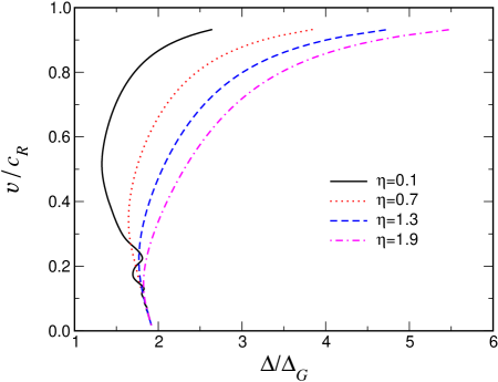
Figure 1: Dependence of $\Delta/\Delta_{G}$ on speed $v$ for $\eta=0.1$, $0.7$, $1.3$, $1.9$

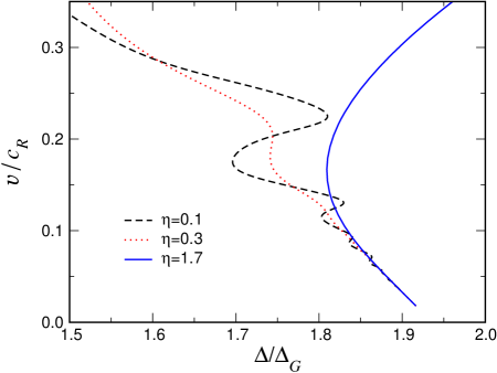
Figure 2: Change of behavior for small $\eta$. Note the rapid oscillations at smaller speeds.

IV consistency of the steady-state solution

In this section we calculate the bond displacements in the vicinity of the crack. This is crucial, as we need to check whether all bonds assumed to be unbroken in the derivation in fact have elongations less than unity, the value at which bonds break.

Let us start with bonds along the crack path, where the elongation is just determined by transforming $Q^{F}(q)$ back to physical space. This part follows exactly the analogous mode III calculation, and we easily obtain for $Q^{\pm}$

$$Q^{+} = \frac{Q(0)}{(-iq+0)(1+iq\eta v)}\frac{S^{+}}{\left.S^{+}\right|_{q=\frac{i}{\eta v}}}-\frac{\eta vQ(0)}{1+iq\eta v}\ ,$$ (49a)

$$Q^{-} = \frac{Q(0)}{\left.S^{+}\right|_{q=\frac{i}{\eta v}}S^{-}}\frac{1}{(iq+0)(1+iq\eta v)}+\frac{\eta vQ(0)}{1+iq\eta v}\ ,$$ (49b)

and for $Q(\tau)$

$$Q(\tau) = Q(0)\int_{-\infty}^{+\infty}\frac{\sqrt{A\phi}e^{-iq\tau}}{\sqrt{(iq-0)(iq-\phi)}(1+iq\eta v)}\frac{(K^{+})^{\frac{1}{2}}}{\left.S^{+}\right|_{q=\frac{i}{\eta v}}}\;\frac{d\,q}{2\pi},\hbox{ \ \ \ for $\tau>0$}$$ (50a)

$$Q(\tau) = Q(0)\int_{-\infty}^{+\infty}\frac{e^{-iq\tau}}{\sqrt{A\phi}(iq+0)(1+iq\eta v)}\left(\frac{iq+\phi}{iq+0}\right)^{\frac{1}{2}}\frac{(K^{-})^{-\frac{1}{2}}}{\left.S^{+}\right|_{q=\frac{i}{\eta v}}}\;\frac{d\,q}{2\pi}$$ (50b)

$$+Q(0)e^{\frac{\tau}{\eta v}},\hbox{ \ \ \ \ \ \ \ for $\tau<0$}\ .$$

The numerical evaluation of these expressions follows the same methodology as described for mode III. Typical results are shown in Fig. 3. We note that the elongation along the crack line is rather similar to the same object in the mode III case. In that case, however, this function also determined the horizontal bond elongations by simple subtraction. This is no longer true for mode I, since the vectorial nature of the problem requires that we take a different component of the displacement (different than the ones which goes into $Q$) to evaluate this elongation. In detail, we now have for

$$Q_{h}(q)\equiv Q_{1}^{F}(q,n=0)=\frac{\sqrt{3}}{4\pi}\int_{-\frac{2\pi}{\sqrt{3}}}^{\frac{2\pi}{\sqrt{3}}}(e^{-ir\hat{d}_{1}}-1)\vec{u}^{FF}\hat{d}_{1}ds=$$ (51)

$$(e^{-iq}-1)\frac{\sqrt{3}}{4\pi}\int_{-\frac{2\pi}{\sqrt{3}}}^{\frac{2\pi}{\sqrt{3}}}\frac{\det{\bf M}_{1}}{\det{\bf M}}ds$$ (52)

where these matrices were defined in the last section.

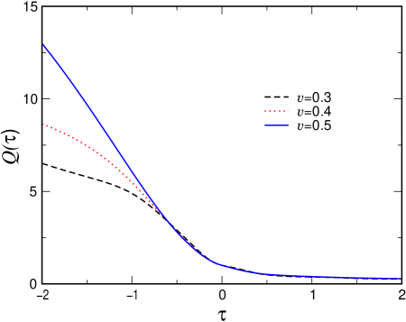
Figure 3: Elongation of bonds on the crack surface, $Q(\tau)$ for $\eta=0.5$.

We now proceed as before to change variables to $w$ and re-write this expression in terms of the auxiliary variable $\xi$ defined in Eq. (34a).

$$\det{\bf M}_{1}=-\frac{N(q)H(\xi)}{1+i\eta vq}+\hbox{term odd in $s$}$$ (53)

where

$$H(\xi) = \frac{3}{2}(1-e^{i\frac{q}{2}})(1+i\eta vq+\xi)(1+i\eta vq-\xi\cos\frac{q}{2}-\frac{v^{2}q^{2}}{3})$$ (54)

$$-\frac{3i}{2}\sin\frac{q}{2}(1+e^{i\frac{q}{2}})(\xi^{2}-(1+i\eta vq)^{2})$$

As before, the integrand in (52) has three poles. Dropping the irrelevant odd term and performing the integral leads to the expression

$$Q_{h}(q)=\frac{N(q)}{1+i\eta vq}(1-e^{-iq})\psi_{h}(q)$$ (55)

with

$$\psi_{h}(q)=\frac{1-e^{i\frac{q}{2}}}{2}-\frac{H(\xi_{1})\sqrt{\xi_{2}^{2}-(1+i\eta vq)^{2}}-H(\xi_{2})\sqrt{\xi_{1}^{2}-(1+i\eta vq)^{2}}}{3(\xi_{1}-\xi_{2})\sqrt{\xi_{1}^{2}-(1+i\eta vq)^{2}}\sqrt{\xi_{2}^{2}-(1+i\eta vq)^{2}}}\ .$$ (56)

Branches of the square root satisfy the same conditions (43), (44), as earlier. The function $N(q)$ can be found from Eq. (41)

$$N(q)=\frac{(1+i\eta vq)Q^{F}(q)}{1-S}\ .$$ (57)

Our final answer is

$$Q_{h}(q)=\frac{Q(0)}{\left.S^{+}\right|_{q=\frac{i}{\eta v}}S^{-}}\frac{(1-e^{-iq})\psi_{h}(q)}{(iq+0)(1+iq\eta v)}\ .$$ (58)

For $q$ close to $0$, the function $(1-e^{-iq})\psi_{h}(q)$ behaves as $q$, giving a divergence $1/q^{1/2}$ for $Q_{h}(q)$. This is similar to the divergence in $Q^{+}(q)$. Thus, the numerical calculation of $Q_{h}(\tau)$ is similar to the calculation of $Q(\tau)$ for $\tau>0$. Figure 4 displays $Q_{h}(\tau)$ for several values of $\eta$ and $v$. Generally speaking, the function $Q_{h}(\tau)$ has maxima in two different places, one somewhere in the vicinity of $-1$ and a second for $\tau>0$.

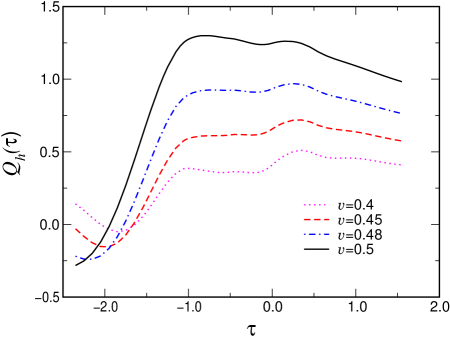
Figure 4: Elongation of the horizontal bonds, $Q_{h}(\tau)$, for $\eta=0.1$

We also need to find the bond elongation between the layers with $n=1$ and $n=2$ and between the layers with $n=-1$ and $n=0$. Due to the symmetry (31) it is sufficient to consider only $Q^{F}_{2}(q,n=\pm 1)$, which we will denote as $Q_{\pm}(q)$. We can derive for it an expression similar to that in Eq. (38) with the major difference being that in this case the odd parts of the explicit determinant in Eq. (32) do not cancel out because of the additional factor $w^{\pm 1}$.

$$Q_{\pm}(q) = \frac{N(q)}{2\pi i}\oint\limits_{|w|=1}w^{\pm 1}\frac{\frac{F(\xi)}{1+i\eta vq}+G(w)}{3\xi^{2}+\alpha\xi+\beta}\frac{dw}{w}$$ (59)

$$= \frac{N(q)}{2\pi i}\oint\limits_{|w|=1}\frac{\frac{F(\xi)}{1+i\eta vq}\pm G(w)}{3\xi^{2}+\alpha\xi+\beta}\,dw\ .$$

To derive the second equality, we used a change of variables $w\rightarrow 1/w$, along with the symmetries of $F$ and $G$. Again the integration in (59) is in the counter-clockwise direction. In this case, the integrand in the second form of the integral has just two poles inside the unit sphere, at $w_{1,2}$. After the by now familiar tedious calculations, we find

$$Q_{\pm}(q)=\frac{N(q)}{1+i\eta vq}\psi_{\pm}(q)$$ (60)

where

$$\psi_{\pm}(q)=-\frac{F(\xi_{1})w_{1}}{3(\xi_{1}-\xi_{2})\sqrt{\xi_{1}^{2}-(1+i\eta vq)^{2}}}+\frac{F(\xi_{2})w_{2}}{3(\xi_{1}-\xi_{2})\sqrt{\xi_{2}^{2}-(1+i\eta vq)^{2}}}$$

$$\pm\frac{g(q)(w_{1}-w_{2})}{3(\xi_{1}-\xi_{2})}$$ (61)

with

$$g(q)=-2i\sin\frac{q}{2}(v^{2}q^{2}-3(1+iq\eta v)\sin^{2}\frac{q}{2})$$ (62)

and $N(q)$ is again given by (57). Finally we obtain

$$Q_{\pm}(q)=\frac{Q(0)}{\left.S^{+}\right|_{q=\frac{i}{\eta v}}S^{-}}\frac{\psi_{\pm}(q)}{(iq+0)(1+iq\eta v)}$$ (63)

Just as was the case for $Q_{h}(q)$ and $Q^{+}(q)$, $Q_{\pm}(q)$ behaves as $1/q^{1/2}$ near $0$. Thus numerical calculations can be performed just as in the previous cases. Figure 5 shows several curves $Q_{\pm}(\tau)$ for differing parameters.

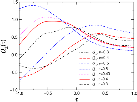
Figure 5: Elongation of bonds on the layer next to the crack layer, $Q_{\pm}(\tau)$ for $\eta=0.1$

Given the elongations of these “vulnerable” bonds, we can investigate the critical speed at which one of these bonds should be broken. Figure 6 shows the results of our calculations of this critical speed. In Figure 7 we plotted $\tau_{cr}$ at which these bonds break; this will allow us to identify spatial and time coordinates of braking and make contact with our finite lattice calculations later. We found that the maximum value of $Q_{-}(\tau)$ always reaches 1 before $Q_{+}(\tau)$ and that this is the most dangerous bond for small dissipation. This curve turns around at an $\eta$ of around $1.2$, so that $Q_{-}(\tau)$ is always subcritical for larger $\eta$. This is a result of the fact that the maximum value of $Q_{-}(\tau)$ is, surprisingly enough, not monotonic with velocity, but reaches a maximum and then decreases with increasing velocity. The maximum extension of this type of bond occurs, for large velocity, at some distance from the crack surface. For small $\eta$, where the maximum $Q_{-}(\tau)$ does exceed critical extension, the decrease of the maximum $Q_{-}$ with $v$ restabilizes the bond beyond some velocity. The dominant threshold for $\eta$ above about $1.1$, then, comes from the horizontal bond breaking. Note that as $\eta$ increases, the critical velocity decreases. Also, for small $\eta$, a crossover occurs as the relative importance of the two different maxima in the horizontal bond elongation reverse; this region is anyway irrelevant as the next-layer vertical bond breaks at a lower velocity. Whenever the horizontal bond dominates, the maximum at $\tau\simeq-1$ is the governing one. As we see from Figure 7 even for large $\eta$ this critical $\tau$ stays near $-1$, what means that horizontal bond always breaks near the tip of the crack, contrary to the Mode III case, where the point of breaking drifts backward with increasing $\eta$.

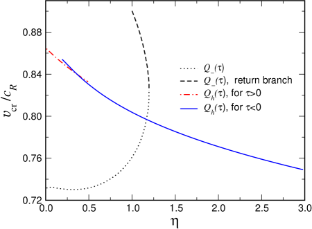
Figure 6: Critical speed $v_{\text{c}r}$

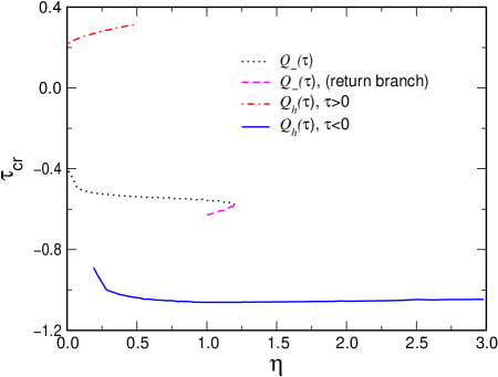
Figure 7: Time of bond breaking at critical speed

Many of these features are special to the Mode I problem, and have no analog in the Mode III calculation. For Mode III, the horizontal bond breaking always dominates. Furthermore, the maximum off-crack surface bond extension is a strictly increasing function of the velocity. This points to the possibility that the dynamics of Mode I may be much richer than the Mode III dynamics.

V Finite lattice model.

For our mode III calculations, it proved interesting to compare the exact results derived for an infinite lattice with the numerical determination of crack propagation properties in lattices of small transverse size (Kessler and Levine, 1998; Kessler, 2000). We now discuss similar calculations for our mode I model. In addition to providing details regarding the size needed to attain answers relevant to the macroscopic limit (a question of direct relevance for direct molecular dynamics simulations (Abraham, et al., 1994; Zhou, et al, 1997; Gumbsch, et al., 1997; Holland and Marder, 1997, 1998; Omeltchenko, et al., 1997), for example), finite lattice results can be used as a rough check on some of the predictions obtained above. Given the complexity of the analysis, having such a check is quite useful.

V.1 Arrested crack

Let us start with trying to find arrested cracks, expected to exist in some range of the driving $\Delta$ around the Griffith’s displacement. This involves looking for a solution of Eq. (1) with $\vec{u}(x,y)$ independent of time and with the forces on the right hand side arising solely from the broken bonds. If we have a system with a finite number of rows, the natural boundary condition requires that the top and bottom rows have fixed vertical displacements of $\Delta$ and $-\Delta$ respectively. Since the entire system is linear, we can choose to use $\Delta=1$ and rescale the breaking criterion accordingly.

Since we are doing a numerical calculation, we must introduce artificial boundaries in the direction along the crack, $\hat{x}$. What we do is cut off the range of points whose coordinates are variables and outside of this range impose fixed asymptotic displacements. On the cracked side, these are just $\vec{u}=\pm\Delta\hat{y}$ for positive and negative $y$. For the uncracked side, the asymptotic displacement involves constant strain. At each of the sites that has a variable displacement, we impose the two components of the (vectorial) equation of motion. We also impose the equations of motion at the boundaries of the system. This gives us more equations than we have variables. The coupling of sites which contain variable displacements with the ones with fixed displacements gives rise to inhomogeneous terms. Combining these observations, we can write our system in the schematic form $Mu-b=0$, with a non-square matrix $M$. The field $u$ is then determined by the requirement that the error be minimal. In this manner, the small errors introduced at the boundary by having to have a fixed box size are prevented from causing any large errors (by modes which grow exponentially away from the edges) in the bulk of the lattice.

The solution of this linear system determines the elongation of all bonds. In Figure 8 we show a typical lattice given by this solution. In fact we need to know elongation of just two bonds right at the tip of the crack; the one which in the case of the moving crack would break next ($Q_{n}$) and the other which would have been the last one broken ($Q_{l}$). Now, recall that we have scaled our displacement to equal unity and the only remaining displacement scale is the elongation at which the springs break, which we can call $\epsilon$. The solution we have found is consistent as long as $\epsilon$ is between the lower limit set by the $Q_{n}$ and the upper limit set by $Q_{l}$. Since $\Delta_{G}=\epsilon\sqrt{(2N+1)/3}$, where $2N$ is the number of rows in the $y$-direction (excluding the boundary rows whose displacement is constrained), we directly obtain the upper and lower limits of the arrested crack band

$$\frac{1}{\sqrt{\frac{1}{3}(2N+1)}Q_{l}}\ \leq\ \Delta/\Delta_{G}\ \leq\ \frac{1}{\sqrt{\frac{1}{3}(2N+1)}Q_{n}}$$ (64)

The results for these thresholds as a function of lattice size are shown in Figs. 9, 10. In the limit of infinite lattice, the lower limiting value $\Delta_{-}/\Delta_{G}$ approaches $0.515$, while the upper limiting value $\Delta_{+}/\Delta_{G}$ approaches $1.94$.

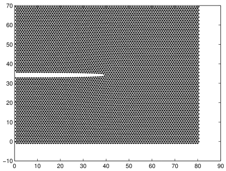
Figure 8: Finite size model for arrested crack.

Figure 9: Mode I on triangular lattice. Upper limiting $\Delta$ for arrested crack. Calculations were done for lattices with sizes $2m\times 2m$.

Figure 10: Mode I on triangular lattice. Lower limiting $\Delta$ for arrested crack. Calculations were done for lattices with sizes $2m\times 2m$.

V.2 Stable moving cracks

We now turn to the moving crack problem. Again, we need to solve Eq. (1) with the forces in the right part due to the broken bonds. Now, the displacement field $\vec{u}(x,y,t)$ is of course time dependent. Therefore, we need to introduce a time-step $\Delta t$ so as to define the time-points at which we will obtain a numerical solution. Given some specific speed $v$ of the crack, we choose to divide half of the time interval that it takes for the crack to propagate one lattice spacing, $1/(2v)$, into $n$ equal time intervals; thus $\Delta t=1/(2vn)$. Now we can discretize our system, obtaining equations at times $t=0,\Delta t,...,(n-1)\Delta t$. We use a symmetric discretization of first and second derivatives $(\vec{u}(t+\Delta t)-\vec{u}(t-\Delta t))/(2\Delta t)$ and $(\vec{u}(t+\Delta t)+\vec{u}(t-\Delta t)-2\vec{u}(t))/\Delta t^{2}$ correspondingly. These equations depend on displacements $\vec{u}$ outside of this time interval, because of the temporal derivatives. These can be found via use of the assumed symmetries of the moving crack; in fact, it is easy to see that we thereby trade in displacements outside of the modeled interval with displacements inside this interval albeit at a different spatial location. The boundaries are treated the same way as described for the arrested crack; the displacements outside some range are replaced by asymptotic values for all of the time-points in our interval. Including the equations at these boundary points again gives us a system in which the number of equations exceeds the number of variables and again a least squared error algorithm is used to find the required solution. Fig. 11 shows a snapshot of the lattice near the tip of the crack at one particular time for one set of parameters.

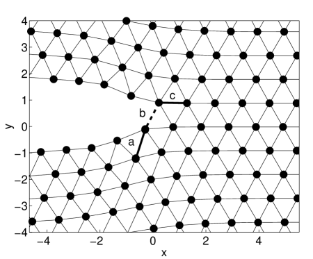
Figure 11: Snapshot of the region around tip of the crack for finite size model $2N\times 2N$ for moving crack with v=0.48, $\eta=1$, $n=5$, $N=24$.

We used these finite lattice calculations to provide an independent check on our analytic infinite lattice results. We were specifically interested in checking the critical speed estimates. The difficulty is that convergence in the parameter $1/N$ is fairly slow; and, using large lattices is rather time-consuming and memory-demanding. In practice, we limited our calculations to $N$’s ranging from $6$ to $24$. It turns out that for small dissipation where the next-row vertical bond vulnerability is the thing which determines the critical velocity, we can do a credible job of verifying that the infinite lattice results are consistent with the finite lattice ones. For example, in Fig. 12, we show the critical speed as a function of lattice size for several different values of $\eta$. These numbers, if extrapolated to infinite $N$ are clearly consistent with the results given earlier in Fig. 6, especially considering that having a finite time-step does introduce a small numerical error on its own. We can also check the critical time $\tau$ at which the bond breaking occurs. From Fig. (7), we see that in the infinite lattice the break occurs for $\tau\sim-0.5$. For the finite lattice with $n=5$, this mean that the bond $a$ highlighted in Fig. 11 should go above breaking threshold at the first time-point of the modeled interval. This is exactly what occurs.

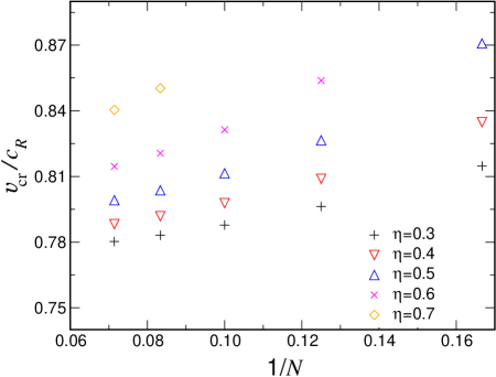
Figure 12: Critical speed due to the vertical bond braking on the layer next to the crack. $\diamond$  -$\eta=0.7$, $\times$ -$\eta=0.6$, $\triangle$ -$\eta=0.5$, $\bigtriangledown$ -$\eta=0.4$, $+$ -$\eta=0.3$

A different strategy is necessary for studying the onset of horizontal bond breaking. This is due to the fact that quite large $N$’s are required in order to for the results to quantitatively approach the infinite $N$ limit. This is another striking difference between the Mode I results and those of Mode III. For Mode III, the qualitative nature of the extraneous bond breaking was always similar to that of the infinite width limit, and the results were quantitatively accurate even for fairly small $N$’s. Here, however, the picture of which bonds are critical changes dramatically between finite $N$ and the infinite $N$ limit. In Fig. (13), we present the “phase diagram” for critical bonds for $N=38$, plotted together with the infinite $N$ result, and in Fig. (14), we compare the $N=38$ results to those for $N=26$. Since the steady-state code is difficult to run at these large values of $N$, the data in these two plots were obtained from time-dependent simulations, with only the central vertical bonds allowed to break. After running to times of $t=100$ to eliminate transients, the extensions of the dangerous bonds were checked to see if they exceeded criticality. Note that, in contradistinction to the “phase diagram” plotted in Fig. (6), we now plot $\Delta/\Delta_{G}$ on the vertical axis, since this is the input control parameter for the simulations. We see that qualitative behavior of the “$Q_{-}$” bonds is similar to the infinite-$N$ result, with these bonds being below critical extension for both large $\eta$ and large $\Delta/\Delta_{G}$. The horizontal bonds also behave qualitatively like their infinite-$N$ counterparts, but the quantitative agreement, is as we noted above, significantly worse. In fact, for large $\eta$, the most dangerous bond is in fact of “$Q_{+}$” type. However, the threshold at which the “$Q_{+}$” type bond becomes dominant is pushed to larger $\eta$ as the system size is increased, presumably going to infinity with $N$. Also, there is a small region of $\eta$ around 1.1 where the inconsistency is re-entrant, so that for intermediate values of $\Delta$, no bonds of the crack surface are critical. Thus, to see dynamics qualitatively representative of the macroscopic system requires very large system sizes at moderate to large $\eta$. Presumably, this is connected to the process zone increasing in size with $\eta$. Again, it is worth emphasizing that this is a feature not present in Mode III, and leads to the conclusion that in molecular dynamics simulations, the width of the material should be taken very large to accurately study the micro-branching instability.

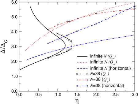
Figure 13: Comparison of the driving thresholds for critical bond extension for $N=\infty$ and $N=38$

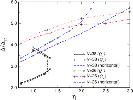
Figure 14: Comparison of the driving thresholds for critical bond extension for $N=38$ and $N=26$.

VI Discussion

In this work, we have discussed steady-state mode I crack propagation in a viscoelastic lattice model. Our primary method of analysis utilizes the Wiener-Hopf technique to write down closed form expressions for both the $v-\Delta$ curves (for various values of the dissipation $\eta$) and for the bond elongation field. The latter enables us to define a limit of consistency for the solution past which some bonds not along the crack path have elongations greater than the assumed breaking criterion. These results are new, and correspond to non-trivial extensions of the work of Kulamekhtova (1984) on the dissipationless limit and the work of Marder and Gross (1995) on small lattices.

The most interesting results, in our opinion, concern the dependence of the critical velocity (where the aforementioned inconsistency sets in) on the amount of dissipation. For small dissipation, this threshold is relatively insensitive to $\eta$, as already suggested in direct numerical simulations. This threshold, occurring at roughly .73 of the Rayleigh speed is in some ways reminiscent of the Yoffe (1951) branching criterion which suggests that straight crack propagation will become unstable once the largest stress direction shifts away from being straight ahead. It is unfortunately hard to be more precise regarding this correspondence since the crack dynamics in our model is fundamentally tied to the lattice scale, not the macroscopic scale - in fact, the latter is completely invisible in the Slepyan approach aside from providing a driving force in the form of a stress intensity factor.

At larger $\eta$, the instability picture changes. Now, it is a horizontal bond breaking which signals the onset of more complex crack dynamics. Also, the threshold goes down with increasing dissipation. This was not the case for our mode III calculations. This instability has nothing to do with Yoffe, as it is strongly dissipation dependent and in any case is not associated with crack branching.

Much of the recent theoretical work on mode I cracks has been motivated by experiments which show clearly that instabilities limit the range of steady-state crack propagation. These instabilities introduce more complex spatio-temporal dynamics to the fracture process, causing additional dissipation and leaving behind a roughened crack surface. It has been tempting to associate these results with the onset of inconsistencies in lattice models, although the details of this correspondence remains uncertain. First, most of the experimental work has been carried out in amorphous materials, making the idea of an ordered lattice model somewhat suspect. Next, the instabilities seen experimentally typically occur at smaller speeds than the ones seen in lattice systems with small dissipation. Finally, the experiments seem to show a typical frequency for micro-branching which is not connected in any obvious way to dynamics at a lattice scale.

Notwithstanding all these issues, we remain optimistic that the study of this class of models will lead to insight into dynamic fracture. There are several intriguing possibilities that need to be investigated in the future. First, we have shown that for mode I cracks, increasing the dissipation (in the form of a Kelvin viscosity) eventually results in a decrease of the instability threshold. If our model is really applied at the atomic scale, it is hard to see why there should be a large linear dissipation; on the other hand, it is well-known that lattice models miss an essential non-linear dissipation mechanism, namely the creation of dislocations which remain pinned to the crack. Would inclusion of these effects also lower the threshold? On the other hand, applying the model on a large scale (possibly for a disordered system) would naturally require a large dissipation and recent numerical simulations indicate that proper inclusion of the thermal fluctuations might also push the model into better agreement with experiment (Pla, et al., 1998; Sander and Ghasias, 1999). Finally, the exact nature of the state which occurs past the instability onset has not been addressed in our work to date, and in fact cannot be addressed by the elegant but ultimately limiting analytic methods utilized for the steady-state problem. Instead, we plan to study a generalized force law in which the sharp breaking criterion is replaced by an analytic nonlinear force versus displacement (Kessler and Levine, 1999). In this formulation, the inconsistency found here becomes a linear instability of the steady-state crack (Kessler and Levine, 2000) and one can use some of the methods developed in the field of nonequilibrium pattern formation to unravel the dynamics past onset. These studies, together with additional experimental data regarding the differences between brittle fracture in crystalline versus non-crystalline materials, will hopefully lead to a better understanding of dynamic fracture.