Steady-state mode III cracks in a viscoelastic lattice model

Abstract

We extend the Slepyan solution of the problem of a steady-state crack in an infinite ideally brittle lattice model to include dissipation in the form of Kelvin viscosity. As a demonstration of this technique, based on the Wiener-Hopf method, we apply the method to mode III cracks in a square lattice. We use this solution to find the critical velocity at which the steady-state solution becomes inconsistent due to additional bond-breaking; this point signaling the onset of complex dynamical behavior.

Keywords: Crack Propagation and Arrest, Dynamic Fracture, Crack Branching and Bifurcation

I Introduction

Recent experiments on dynamical fracture (Fineberg, et al., 1991, 1992) have shown that cracks in brittle materials become unstable above a critical velocity. This instability is associated with the formation of a roughened fracture surface, with an increased dissipation of elastic energy, and with complicated velocity dynamics - for a review, see (Fineberg and Marder, 1999). Although there are hints of such an instability in the traditional continuum formulations of ideally brittle cracks (Yoffe, 1951), a systematic treatment does not appear possible. Indeed, recent attempts (Langer and Lobkovsky, 1998) to utilize a cohesive stress modification (Barenblatt, 1959) of the continuum elastic equations in order to address this problem have been rather unsuccessful.

In the absence of a compelling continuum approach, one must deal in some manner with discrete dynamics on the “atomic scale”. In this regard, Slepyan (Slepyan, 1981, 1982; Kulamekhtova, 1984) pioneered the idea of studying lattice models in which atoms interact (via piece-wise linear springs) with their neighbors in a predetermined lattice geometry. This conceptual framework was further developed by Marder and collaborators (Marder and Gross, 1995; Marder and Liu, 1993). Here, one can directly obtain the relationship between the crack tip velocity and the imposed driving and furthermore one can search for conditions which do not allow stable steady crack motion. Clearly, lattice models are not fully realistic, especially at displacements that are not small compared to the underlying lattice spacing; to be more realistic, one must resort to molecular dynamics simulations including all possible atomic interactions (Abraham, et al., 1994; Zhou, et al., 1997; Gumbsch, et al., 1997; Holland and Marder, 1997, 1998; Omeltchenko, et al., 1997). However, the analytic tractability of these models as well as indications (Marder and Gross, 1995; Pla, et al., 1998; Sander and Ghasias, 1999) that they do contain the essential mechanism responsible for the observed dynamical instability make them well worthy of serious attention.

Slepyan recognized that in an ideally brittle material (where each spring is linear until a displacement at which it completely breaks) one can use Fourier methods to find the lattice analog of a traveling wave solution. In this solution, each point on the lattice (at the same transverse coordinate) undergoes the same time history of motion as any other, albeit with some time delay. Once one obtains the solution, one must check that all springs assumed to be linear have displacements that are in fact below the breaking threshold. The violation of this assumption by the steadily propagating solution signals the onset of more complex dynamical behavior, at least in qualitative accord to what is seen experimentally (Fineberg and Marder, 1999; Marder and Gross, 1995). Using the Wiener-Hopf technique, Slepyan solved for the velocity-driving curve in the limit where the width of the lattice transverse to the crack direction goes to infinity.

One important consideration in all models of brittle fracture concerns dissipation mechanisms. From our perspective, it makes sense to put in dissipation at the lattice scale in such a way so as not dominate the large-scale continuum elastic field. If in addition one demands an equation that is local in time, one is led (Langer, 1992; Pla, et al., 1998) to the introduction of a Kelvin viscosity which dissipates energy proportional to the rate of change of spring lengths. In the naive continuum limit, this gives rise to a third derivative (two space, one time) term. That means that if the viscosity is chosen to be O(1) on the lattice scale, it will scale to zero as far as the macroscopic dynamics is concerned. We saw this explicitly in a previous set of papers (Kessler and Levine, 1998; Kessler, 2000) which solved this problem for finite width lattices and considered the nature of the solution as the width became large. Nevertheless, the viscosity can have a considerable effect on aspects of the solution which depend on the microscopic details, namely the crack speed (for a fixed stress intensity factor) and the self-consistency of the traveling wave ansatz.

The rest of this paper is organized as follows. In the next section, we formally define the model, employing Slepyan’s idea (Slepyan, 1981; Kulamekhtova, 1984) of replacing the driving at some external boundary with some local forcing on the crack surface. This allows for the solution in Section III of the strictly infinite lattice model; the connection to a finite problem with some displacement driving is made by appealing to the universality of the microscopic crack solution given a fixed stress intensity factor. In the following section, we discuss the numerical evaluation of the velocity curve from its formal expression. Following that, we turn to the aforementioned self-consistency condition and study the effect of dissipation on the critical velocity. We conclude with some observations in the final section.

II Square lattice model

We wish to study mode III cracks and the effects thereupon of Kelvin viscosity. Our model thus consists of a square lattice of mass points undergoing (scalar) displacements out of the plane. The lattice extends infinitely long in both the $x$ (along-crack) and $y$ (transverse) directions. The lattice points are connected to their nearest neighbors by ideally brittle springs which behave linearly with spring constant 1 until some threshold elongation $2\epsilon$ at which point they irreversibly crack. All the (uncracked) springs have a viscous damping $\eta$. Let us assume that the crack corresponds to a sequential breaking of the vertical bonds between the mass points at rows $y=1$ and $y=0$. The equation of motion for the masses in rows $y>1$ reads

$${\ddot{u}}(x,y)=\left(1+\eta\frac{d}{dt}\right)\Big{(}u(x+1,y)+u(x-1,y)+u(x,y+1)+u(x,y-1)-4u(x,y)\Big{)}\ .$$ (1)

We allow the vertical bonds along the crack surface to have a different spring constant $k$ and damping parameter $\tilde{\eta}$, to model the effect of having weak links along the crack surface. The equation for $y=1$ then reads, using the assumed symmetry $u(x,y)=-u(x,1-y)$,

$${\ddot{u}}(x,y) = \left(1+\eta\frac{\partial}{\partial t}\right)\Big{(}u(x+1,1)+u(x-1,1)+u(x,2)-3u(x,1)\Big{)}$$ (2)

$$\quad+\theta(\epsilon-u(x,1))\left(k+\tilde{\eta}\frac{\partial}{\partial t}\right)\Big{(}-2u(x,1)\Big{)}\ .$$

It is easily verified that the equations for $y\leq 0$ are consistent with the above symmetry. We can, without loss of generality choose $\epsilon=1/2$ (so that the threshold elongation is unity). Note that in these units, the elastic wave speed is unity, so all velocities are dimensionless, expressed as fractions of the wave speed.

We are interested in steady-state cracks, described by the Slepyan traveling wave ansatz,

$$u(x,y,t)=u(x-vt,y)$$ (3)

which implies that every mass point in a given row undergoes the same time history, translated in time. We choose the origin of time such that $u(0,1)=\epsilon$, so that it represents the moment of cracking of the spring in column 0. If we define $\tau=x-vt$, the equations of motion for $y>1$ become

$$\left(1-\eta v\frac{\partial}{\partial\tau}\right)\Big{(}u(\tau+1,y) + u(\tau-1,y)+u(\tau,y-1)$$ (4)

$$+ u(\tau,y-1)-4u(\tau,y)\Big{)}-v^{2}\frac{\partial^{2}u(\tau,y)}{\partial\tau^{2}}\ =0\ .$$

For $y=1$, we separate out the terms proportional to $\theta(-\tau)$, giving

$$\left(1-\eta v\frac{\partial}{\partial\tau}\right)\Big{(}u(\tau+1,1)+u(\tau-1,1) + u(\tau,2)-3u(\tau,1)\Big{)}$$

$$+\left(k-\tilde{\eta}v\frac{\partial}{\partial\tau}\right)\Big{(}-2u(\tau,1)\Big{)} - v^{2}\frac{\partial^{2}u(\tau,1)}{\partial\tau^{2}}=-\sigma(\tau)\ .$$ (5)

The driving term for this equation has the form

$$\sigma(\tau)=\theta(-\tau)\left[F_{0}+2\left(k-\tilde{\eta}v\frac{\partial}{\partial\tau}\right)u(\tau,1)\right]\ .$$ (6)

In this expression, we have inserted an external force $F_{0}$ which acts on the crack boundaries. This force is an artifice which serves as an inhomogeneous source term, in place of introducing the driving through the boundary condition on the top and bottom surfaces. We will see later how to choose this function.

We Fourier transform with respect to $\tau$ (see the appendix for our conventions regarding Fourier transforms and Fourier integrals). If we assume that $u(q,y)=\chi_{q}[\xi(q)]^{y-1}$ for $y\geq 1$, we obtain from Eqn. (4) the dispersion relationship

$$(1+iq\eta v)(e^{-iq}+e^{iq}+\xi+\frac{1}{\xi}-4)+q^{2}v^{2}=0$$ (7)

This can be rewritten as

$$(\xi^{1/2}-\frac{1}{\xi^{1/2}})^{2}=4\sin^{2}\frac{q}{2}-\frac{q^{2}v^{2}}{1+iq\eta v}\equiv h^{2}$$ (8)

which therefore implies that $\xi^{1/2}=\pm h/2\pm\sqrt{(h/2)^{2}+1}$. If we define

$$r^{2}\equiv h^{2}+4$$

then we can write

$$\xi=\frac{(r-h)^{2}}{4}=1-\frac{h(h-r)}{2}=\frac{r-h}{r+h}$$ (9)

Note that we have must choose the sign that corresponds to a decaying solution in the $y$ direction, i.e. $|\xi|<1$.

If we substitute this ansatz into Eqn. (II), we get

$$\left(-2(k+iq\tilde{\eta}v)+(1+iq\eta v)(1-\frac{1}{\xi})\right)\chi=-\sigma^{F}$$ (10)

where $\sigma^{F}$ is the Fourier transform of $\sigma$. Noting that $-1-\frac{1}{\xi}=-\frac{r(r+h)}{2}$, we obtain

$$\chi_{q}=\frac{2\sigma^{F}}{N(q)}$$ (11)

with

$$N(q)=h(r+h)(1+i\eta vq)+4(k+i\tilde{\eta}vq)\ .$$ (12)

This equation is implicit, since the driving term $\sigma^{F}$ on the right hand side still depends on the displacement field $u(\tau,1)$. In the next section, we solve this equation via the Wiener-Hopf technique.

III Wiener-Hopf solution

Let us define $\vee(\tau)=2u(\tau,1)$, the bond elongation between rows $y=0$ and $y=1$. In the appendix, we define $\vee^{+}(q)$ and $\vee^{-}(q)$ as the decomposition of $\vee(\tau)$ into terms which are analytic in the upper and lower half planes respectively. This allows us to write Eq. (6) as

$$\sigma^{F}(q)=F_{0}^{-}(q)+(k+i\tilde{\eta}vq)\vee^{-}(q)-\tilde{\eta}v\vee(0)$$ (13)

where we have employed a similar breakup for the driving term $F_{0}$, and where we have utilized Eq. (62).

Substituting the formula for $\sigma^{F}$ into Eqn. (10) for $\chi=(\vee^{+}+\vee^{-})/2$ leads to a closed form equation for $\vee$; namely

$$\vee^{+}+\vee^{-}(1-\frac{4(k+i\tilde{\eta}vq)}{N(q)})=\frac{4F_{0}^{-}}{N(q)}-\frac{4\tilde{\eta}v\vee(0)}{N(q)}\ .$$ (14)

Defining $S$ by

$$S\equiv 1-\frac{4(k+i\tilde{\eta}vq)}{N(q)}=\frac{h(1+i\eta vq)}{h(1+i\eta vq)+(r-h)(k+i\tilde{\eta}vq)}\ ,$$ (15)

we can rewrite Eq. (14) as

$$\vee^{+}+S\vee^{-}+\frac{\tilde{\eta}v}{k+iq\tilde{\eta}v}(1-S)\vee(0)=\frac{(1-S)F_{0}^{-}}{k+iq\tilde{\eta}v}\ .$$ (16)

We will solve this equation using the Wiener-Hopf technique. The key is to factor $S$ into a product of two pieces, $S(q)=S^{+}(q)S^{-}(q)$, each of which is regular in the upper ($S^{+}$) or lower ($S^{-}$) half plane. Doing so, we get

$$\frac{\vee^{+}}{S^{+}}+S^{-}\vee^{-}+\frac{\eta v}{k+iq\tilde{\eta}v}\left(\frac{1}{S^{+}}-S^{-}\right)\vee(0)=\frac{1-S}{S^{+}}\frac{F_{0}^{-}}{k+iq\tilde{\eta}v}\ .$$ (17)

We then have to deal with the extra singularity at $q=\frac{ik}{\eta v}$. We do this by a simple subtraction

$$\frac{\vee^{+}}{S^{+}}+S^{-}\vee^{-}+\frac{\tilde{\eta}v\vee(0)}{k+iq\tilde{\eta}v}\left(\frac{1}{S^{+}}-\left.\frac{1}{S^{+}}\right|_{q=\frac{ik}{\tilde{\eta}v}}+\left.\frac{1}{S^{+}}\right|_{q=\frac{ik}{\tilde{\eta}v}}-S^{-}\right)\ =\ \frac{1-S}{S^{+}}\frac{F_{0}^{-}}{k+iq\tilde{\eta}v}\ .$$ (18)

We have now to choose $F_{0}$, our external forcing. In taking the width to infinity, in essence we are solving for the “inner” solution in the sense of boundary-layer theory; i.e., only on the scale of the lattice spacing. The external forcing in the finite width problem only acts on the large scale, and does not vary on the lattice scale. Thus, $F_{0}$ must have support only at $q=0$. Following Slepyan, then, we choose $F_{0}$ such that

$$\frac{1-S}{S^{+}(k+iq\tilde{\eta}v)}F_{0}^{-}=2\pi B\delta(q)=B\left(\frac{1}{iq+0}+\frac{1}{-iq+0}\right)\ ,$$ (19)

where $B$ is a constant. This then gives us the the two separate equations

$$\vee^{+} = -\frac{{\tilde{\eta}}v\vee(0)}{k+iq\tilde{\eta}v}\left(1-\frac{S^{+}}{S^{+}|_{q=\frac{ik}{\tilde{\eta}v}}}\right)+\frac{BS^{+}}{-iq+0}\ ,$$ (20a)

$$\vee^{-} = -\frac{\tilde{\eta}v\vee(0)}{k+iq\tilde{\eta}v}\left(\frac{1}{S^{-}S^{+}|_{q=\frac{ik}{\eta v}}}-1\right)+\frac{B}{(iq+0)S^{-}}\ .$$ (20b)

As shown in Eqs. (59) and (61) we can solve for $\vee(0)$ from Eqs. (20a) or (20b) by multiplying the first by $-iq\rightarrow+\infty$ or the second by $iq\rightarrow+\infty$. This yields

$$\vee(0)=B\left.S^{+}\right|_{q=\frac{ik}{\tilde{\eta}v}}\ .$$ (21)

Substituting this back into Eqns. (20), and defining $\eta_{k}\equiv{\tilde{\eta}}/k$, we find

$$\vee^{+} = \frac{BS^{+}}{(-iq+0)(1+iq\eta_{k}v)}-\frac{\eta_{k}vB}{1+iq\eta_{k}v}\left.S^{+}\right|_{q=\frac{i}{\eta_{k}v}}\ ,$$ (22a)

$$\vee^{-} = \frac{B}{(iq+0)(1+iq\eta_{k}v)S^{-}}+\frac{\eta_{k}vB}{1+iq\eta_{k}v}\left.S^{+}\right|_{q=\frac{i}{\eta_{k}v}}S^{-}$$ (22b)

These equations directly determine the displacements given the strength of the external driving, $B$. To get a physical handle on the meaning of this constant, we note that Eqns. (20) can be directly solved for the leading behavior of $\vee^{\pm}$ as $q$ goes to $0$, using the fact that in this limit,

$$S^{\pm}\sim\kappa^{\pm 1}\sqrt{A}(q\pm i0)^{1/2}$$ (23)

where $A=\frac{\sqrt{1-v^{2}}}{2k}$, and $\kappa$ is a constant, reflecting the arbitrariness in how we perform the decomposition of $S$. We find

$$\vee_{+}\sim\kappa\sqrt{A}\frac{i^{1/2}B}{(-iq+0)^{1/2}}$$ (24a)

$$\vee_{-}\sim\frac{\kappa}{\sqrt{A}}\frac{i^{1/2}B}{(iq+0)^{3/2}}$$ (24b)

This is just the expected (Fourier transform of) the singular solution of continuum elasticity as one approaches the crack tip. Thus, as in all boundary-layer problems, the large-distance limit of the “inner” solution matches on to the short-distance limit of the “outer” solution, confirming the justification of the choice of $F_{0}$ above. We need to relate the strength of the short-distance singularity of the continuum solution to the driving displacement $\Delta$. This can be done directly by solving the continuum elastic equations. It is easier, however, to follow Slepyan and derive this relation by energy considerations. One can calculate (Slepyan, 1981) the flux of energy into the boundary-layer, or “process” zone, obtaining

$$T=\frac{ik\kappa^{2}B^{2}}{2}v$$ (25)

Now consider the flux of energy $T_{0}$ being used to break bonds, which is simply related to $\vee(0)$

$$T_{0}=\frac{k\left(B\left.S^{+}\right|_{q=\frac{i}{\eta_{k}v}}\right)^{2}}{2}v\ .$$ (26)

Then, using the idea that the Griffith’s displacement is determined by exactly the condition that all the energy flux is needed just to break the bonds, we have

$$\frac{\Delta}{\Delta_{G}}=\sqrt{\frac{T}{T_{0}}}=\frac{i^{1/2}\kappa}{\left.S^{+}\right|_{q=\frac{i}{\eta_{k}v}}}$$ (27)

Notice that the factor of $\kappa$ guarantees that the result is invariant with respect to how the decomposition of $S$ is performed.

In order to make contact with other treatments, we consider the standard case $k=1$ and $\eta_{k}=\tilde{\eta}=\eta$, in which all bonds are equivalent. In this case, the function $S$ has a particularly simple form,

$$S(q)=\frac{h}{r}=\frac{H}{R}$$ (28)

with $H^{2}=4(1+iq\eta v)\sin^{2}\frac{q}{2}-q^{2}v^{2}$ and $R^{2}=4(1+iq\eta v)(\sin^{2}\frac{q}{2}+1)-q^{2}v^{2}$. We can represent these functions in term of the products over all their roots

$$H = \sqrt{1-v^{2}}(q+i0)^{1/2}(q-i0)^{1/2}\prod_{n,m}\left(1-\frac{q}{Q^{+}_{n}}\right)^{1/2}\left(1-\frac{q}{Q^{-}_{m}}\right)^{1/2}$$ (29)

$$R = 2\prod_{n,m}\left(1-\frac{q}{q^{+}_{n}}\right)^{1/2}\left(1-\frac{q}{q^{-}_{m}}\right)^{1/2}$$ (30)

where $Q^{+}_{n}(q^{+}_{n})$ are the (nonzero) roots of $H^{2}$($R^{2}$) in the lower half plane and $Q^{-}_{n}(q^{-}_{n})$ are corresponding roots of $H^{2}$($R^{2}$) in the upper half plane. This decomposition allows us to write down explicitly the factors $S^{+}$, $S^{-}$:

$$S^{+}(q)=\frac{(1-v^{2})^{1/4}}{\sqrt{2}}(q+i0)^{1/2}\prod_{n,m}\left(\frac{1-\frac{q}{Q^{+}_{n}}}{1-\frac{q}{q^{+}_{m}}}\right)^{1/2}$$ (31a)

$$S^{-}(q)=\frac{(1-v^{2})^{1/4}}{\sqrt{2}}(q-i0)^{1/2}\prod_{n,m}\left(\frac{1-\frac{q}{Q^{-}_{n}}}{1-\frac{q}{q^{-}_{m}}}\right)^{1/2}$$ (31b)

Examining the small $q$ behavior, we find the $\kappa=1$, so that substitution of $S^{+}$ into Eqn. (27) gives

$$\frac{\Delta}{\Delta_{G}}=\frac{(2\eta v)^{1/2}}{(1-v^{2})^{1/4}}\prod_{n,m}\left(\frac{1-\frac{i}{\eta vq_{n}^{+}}}{1-\frac{i}{\eta vQ_{m}^{+}}}\right)^{1/2}$$ (32)

If we explicitly take out of the product in Eq. (32) the one imaginary $q^{+}$, which we will denote as $q^{+}_{0}$, we get

$$\frac{\Delta}{\Delta_{G}}=\frac{1}{(1-v^{2})^{1/4}}\sqrt{\frac{2(1+iv\eta q^{+}_{0})}{iq^{+}_{0}}}\prod_{n\neq 0,m}\left(\frac{1+iv\eta q^{+}_{n}}{1+iv\eta Q^{+}_{m}}\frac{Q^{+}_{m}}{q^{+}_{n}}\right)^{1/2}$$ (33)

This formula was obtained by Kessler (2000), who started from a finite lattice of transverse size $N_{y}$ and considered the $N_{y}\rightarrow\infty$ limit. Note that this can be done for $k=1$ on a square lattice, (the case being considered here), but not for general $k$ or for modes I or III on a triangular lattice; the method here works for these cases as well (Pechenik, et al., 2000).

Next, it is easy to see that in the limit $\eta\rightarrow 0^{+}$, we have $\left.S\right|_{q=\frac{i}{\eta v}}=1$ and that therefore

$$\frac{\Delta}{\Delta_{G}}=\left(i\left.\frac{S^{-}}{S^{+}}\right|_{q=\frac{i}{\eta v}}\right)^{1/2}=i^{1/2}\prod_{n,m}\left(\frac{q^{-}_{m}Q^{+}_{n}}{q^{+}_{m}Q^{-}_{n}}\right)^{1/4}\ .$$ (34)

Furthermore, in this limit $q^{+}_{0}=-q^{-}_{0}$. All other complex roots cancel out, leaving only real roots. Hence,

$$\frac{\Delta}{\Delta_{G}}=\prod_{over\>real\>Q_{n},\,q_{m}}\left(\frac{q^{-}_{m}Q^{+}_{n}}{q^{+}_{m}Q^{-}_{n}}\right)^{1/4}\ ,$$ (35)

a result originally obtained by Slepyan. Note that in our treatment, the presence of one of these real roots in either the numerator or the denominator of the product expression depends entirely on the half-plane from where it came as we took the limit $\eta\rightarrow 0^{+}$. To see what this condition implies, let us denote by $H^{2}$(or $R^{2}$) as $f$; then the small imaginary part of a specific real root, $i\delta$, satisfies the equation

$$\left.i\delta\frac{\partial f}{\partial q}\right|_{\eta=0,\;q=q_{real}}+\eta\left.\frac{\partial f}{\partial\eta}\right|_{\eta=0,\;q=q_{real}}=0\ ,$$ (36)

which gives as the determining factor

$${\delta\over\eta}=\left.\frac{-q^{3}v^{3}}{\frac{\partial}{\partial q}(4\sin^{2}\frac{q}{2}-v^{2}q^{2})}\right|_{q=q_{real}}\ .$$ (37)

This condition is exactly what appears in Slepyan’s work.

IV Numerical calculations

In this section we derive an integral form for the basic result Eq. (32). We then present a numerical procedure for finding the displacement-velocity curve. The basic notion is to utilize Eq. (VII) to find $S^{+}$. It is more convenient for the numerical work to isolate explicitly the singularity at $q=0$, defining $K(q)$ by

$$S^{2}(q)=\frac{A^{2}\phi^{2}(q+i0)(q-i0)}{q^{2}+\phi^{2}}K(q)$$ (38)

where $\phi$ is an arbitrary positive constant. Because of the factor $A^{2}q^{2}$ in the denominator, $K(0)=1$; the factor $(q^{2}+\phi^{2})/\phi^{2}$ does not alter the desired asymptotic behavior at infinity: $K\rightarrow const$ as $q\rightarrow\pm\infty$. Applying Eq. (VII), we get for $Im\;q>0$

$$S^{+}=\exp{\frac{1}{4\pi i}\int_{-\infty}^{+\infty}\frac{\ln S^{2}(\gamma)}{\gamma-q}d\gamma}=\left(A\phi\frac{q+i0}{q+i\phi}\right)^{\frac{1}{2}}\left(K^{+}\right)^{\frac{1}{2}}$$ (39)

and for $Im\;q<0$

$$\frac{1}{S^{-}}=\exp{\frac{1}{4\pi i}\int_{-\infty}^{+\infty}\frac{\ln S^{2}(\gamma)}{\gamma-q}d\gamma}=\left(\frac{1}{A\phi}\frac{q-i\phi}{q-i0}\right)^{\frac{1}{2}}\left(K^{-}\right)^{-\frac{1}{2}}$$ (40)

with

$$\left(K^{\pm}\right)^{\pm\frac{1}{2}}=\exp{\frac{1}{4\pi i}\int_{-\infty}^{+\infty}\frac{\ln K(\gamma)}{\gamma-q}d\gamma}$$ (41)

where the upper sign is for $Im\;q>0$ and the lower sign for $Im\;q<0$.

There is one point regarding these expressions that must be clarified. We must make the correct choice of the branch cuts for the square roots in $h$ and $r$ appearing in $S$. It is convenient to express things in terms of $S^{*}(q)\equiv h/r=H/R$, the simple $k=1$ and $\eta_{k}=\eta$, form of $S$, so that from Eqn. (15)

$$S=\frac{S^{*}(1+i\eta vq)}{S^{*}(1+i\eta vq)+(1-S^{*})k(1+i\eta_{k}vq)}\ ,$$ (42)

and from Eqn. (9)

$$\xi=\frac{1-S^{*}}{1+S^{*}}\ .$$ (43)

We must choose $S^{*}$ such that $|\xi|<1$ as noted below Eqn. (9). It is easy to see from the above expression for $\xi$ that it is sufficient to choose $S^{*}$ to lie in the first and fourth quadrants to guarantee this. For $S^{*}$, we can then generate $S$ directly via Eqn. (42), and from this $K$.

As $K(0)=1$, there is no pole in the integral (41) at $\gamma=0$ when $q=0$. This means that $K^{+}(0)=(K^{-}(0))^{-1}$ and the asymptotic expressions for $S^{\pm}$ are

$$S^{+}|_{q\rightarrow 0}=\sqrt{\frac{AK^{+}(0)}{i}}(q+i0)^{\frac{1}{2}};\;\;\;S^{-}|_{q\rightarrow 0}=\sqrt{\frac{iA}{K^{+}(0)}}(q-i0)^{\frac{1}{2}}\ .$$ (44)

Comparing this to Eqn. (23), we have

$$\kappa=\sqrt{-iK^{+}(0)}\ ,$$ (45)

so that

$$\frac{\Delta}{\Delta_{G}}=\sqrt{\frac{1+\phi\eta_{k}v}{A\phi}\frac{K^{+}(0)}{K^{+}(\frac{i}{\eta_{k}v})}}$$ (46)

Explicitly writing out the integrals, we get

$$\frac{\Delta}{\Delta_{G}}=\sqrt{\frac{1+\phi\eta_{k}v}{A\phi}}\exp{\frac{1}{4\pi i}\int_{-\infty}^{+\infty}\frac{\ln K(\gamma)}{\gamma(1+i\eta_{k}v\gamma)}d\gamma}$$ (47)

The extra degree of convergence of the integrand at infinity is very desirable, as it helps control the fact that $\ln K(\xi)$ is a rapidly oscillating function. Also, the fact that the answer must be independent of $\phi$ provides a check on the numerical routines. A change of variables $\gamma\rightarrow-\gamma$ allows the integral to be rewritten as

$$\frac{\Delta}{\Delta_{G}}=\sqrt{\frac{1+\phi\eta_{k}v}{A\phi}}\exp{\frac{1}{4\pi}\int_{0}^{+\infty}Im\frac{\ln K(\gamma)}{\gamma(1+i\eta_{k}v\gamma)}d\gamma}$$ (48)

To actually compute this integral, we divided the region of integration into two parts from $0$ to $1$ and from $1$ to $+\infty$. The second integral was further transformed so as to have in the numerator the factor $\ln A^{2}\phi^{2}K(\xi)$ which goes to zero at infinity; the subtracted integral with the numerator $\ln 1/(A\phi)^{2}$ was performed analytically. After all these manipulations, the integrals were successfully computed by standard mathematical library subroutines.

Results from our numerical calculations for $k=1$ and $\eta_{k}=\tilde{\eta}=\eta$, are presented in Figs. 1, 2, which reproduce, of course, those of (Kessler, 2000). At small $\eta$, there are large oscillations in the $v$ vs $\Delta$ curve, as found initially by Marder and Gross for lattices with small transverse sizes. The curves all hit the $v=0$ line at the point which marks the end of the band of lattice-trapped static cracks (Kessler and Levine, 1998). For larger damping, the oscillations disappear and the moving crack branch bifurcates smoothly (in the backward direction) from this point, eventually turning around and becoming stable. In Fig. 3, we contrast the standard result to that for smaller $k$, keeping $\eta_{k}=\eta$. We see that the $v=0$ limit has moved closer to unity, in accord with the finding in (Kessler and Levine, 1998) that the window of arrested cracks narrows as $k$ decreases (note for purposes of comparison that our $k$ is a factor of 2 smaller than that defined in (Kessler and Levine, 1998). The velocity at the minimum $\Delta/\Delta_{G}$ however is hardly affected, so the minimum stable velocity is essentially unchanged. Past this point, the velocity is higher at smaller $k$, even when the change in $\Delta_{G}$ is factored in. This is further evidence of how the microscopic details influence the velocity versus driving displacement curve.

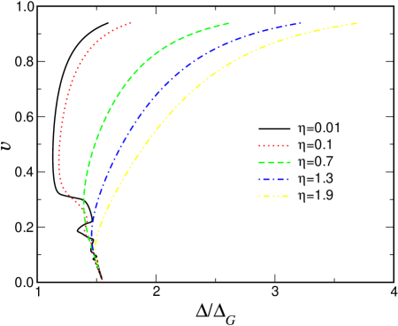
Figure 1: Dependence of speed $v$ on dimensionless driving $\frac{\Delta}{\Delta_{G}}$ for $k=1$ and $\eta_{k}=\eta$. The curves are for $\eta=0.01$, $0.1$, $0.7$, $1.3$, $1.9$

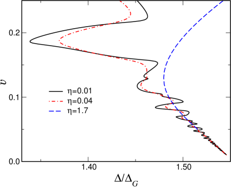
Figure 2: Change from rapid oscillations for small $\eta$ to smooth behavior at large $\eta$. Here $k=1$ and $\eta_{k}=\eta$.

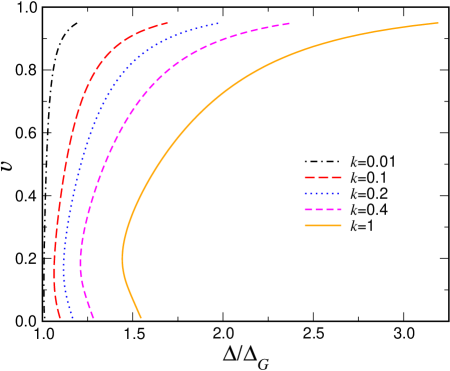
Figure 3: Dependence of speed $v$ on dimensionless driving $\Delta/\Delta_{G}$ for $k=0.01$, $0.1$, $0.2$, $0.4$, $1.0$. Here $\eta=\eta_{k}=1.1$

V Consistency of the solution

As mentioned in the introduction, cracks become unstable above a critical velocity. In the framework of the model being considered here, one might assume that this velocity is associated with the solution as found by the Wiener-Hopf method becoming inconsistent. As we shall see, there are two kinds of inconsistencies. The first sets in for small $v$, for small enough $\eta$. Here the vertical bond between $y=0$ and $y=1$ first achieves critical extension prematurely, at some positive $\tau$, contradicting the assumption that the bond breaks at $\tau=0$. In the second kind of inconsistency, a horizontal bond achieves critical extension. If the model is defined so that only the vertical bonds between $y=0$ and $y=1$ are breakable, then this does not present a problem. If one the other hand, all the springs are chosen identical, so that the horizontal springs also break at the same critical extension as the vertical ones, then the solution is indeed inconsistent at this point. This is what occurs at large enough velocity, for all $\eta$.

To proceed, we must calculate the bond lengths, back transforming our Fourier space solutions so as to obtain the physical displacements. We find the time dependence of the function $\vee(\tau)$. From Eqs. (20a), (20b) and (21), we have

$$\vee^{+}=\frac{\vee(0)}{(-iq+0)(1+iq\eta_{k}v)}\frac{S^{+}}{\left.S^{+}(q)\right|_{q=\frac{i}{\eta_{k}v}}}-\frac{\eta_{k}v\vee(0)}{1+iq\eta_{k}v}\ ;$$ (49)

$$\vee^{-}=\frac{\vee(0)}{\left.S^{+}\right|_{q=\frac{i}{\eta_{k}v}}S^{-}(q)}\frac{1}{(iq+0)(1+iq\eta_{k}v)}+\frac{\eta_{k}v\vee(0)}{1+iq\eta_{k}v}\ .$$ (50)

Performing the inverse Fourier transform, we get

$$\vee(\tau)=\vee(0)\int_{-\infty}^{+\infty}\frac{\sqrt{A\phi}e^{-iq\tau}}{\sqrt{(iq-0)(iq-\phi)}(1+iq\eta_{k}v)}\frac{(K^{+})^{\frac{1}{2}}}{\left.S^{+}\right|_{q=\frac{i}{\eta_{k}v}}}\;\frac{d\,q}{2\pi}$$ (51)

for $\tau>0$ and

$$\vee(\tau)=\vee(0)\int_{-\infty}^{+\infty}\frac{e^{-iq\tau}}{\sqrt{A\phi}(iq+0)(1+iq\eta_{k}v)}\left(\frac{iq+\phi}{iq+0}\right)^{\frac{1}{2}}\frac{(K^{-})^{-\frac{1}{2}}}{\left.S^{+}\right|_{q=\frac{i}{\eta_{k}v}}}\;\frac{d\,q}{2\pi}+\vee(0)e^{\frac{\tau}{\eta_{k}v}}$$ (52)

for $\tau<0$. Here we have used the expressions for $S^{\pm}$ derived in the last section.

Clearly, these integrals must be done numerically. To proceed, we transform the pieces containing the factors $K^{\pm}$ by dividing both the numerator and denominator by $\left(K^{+}(0)\right)^{1/2}$. In the denominator, we get $\Delta_{G}/\Delta$; we have already discussed how this can be computed. We now have integrands containing factors of the form

$$\frac{\left(K^{\pm}(q)\right)^{\pm\frac{1}{2}}}{\left(K^{+}(0)\right)^{\frac{1}{2}}}=\exp\frac{1}{4\pi i}\int_{-\infty}^{+\infty}\frac{q\ln K(\xi)}{\xi(\xi-q)}d\xi\ .$$ (53)

The $\pm$ refers on the right hand side to the sign of the imaginary part of $q$. As we will see later on, we need to calculate this function only for positive $q$. Then, the integral in the exponent can be written as

$$\frac{1}{2\pi i}\int_{0}^{+\infty}\frac{Re\ln K(q\xi)}{\xi^{2}-(1\pm i0)^{2}}d\xi+\frac{1}{2\pi}\int_{0}^{+\infty}\frac{Im\ln K(q\xi)}{\xi(\xi^{2}-(1\pm i0)^{2})}d\xi\ .$$ (54)

We break up the region of integrations into three parts,$(0,1/2)$, $(1/2,3/2)$ and $(3/2,+\infty)$. In the first interval, we numerically calculate the integral directly as written. For the third interval, we proceed as discussed in the last section for a similar semi-infinite integral; this leaves us with having to integrate numerically a function which behaves as $1/\xi^{4}$ near infinity. Finally, for the integral near $1$ we add an integral with $K(q\xi)$ replaced by $K(q)$; this added integral is done analytically and the resultant subtracted integral with the integrand now containing $\ln K(q\xi)/K(q)$ is done numerically.

Applying the described procedure, we can evaluate the functions $\left(K^{\pm}(q)\right)^{\pm\frac{1}{2}}/\left(K^{+}(0)\right)^{\frac{1}{2}}$ for any real positive $q$. We must now perform the final integration over the variable $q$. First, we note that the requirement of having a real displacement necessitates $\vee^{\pm}(-q)=\vee^{\pm}(q)^{*}$. This allows us to change the region of integration to $(0,+\infty)$ in (51); we will return shortly to 52. The trickiest part of this calculation concerns the behavior near $q=0$. For $\vee^{+}$, there is a $1/q^{1/2}$ behavior. Here the leading order term can be integrated analytically over the interval $(0,1)$ and then the overall function with this term subtracted can be used for a numerical integration. This works in a straightforward manner.

We need to be more careful with the integral (52), because here the integrand behaves near zero as $1/q^{3/2}$. To proceed, we first divide the interval of integration into three parts: $(-\infty,-1)$, $(-1,1)$, and $(1,+\infty)$. The integrals over $(-\infty,-1)$ and $(1,+\infty)$ can again be combined to yield an integral twice the real part of the integrand over the latter range. For the range spanning zero, we first subtract from the integrand the leading term

$$\frac{1}{\sqrt{A}\left.S^{+}\right|_{q=\frac{i}{\eta_{k}v}}(iq+0)^{3/2}}\ .$$

After this subtraction, the integrand becomes of order $1/q^{1/2}$. Now, the one-sided integral converges, and thus we can again transform the range to $(0,1)$. This subtracted integral is evaluated numerically from a very small value of $q$ (typically $q=10^{-3}$) to $1$. In the remaining part of the range, i.e. from $0$ to $10^{-3}$, we evaluate the integral analytically after approximating it by its leading small $q$ behavior, $\alpha/q^{1/2}$; the value of the constant $\alpha$ is determined by fitting the the behavior of the function near the point $10^{-3}$. Finally we need to perform analytically the integral of the subtracted piece $1/(\sqrt{A}\left.S^{+}\right|_{q=\frac{i}{\eta_{k}v}})/(iq+0)^{3/2}$. To accomplish this, we deform the contour of integration from $(-1,1)$ on the real axis to the curve from $-1$ to $1$ going over the lower half of the unit circle. Note that the branch-cut for this function must be taken as before over negative real axis; this choice guarantees the fact that $f(-q)=f^{*}(q)$. Note that once all our transformations are complete, we only need values for the integrand for positive (real) values of $q$; this was used earlier in the technique for calculating $K^{\pm}$. A good check of this complex numerical technique of computing the Fourier transformation is applying it to the Fourier transform $\vee^{+}(q)$ for $\tau<0$ and $\vee^{-}(q)$ for $\tau>0$, as in this case result must be equal to zero.

We first examine what happens in the standard case, $k=1$ and $\eta_{k}=\tilde{\eta}=\eta$. Figure 4 shows the behavior of $\vee(\tau)$ for $\eta=.2$ and various values of the velocity. As discussed above, we see the two different kinds of inconsistencies exhibited by these solutions. For example, the solution for $v=0.2$ is inconsistent as $\vee(\tau)/\vee(0)>1$ for $\tau>0$. This type of inconsistency, seen at small velocities, corresponds to the region of backward behavior on $v-\Delta$ graph. As already claimed by Marder and Gross, this region is therefore unphysical.

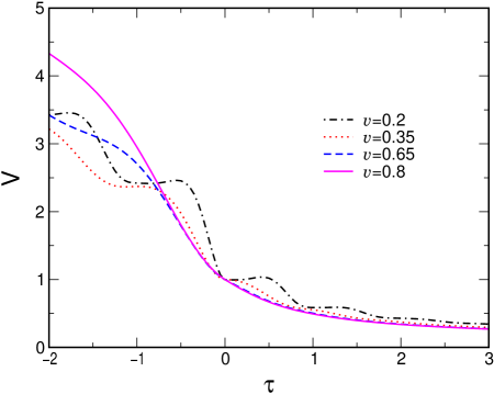
Figure 4: Elongation of vertical bonds along the path of the crack for $\eta=0.2$. Here $k=1$ and $\eta_{k}=\eta$

More interesting is the inconsistency which sets in at large velocity, and has been argued to be related to the experimentally observed microbranching. What happens here is that the elongation of the horizontal bond, given by $\vee_{hor}(\tau)=(\vee(\tau-1)-\vee(\tau))/2$ increases as a function of increasing driving. At some critical speed it reaches the value $\vee(0)$ and the bond breaks. Figure 5 shows the dependence of the critical speed on $\eta$. We note in passing that these graphs agree with what can be gotten by extrapolating a similar graph for the finite $N_{y}$ lattice, a graph that can be obtained using the methods of (Kessler and Levine, 1998). The actual location in $\tau$ at which the horizontal break occurs at the critical velocity is shown in Fig. 6.

Several details of our findings are worthy of note. First, there is always a critical speed for any dissipation, but this speed gets very close to the maximal crack speed for large $\eta$. The value of the critical speed for the dissipation-less limit is $v_{cr}\simeq.725$; this is above what has been seen in some experiments but recall that we are doing mode III on a square lattice, a far cry from mode I in an amorphous system. The is a curious break in the curve at $\eta\simeq.665$, which corresponds in Fig. 6 to the point where the break location varies most strongly with $\eta$.

It should be noted that this inconsistency does not appear related in any obvious way to the Yoffe (1951) criterion. First, the Yoffe criterion, concerning the direction of maximal stress, is calculated for the continuum elastic field, and is thus completely independent of the viscosity $\eta$ (Kessler and Levine, 1998). The onset of the inconsistency is strongly $\eta$ dependent however. Also, the Yoffe criterion is stated for Mode I cracks, and its applicability to Mode III is subject to question.

We turn now to the case of $k<1$, with weakened bonds along the crack path, again keeping $\eta_{k}=\eta$. Figures 5, 6 show our results. As is reasonable, the inconsistencies persist, but are pushed to higher speeds as $k$ decreases. It is interesting to speculate that since for finite width systems, velocities greater than the wave speed are possible, sufficiently small $k$ might enable stable steady-state fracture at supersonic velocities. Also, intersonic wave speeds are possible in the case of mode II fracture, and therefore weakened bonds on the path of the crack would in this case as well allow steady-state propagation at higher speeds (Rosakis, et al., 1999).

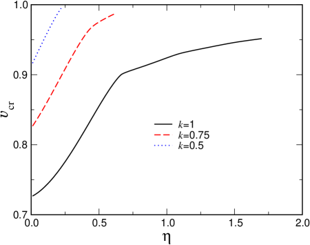
Figure 5: Dependence of the critical speed $v_{cr}$ on $\eta$ for $k=1$, $0.75$, $0.5$. Here $\eta_{k}=\eta$

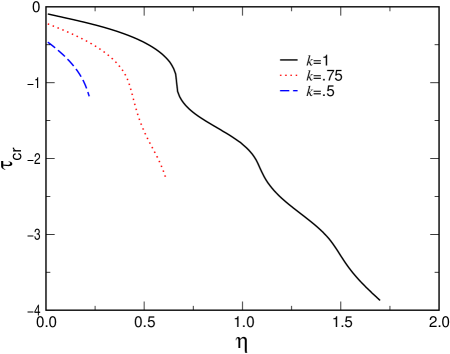
Figure 6: Dependence of the critical time $\tau_{cr}$ on $\eta$ for $k=1$, $0.75$, $0.5$. Here $\eta_{k}=\eta$.

VI Discussion

We have shown how to extend the Slepyan approach to cracks in ideally brittle infinite lattice systems to the case of having a Kelvin viscosity for each lattice spring. In addition, we have examined the onset of the additional, off-axis cracking at high velocity. We showed how dissipation delays but does not eliminate the microbranching instability, an effect impossible to see within the context of any continuum elastic treatment.

In the following work, we will present the results of similar calculations for mode I cracks on a triangular lattice. That system is much closer to those that have been studied experimentally and one can therefore hope for more direct lessons to emerge. Also, we should mention complementary studies on nonlinear lattice models which relax the assumption of ideally brittle springs and thereby allow one to view the onset of inconsistent behavior as the limiting case of more standard bifurcations (Kessler and Levine, 1999, 2000).

VII Appendix

We discuss here some of our conventions and notations regarding Fourier transformations. We use Fourier transformation in the form

$$u^{F}(q)=\int_{-\infty}^{+\infty}u(\tau)e^{iq\tau}d\tau$$

$$u(\tau)=\frac{1}{2\pi}\int_{-\infty}^{+\infty}u^{F}(q)e^{-iq\tau}dq$$ (55)

We define also $u^{+}$ and $u^{-}$ as

$$u^{+}(q) = \int_{0}^{+\infty}u(\tau)e^{iq\tau}d\tau$$ (56a)

$$u^{-}(q) = \int_{-\infty}^{0}u(\tau)e^{iq\tau}d\tau$$ (56b)

This gives

$$u(\tau)\theta(\tau) = \frac{1}{2\pi}\int_{-\infty}^{+\infty}u^{+}(q)e^{-iq\tau}dq\ ;$$ (57a)

$$u(\tau)\theta(-\tau) = \frac{1}{2\pi}\int_{-\infty}^{+\infty}u^{-}(q)e^{-iq\tau}dq\ ,$$ (57b)

which means that $u^{+}$ has poles only in the lower half plane and $u^{-}$ only in the upper half plane.

Now let us define $p=-iq$. Then

$$\int_{0}^{+\infty}u(\tau)e^{iq\tau}d\tau\stackrel{{{}_{p\rightarrow+\infty}}}{{\sim}}u(0)\int_{0}^{+\infty}e^{-p\tau}d\tau=\frac{1}{p}u(0)\ .$$ (58)

Thus

$$\lim_{-iq\rightarrow+\infty}{-iqu^{+}}=u(0)\ .$$ (59)

Similarly we can get for $p=iq$

$$\int_{-\infty}^{0}u(\tau)e^{iq\tau}d\tau\stackrel{{{}_{p\rightarrow+\infty}}}{{\sim}}u(0)\int_{-\infty}^{0}e^{p\tau}d\tau=\frac{1}{p}u(0)\ .$$ (60)

So

$$\lim_{iq\rightarrow+\infty}{iqu^{-}}=u(0)\ .$$ (61)

The Fourier transform of $\theta(-\tau)\frac{d}{d\tau}u(\tau)$ is given by

$$\int_{-\infty}^{0}\frac{du(\tau)}{d\tau}e^{iq\tau}d\tau=u(0)-iqu^{-}$$ (62)

Finally, we consider separating an arbitrary function $S(q)$ into the product of two pieces $S^{+}$ and $S^{-}$, with poles and zeroes in lower and upper half-planes respectively. These can be done using the identity,

$$\frac{1}{2\pi i}\int_{-\infty}^{+\infty}\frac{\ln S(\xi)}{\xi-q}d\xi=\frac{1}{2\pi i}\int_{-\infty}^{+\infty}\left(\frac{\ln S^{+}(\xi)}{\xi-q}+\frac{\ln S^{-}(\xi)}{\xi-q}\right)d\xi$$

$$\ =\ \ \ \ \ \left\{\begin{array}[]{ll}for\;\;Im\;q>0,&\;\;\ln S^{+}(q)\\ for\;\;Im\;q<0,&\;-\ln S^{-}(q)\end{array}\right.\ .$$ (65)

References

- Abraham, et al. (1994) Abraham, F.F., Brodbeck, D., Rafey, R.A., Rudge, W.E., 1994. Instability dynamics of fracture - a computer-simulation investigation. Phys. Rev. Lett. 73 (2), 272-275.
- Barenblatt (1959) Barenblatt, G.I., 1959. The formation of equilibrium cracks during brittle fracture: General ideas and hypothesis, axially symmetric cracks. Appl. Math. and Mech. 23, 622-636 (1959).
- Fineberg, et al. (1991) Fineberg, J., Gross, S.P., Marder, M., Swinney, H.L., 1991. Instability in dynamic fracture. Phys. Rev. Lett. 67, (4) 457-460.
- Fineberg, et al. (1992) Fineberg, J., Gross, S.P., Marder, M., Swinney, H.L., 1992. Instability in the propagation of fast cracks. Phys. Rev. B45, (10) 5146-5154.
- Fineberg and Marder (1999) Fineberg, J., Marder, M., 1999. Instability in dynamic fracture. Phys. Repts. 313, (1-2) 1-108.
- Gumbsch, et al. (1997) Gumbsch, P., Zhou, S.J., Holian, B.L., 1997. Molecular dynamics investigation of dynamic crack stability. Phys. Rev. B55 (6), 3445-3455.
- Holland and Marder (1997) Holland, D., Marder, M., 1997. Ideal brittle fracture of silicon studied with molecular dynamics. Phys. Rev. Lett. 80, (4) 746-749.
- Holland and Marder (1998) Holland, D., Marder, M., 1998. Erratum: Ideal brittle fracture of silicon studied with molecular dynamics. Phys. Rev. Lett. 81, (18) 4029.
- Kessler (2000) Kessler, D.A., 2000. Steady-state cracks in viscoelastic lattice models II. Phys. Rev. E, to appear.
- Kessler and Levine (1998) Kessler, D.A., Levine, H., 1998. Steady-state cracks in viscoelastic lattice models. Phys. Rev. E59 (5), 5154-5164.
- Kessler and Levine (1999) Kessler, D.A., Levine, H., 1999. Arrested cracks in nonlinear lattice models of brittle fracture. Phys. Rev. E60 (6) 7569-7571.
- Kessler and Levine (2000) Kessler, D.A., Levine, H., 2000. Stability of Cracks in Nonlinear Viscoelastic Lattice Models. In preparation.
- Kulamekhtova (1984) Kulamekhtova, Sh.A., Saraikin, V.A., Slepyan, L.I., 1984. Plane problem of a crack in a lattice. Izv. AN SSSR. Mekhanika Tverdogo Tela, 19, (3) 112-118 [Mech. Solids 19, (3) 102-108].
- Langer (1992) Langer, J.S., 1992. Models of crack propagation. Phys. Rev. E46 (6), 3123-3131.
- Langer and Lobkovsky (1998) Langer, J.S., Lobkovsky, A.E., 1998. Critical examination of cohesive-zone models in the theory of dynamic fracture. J. Mech. Phys. Solids 46 (9), 1521-1556.
- Marder and Gross (1995) Marder, M., Gross, S.P., 1995. Origin of crack tip instabilities. J. Mech. Phys. Solids 43 (1), 1-48.
- Marder and Liu (1993) Marder, M., Liu, X., 1993. Instability in lattice fracture. Phys. Rev. Lett. 71 (15), 2417-2420.
- Omeltchenko, et al. (1997) Omeltchenko, A., Yu, J., Kalia, R.K., Vashishta, P., 1997. Crack front propagation and fracture in a graphite sheet: a molecular-dynamics study on parallel computers. Phys. Rev. Lett. , 78 (11), 2148-2151.
- Pechenik, et al. (2000) Pechenik, L., Levine, H., Kessler, D.A., 2000. Steady-state mode I cracks in a viscoelastic triangular lattice. Submitted for publication
- Pla, et al. (1998) Pla, O., Guinea, F., Louis, E.,Ghasias, S.V., Sander, L.M., 1998. Viscous effects in brittle fracture. Phys. Rev. B57 (22), R13981-R13984.
- Rosakis, et al. (1999) Rosakis, A.J., Samudrala, O., Coker, D., 1999. Cracks faster than the shear wave speed. Science 284 (5418), 1337-40.
- Sander and Ghasias (1999) Sander, L.M., Ghasias, S.V., 1999. Thermal noise and the branching threshold in brittle fracture. Phys. Rev. Lett. 83, (10) 1994-1997.
- Sharon, et al. (1995) Sharon, E., Gross, S.P. and Fineberg, J., 1996. Local crack branching as a mechanism for instability in dynamic fracture. Phys. Rev. Lett. 74 (25), 5096-5099.
- Sharon, et al. (1996) Sharon, E., Gross, S.P. and Fineberg, J., 1996. Energy dissipation in dynamic fracture. Phys. Rev. Lett. 76 (12), 2117-2120.
- Slepyan (1981) Slepyan, L.I., 1981. Dynamics of a crack in a lattice. Doklady Akademii Nauk SSSR 258 (1-3) 561-564. [Sov. Phys. Dokl. 26 (5), 538-540].
- Slepyan (1982) Slepyan, L.I., 1982.The relation between the solutions of mixed dynamical problems for a continuous elastic medium and a lattice. Doklady Akademii Nauk SSSR, 266 (1-3) 581-584. [Sov. Phys. Dokl. 27 (9), 771-772.
- Yoffe (1951) Yoffe, E.Y., 1951. Philos. Mag. 42, 739-750.
- Zhou, et al. (1997) Zhou, S.J., Beazley, D.M., Lomdahl, P.S., Holian, B.L., 1997. Large-scale molecular dynamics simulations of three-dimensional ductile failure. Phys. Rev. Lett. 78 (3), (479-482).