[

Boundary-induced phase transitions in traffic flow

Abstract

Boundary-induced phase transitions are one of the surprising phenomena appearing in nonequilibrium systems. These transitions have been found in driven systems, especially the asymmetric simple exclusion process. However, so far no direct observations of this phenomenon in real systems exists. Here we present evidence for the appearance of such a nonequilibrium phase transition in traffic flow occurring on highways in the vicinity of on- and off-ramps. Measurements on a German motorway close to Cologne show a first-order nonequilibrium phase transition between a free-flow phase and a congested phase. It is induced by the interplay of density waves (caused by an on-ramp) and a shock wave moving on the motorway. The full phase diagram, including the effect of off-ramps, is explored using computer simulations and suggests means to optimize the capacity of a traffic network.

]

One-dimensional physical systems with short-ranged interactions in thermal equilibrium do not exhibit phase transitions. This is no longer true if the action of external forces sets up a steady mass transport and drives the system out of equilibrium. Then boundary conditions, usually insignificant for an equilibrium system, can induce nonequilibrium phase transitions. Moreover, such phase transitions may occur in a rather wide class of driven complex systems, including biological and sociological mechanisms involving many interacting agents. In spite of the importance of this phenomenon and a number of theoretical studies [1, 2, 3, 4], it has never been observed directly. So far only indirect experimental evidence for a boundary-induced phase transition exists in older studies of the kinetics of biopolymerization on nucleic acid templates [5, 6].

In the present work we report the first direct observation of a boundary-induced phase transition in traffic flow. Analysis of traffic data sets taken on a motorway near Cologne exhibits transitions from free-flow traffic to congested traffic, caused by a boundary effect, viz. the presence of an on-ramp. These transitions are characterized by a discontinuous reduction of the average speed [7].

Vehicular traffic on a motorway is controlled by a mixture of bulk and boundary effects caused by on- and off-ramps, varying number of lanes, speed limits, leaving aside temporary effects of changing weather conditions and other non-permanent factors. The fundamental characteristic of the bulk motion is the stationary flow-density diagram, i.e. the fundamental diagram, which incorporates the collective effects of individual drivers behavior such as trying to maintain an optimal high speed while keeping safety precautions. The qualitative shape of the flow-density diagram $j(\rho)$ is largely independent of the precise details of the road and hence amenable to numerical analysis using either stochastic lattice gas models or partial differential equations [8, 9].

A by now well-established lattice gas model for traffic flow, the cellular automaton model by Nagel and Schreckenberg [10], reproduces empirical traffic data [11] rather well. Fig. 1 shows simulation data for the fundamental diagram obtained from the Nagel-Schreckenberg (NaSch) model. This has to be compared to measurements of the flow $j$ taken with the help of detectors on the motorway A1 near Cologne which show a maximum of about 2000 vehicles/hour at a density of about $\rho^{\ast}=20$ vehicles per lane and km [7]. At densities below $\rho^{\ast}$ one observes free flow, while for larger densities one observes congested traffic.

FIG. 1.: Fundamental diagram (flow-density-relation) as modeled by the NaSch model with $v_{max}=4,\ p=0.25$, time step =$1.0$ sec, lattice spacing =$7.5$ m. The system has 3200 sites, and the flux is averaged over $10^{6}$ lattice updates. The broken and full lines indicate the slope which defines the collective velocity of spontaneous local traffic jams and the shock velocity, respectively.

In addition to the density dependence of the flow two important characteristics are derived directly from the fundamental diagram: the shock velocity of a ‘domain wall’ [12] between two stationary regions of densities $\rho^{-},\rho^{+}$

$$v_{shock}=\frac{j(\rho^{+})-j(\rho^{-})}{\rho^{+}-\rho^{-}},$$ (1)

obtained from mass conservation, and the collective velocity

$$v_{c}=\frac{\partial j(\rho)}{\partial\rho}$$ (2)

which is the velocity of the center of mass of a local perturbation in a homogeneous, stationary background of density $\rho$. Both velocities are readily observed in real traffic. The collective velocity $v_{c}$ describes the upstream movement of a local, compact jam. In the density range $25\dots 130$ cars/km $v_{c}$ ranges from approximately $-10$ km/hour to $-20$ km/hour (Fig. 1) which has to be compared with the empirically observed value $v\approx-15$ km/hour [10, 13]. The shock velocity is the velocity of the upstream front of an extended, stable traffic jam. The formation of a stable shock is usually a boundary-driven process, caused by a ‘bottleneck’ on a road. Bottlenecks on a highway arise from a reduction in the number of lanes and from on-ramps where additional cars enter a road [14, 15].

The experimental data considered here (see Fig. 2 for the relevant part of the highway) show boundary effects caused by the presence of an on-ramp. Far upstream from the on-ramp, free flow of vehicles with density $\rho^{-}$ and flow $j^{-}\equiv j(\rho^{-})$ is maintained. Just before the on-ramp the vehicle density is $\rho^{+}$ with corresponding flow $j^{+}\equiv j(\rho^{+})$. Note that no experimental data are available for $\rho^{-}$, $j^{-}$ and $\rho^{+}$, $j^{+}$ as well as the activity of the ramp. The only data come from a detector located upstream from the on-ramp [16] which measures a traffic density $\hat{\rho}$ and the corresponding flow $\hat{\jmath}$.

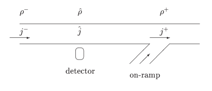
FIG. 2.: Schematic road design of a highway with an on-ramp where cars enter the road. The arrows indicate the direction of the flow. The detector measures the local bulk density $\hat{\rho}$ and bulk flow $\hat{\jmath}$.

Next the effects of the on-ramp are considered. Cars entering the motorway cause the mainstream of vehicles to slow down locally. Therefore, the vehicle density just before the on-ramp increases to $\rho^{+}>\rho^{-}$. Then a shock, formed at the on-ramp, will propagate with mean velocity $v_{shock}$ (see (1)). Depending on the sign of $v_{shock}$, two scenarios are possible:
1) $v_{shock}>0$ (i.e. $j^{+}>j^{-}$): In this case the shock propagates (on average) downstream towards the on-ramp. Only by fluctuations a brief upstream motion is possible. Therefore the detector will measure a traffic density $\hat{\rho}=\rho^{-}$ and flow $\hat{\jmath}=j^{-}$.
2) $v_{shock}<0$ (i.e. $j^{+}<j^{-}$): The shock wave starts propagating with the mean velocity $v_{shock}$ upstream, thus expanding the congested traffic region with density $\rho^{+}$. The detector will now measure $\hat{\rho}=\rho^{+}$ and flow $\hat{\jmath}=j^{+}$.

Let us now discuss the transition between these two scenarios. Suppose one starts with a situation where $j^{+}>j^{-}$ is realized. If now the far-upstream-density $\rho^{-}$ increases it will reach a critical point $\rho_{crit}<\rho^{\ast}$ above which $j^{-}>j^{+}$, i.e., the free flow upstream $j^{-}$ prevails over the flow $j^{+}$ which the ‘bottleneck’, i.e. the on-ramp, is able to support. At this point shock wave velocity $v_{shock}$ will change sign (see (1)) and the shock starts traveling upstream. As a result, the stationary bulk density $\hat{\rho}$ measured by the detector upstream from the on-ramp will change discontinuously from the critical value $\rho_{crit}$ to $\rho^{+}$. This marks a nonequilibrium phase transition of first order with respect to order parameter $\hat{\rho}$. The discontinuous change of $\hat{\rho}$ leads also an abrupt reduction of the local velocity. Notice that the flow $\hat{\jmath}=j^{+}$ through the on-ramp (then also measured by the detector) will stay independent of the free flow upstream from the congested region $j^{-}$ as long as the condition $j^{-}>j^{+}$ holds.

Empirically this phenomenon can be seen in the traffic data taken from measurements at the detector D1 on the motorway A1 close to Cologne [7]. Fig. 3 shows a typical time series of the one-minute velocity averages. One can clearly see the sharp drop of the velocity at about 8 a.m.

FIG. 3.: Time series of the velocity. Each data point represents an one-minute average of the speed. Shown are empirical data (from [7]) in comparison with the results of computer simulations of a simplified model (see text).

Also the measurements of the flow versus local density, i.e. the fundamental diagram (Fig. 4), support our interpretation. Two branches can be distinguished. The increasing part corresponds to an almost linear rise of the flow with density in the free-flow regime [13]. In accordance with our considerations this part of the flow diagram is not affected by the presence of the on-ramp at all and one measures $\hat{\jmath}=j^{-}$ which is the actual upstream flow. The second branch are measurements taken during congested traffic hours, the transition period being omitted for better statistics. The transition from free flow to congested traffic is characterized by a discontinuous reduction of the local velocity. However, as predicted above the flow does not change significantly in the congested regime. In contrast, in local measurements large density fluctuations can be observed. Therefore in this regime the density does not take the constant value $\rho^{+}$ as suggested by the argument given above, but varies from 20 veh/km/lane to 80 veh/km/lane (see Fig. 4).

One should stress here that congested traffic data are usually not easy to interpret, because the traffic conditions (mean inflow and outflow of cars on the on- and off-ramps, and so the bulk mean flow) are changing in time. According to our arguments, in a congested regime the detector measures $j^{+}$, solely due to the on-ramp activity. Therefore, $j^{+}(t)=j(\rho^{+}(t))<j^{-}(t)$ must be satisfied. During times of very dense traffic one expects always cars ready to enter the motorway at the on-ramp, thus guaranteeing a sufficient and approximately constant on-ramp activity. The measured flow is constant over long periods of time which is in agreement with the notion that the transition is due a stable traffic jam. Spontaneously emerging and decaying jams would lead to the observation of a non-constant flow.

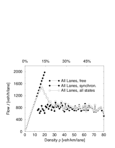
FIG. 4.: Measurements of the flow versus local density before an on-ramp on the motorway A1 close to Cologne. The detector is located at a distance 1 km upstream from on-ramp. Data are collected over a period of 12 days.

The use of our approach is not limited to a qualitative explanation of the traffic data. Beyond that it can also be used to calculate the phase diagrams of systems with open boundary conditions for a large class of traffic models. We modeled a section of a road with on-ramp on the left and off-ramp (on-ramp) on the right using the NaSch cellular automaton [10]. We modify the basic model by using open boundary conditions with injection of cars at the left boundary (corresponding to in-flow into the road segment) and removal of cars at the right boundary (corresponding to outflow). Therefore it can also be regarded as a generalization of the asymmetric simple exclusion process [17] to particles with higher velocity.

During the simulations local measurements of the velocity have been performed analogous to the experimental setup. For comparison the results of the computer simulations have been included in Fig. 3. Note that even the quantitive agreement with the empirical data is very good. This has been achieved by using a finer discretization of the model, i.e. the length of the cell is considered as $l=2.5m$. The results were obtained for $L=960$, $p=0.25$ and $v_{max}=13$. We kept the input probability $\alpha=0.65$ constant. Then the free-flow part is obtained using $\beta=1.$ and the congested part using $\beta=0.55$. The transition was observed at ten minutes after we reduced the output probability. The “detector” was located at the link from site $480$ to $481$.

Fig. 5 shows the full phase diagram of the NaSch model with open boundary conditions. It describes the stationary bulk density $\hat{\rho}$ as a function of the far-upstream in-flow boundary density $\rho^{-}$ and the effective right boundary density $\rho^{+}$. For the case of an on-ramp (or shrinking road width etc.) at the right boundary corresponds to the situation discussed above. Here, the density is increased locally to $\rho^{+}>\rho^{-}$. In agreement with the empirical observation we find a line of first order transitions from a free flow (FF) phase with bulk density $\hat{\rho}=\rho^{-}$ to a congested (CT) phase with $\hat{\rho}=\rho^{+}$. On this line $v_{shock}$ changes sign.

FIG. 5.: Phase diagram of the NaSch model with open boundaries for $p=0.25,v_{max}=4$. Cars enter the road from a reservoir of density $\overline{\rho^{-}}$, inducing the upstream-density $\rho^{-}$ discussed in the text. At the right boundary cars leave the road into a reservoir of density $\overline{\rho^{+}}$, leading to the on-ramp density $\rho^{+}$. The solid (dashed) curve denotes the theoretical prediction for the first (second) order transitions lines obtained from the numerically determined flow-density relation. The points represent phase transition points for the simulated system of size 3200. The phases are: free flow (FF), congested traffic (CT), maximal flow (MF) phase.

The case of an off-ramp (or expansion of road space etc.) leads to a local decrease $\rho^{+}<\rho^{-}$ of the density. Here the collective velocity $v_{c}$ (2) plays a prominent role. As long as $v_{c}$ is positive (i.e. in the free-flow regime $\rho^{-}<\rho^{\ast}$, see Fig. 1), perturbations caused by a small increase of the upstream boundary density $\rho^{-}$ gradually spread into the bulk, rendering $\hat{\rho}=\rho^{-}$ (FF regime). At $\rho^{-}=\rho^{\ast}$, $v_{c}$ changes sign [18] and an overfeeding effect occurs: a perturbation from the upstream boundary does not spread into the bulk [2, 4] and therefore further increase of the upstream boundary density does not increase the bulk density. The system enters the maximal flow (MF) phase with constant bulk density $\hat{\rho}=\rho^{\ast}$ and flow $j(\rho^{\ast})=j_{max}$. The transition to the MF phase is of second order, because $\hat{\rho}$ changes continuously across the phase transition point.

The existence of a maximal flow phase was not emphasized in the context of traffic flow up to now. At the same time, it is the most desirable phase, carrying the maximal possible throughput of vehicles $j_{max}$. For practical purposes our observations may directly be used in order to operate a highway in the optimal regime. E.g. the flow near a lane reduction could be increased significantly if the traffic state at the entry would allow to attain the maximal possible flow of the bottleneck. This could be achieved by controlling the density far upstream, e.g. by closing temporally an on-ramp, such that the cars still enter the bottleneck with high velocity.

We stress that the stationary phase diagram Fig. 5 is generic in the sense that it is determined solely by the macroscopic flow-density relation. The number of lanes of the road, the distribution of individual optimal velocities, speed limits, and other details enter only in so far as they determine the exact values characterizing the flow-density relation for that particular road. We also note that throughout the paper we assumed the external conditions to vary slowly, so that the system has enough time to readjust to its new stationary state. Experimenting with different cellular traffic models in a real time scale shows that the typical time to reach a stationary state in a road segment of about 1.2 km is of the order of 3-5 min, which is reasonably small. Close to phase transitions lines, however, where the shock velocity vanishes, this time diverges and intrinsically non-stationary dynamic phenomena [19, 20] take the lead.

In conclusion, we have shown that traffic data collected on German motorways provide evidence for a boundary-induced nonequilibrium phase transition of first order from the free flowing to the congested phase. The features of this phenomenon are readily understood in terms of the flow-density diagram. The dynamical mechanism leading to this transition is an interplay of shocks and local fluctuations caused by an on-ramp. Full investigation of a cellular automaton model for traffic flow reproduces this phase transition, but also exhibits a richer phase diagram with an interesting maximal flow phase. These results are not only important from the point of view of nonequilibrium physics, but also suggest new mechanisms of traffic control.

Acknowledgments: We thank Lutz Neubert for useful discussions and help in producing Figs. 3 and 4. L. S. acknowledges support from the Deutsche Forschungsgemeinschaft under Grant No. SA864/1-1.

REFERENCES

- [1] Krug, J., Phys. Rev. Lett. 67, 1882 (1991).
- [2] Schütz, G. and Domany, E., J. Stat. Phys. 72, 277 (1993).
- [3] Oerding, K., and Janssen, H.K., Phys. Rev. E 58, 1446 (1998).
- [4] Kolomeisky, A.B., Schütz, G.M., Kolomeisky, E.B. and Straley, J.P., J.Phys. A 31, 6911 (1998).
- [5] MacDonald, J.T. and Gibbs J.H., Biopolymers 7, 707 (1969).
- [6] Schütz, G.M., Int. J. Mod. Phys. B 11, 197 (1997).
- [7] Neubert, L., Santen, L., Schadschneider, A. and Schreckenberg, M., Phys. Rev. E 60, 6480 (1999).
- [8] Chowdhury, D., Santen, L., and Schadschneider, A., Curr. Sci. 77, 411 (1999) and Physics Reports (in press).
- [9] Helbing, D., Verkehrsdynamik: Neue Physikalische Modellierungskonzepte (in German) (Springer, Berlin, 1997).
- [10] Nagel, K. and Schreckenberg, M., J. Phys. I France 2, 2221 (1992).
- [11] Hall, F.L., Allen, B.L. and Gunter, M.A., Transp. Res. A 20, 197 (1986).
- [12] In nonequilibrium systems a domain wall is an object connecting two possible stationary states.
- [13] Kerner, B.S. and Rehborn, H., Phys. Rev. E 53, R4275 (1997). For the situation studied in this paper the front velocity of the jam can be identified with its center-of-mass velocity.
- [14] Daganzo, C.F., Cassidy, M.J. and Bertini R.L., Transp. Res. A 33, 365 (1999).
- [15] G. Diedrich, L. Santen, A. Schadschneider and J. Zittartz, Int. J. Mod. Phys. C (in press)
- [16] The distance between the detector and the on-ramp should be large enough, so that the on-ramp fluctuations are not measured directly. In our case, the detector is located approximately 1 km upstream from on-ramp.
- [17] see e.g. G.M. Schütz, Exactly solvable models for many-body systems far from equilibrium, to appear in Phase Transitions and Critical Phenomena, C. Domb und J. Lebowitz (eds.), (Academic Press, London, 2000); T.M. Liggett, Stochastic Interacting Systems: Contact, Voter and Exclusion Processes (Springer, Berlin, 1999); and the contributions by B. Derrida, M.R Evans and S.A. Janowsky, J.L. Lebowitz in V. Privman (ed.), Nonequilibrium Statistical Mechanics in One Dimension, (Cambridge University Press, Cambridge, 1997).
- [18] In this case the upstream entrance to the road itself acts as a ‘dynamical’ bottleneck with maximal capacity .
- [19] Kerner, B.S. and Rehborn, H., Phys. Rev. Lett. 79, 4030 (1997).
- [20] Lee, H.Y., Lee, H.-W. and Kim, D., Phys. Rev. Lett. 81, 1130 (1998).