Canonical solution of a system of long-range interacting rotators on a lattice

Alessandro Campa¹, Andrea Giansanti^2,§ and Daniele Moroni²

¹Physics Laboratory, Istituto Superiore di Sanità and INFN Sezione di Roma1, Gruppo Collegato Sanità

Viale Regina Elena 299, 00161 Roma, Italy

²Physics Department, Università di Roma “La Sapienza” and INFM Unità di Roma1,

Piazzale Aldo Moro 2, 00185 Roma, Italy

(13 April 2000, accepted for publication in Physical Review E)

Abstract

The canonical partition function of a system of rotators (classical X-Y spins) on a lattice, coupled by terms decaying as the inverse of their distance to the power $\alpha$, is analytically computed. It is also shown how to compute a rescaling function that allows to reduce the model, for any $d$-dimensional lattice and for any $\alpha<d$, to the mean field ($\alpha=0$) model. PACS: 05.20.-y, 05.70.Ce, 05.10.-a

^§ Author to whom correspondence should be addressed; electronic address: Andrea.Giansanti@roma1.infn.it

1 Introduction

Let us consider the following classical hamiltonian model of a system of rotators:

$$H=\frac{1}{2}\sum_{i=1}^{N}L_{i}^{2}\,+\,\frac{1}{2}\sum_{i,j=1}^{N}\left[1-\cos(\theta_{i}-\theta_{j})\right]=K+V\,.$$ (1)

The potential energy $V$ is not thermodynamically stable and the ensemble averaged energy density $U=\langle\frac{H}{N}\rangle$ diverges in the thermodynamic limit (TL) [1]. If the potential energy term is divided by $N$, then the energy density becomes intensive and it is bounded as $N$ goes to infinity.

Indeed, dynamics and thermodynamics of the $1/N$ rescaled model has been extensively investigated [2]; in particular, Ruffo and Antoni, who called it the hamiltonian mean field X-Y model (HMF), solved it in the canonical ensemble, and compared the theoretical caloric ($T\,vs\,U$) and magnetization ($M\,vs\,U$) curves with those obtained from a microcanonical simulation [3].

Here we consider a generalization of model (1):

$$H=\frac{1}{2}\sum_{i=1}^{N}L_{i}^{2}\,+\,\frac{1}{2}\sum_{i\neq j}^{N}\frac{1-\cos(\theta_{i}-\theta_{j})}{r_{ij}^{\alpha}}\,.$$ (2)

The rotators are placed at the sites of a lattice and the interaction between rotators $i$ and $j$ decays as the inverse of their distance to the power $\alpha$.

A onedimensional version of model (2) has been studied by Anteneodo and Tsallis [4], who have numerically measured the largest Lyapounov exponent, as a function of $N$ and $\alpha$. Through a rescaling factor $N^{*}=\frac{N^{1-\alpha}-1}{1-\alpha}$ Anteneodo and Tsallis showed that their results coincide with those previously obtained for the HMF ($\alpha=0$) model; this rescaling could then give a well defined TL to model (2).

In a recent paper Tamarit and Anteneodo, using a rescaling factor $\tilde{N}=2^{\alpha}\frac{N^{1-\alpha}-1}{1-\alpha}$, have shown that the caloric and magnetization curves of model (2) in one dimension collapse onto the curves of the HMF model [5]. This universality emerges plotting $T/\tilde{N}$ as a function of $H/N\tilde{N}$ and $M$ as a function of $H/N\tilde{N}$, from molecular dynamics simulation of model (2) for different $N$ and $\alpha$ values. These authors conjecture that the results they obtained in the onedimensional case might be general, valid in any dimension $d$ and for $\alpha<d$, as suggested also in [5].

2 Partition function

In this work, inspired by [3] and [5], we analytically compute the partition function of an $\tilde{N}$-rescaled model (2) for any $d$ and $\alpha<d$. In formula (21) we give the right expression of the rescaling function $\tilde{N}$, to obtain universal state curves for all lattice models with long range ($\alpha<d$) interactions.

Let us now rewrite the rescaled version of Hamiltonian (2):

$$H = \frac{1}{2}\sum_{i=1}^{N}L_{i}^{2}\,+\,\frac{1}{2\tilde{N}}\sum_{i,j=1}^{N}\frac{1-\cos(\theta_{i}-\theta_{j})}{r_{ij}^{\alpha}}$$ (3)

$$-h_{x}\sum_{i=1}^{N}m_{ix}-h_{y}\sum_{i=1}^{N}m_{iy}\,,$$

where we have introduced an external magnetic field $\mathbf{h}=(h_{x},h_{y})$ of modulus $h$, that makes possible to compute the magnetization. The indexes $i,j$ label the sites of a $d$-dimensional generic lattice; $r_{ij}$ is the distance between them, with periodic boundary conditions and nearest image convention (the definition of $r_{ii}$ will be given shortly); $\alpha\geq 0$. At each site a classical rotator (X-Y spin) of unit momentum of inertia is represented by conjugate canonical coordinates $(L_{i},\theta_{i})$, where the $L_{i}$’s are angular momenta, and the $\theta_{i}$’s $\in[0,2\pi)$ are the angles of rotation on a family of parallel planes, each one defined at each lattice point; $x$ and $y$ refer to the components of boldface twodimensional vectors defined over these planes. To each lattice site a spin vector

$$\mathbf{m}_{i}=(m_{ix},m_{iy})=(\cos\theta_{i},\sin\theta_{i})$$ (4)

is associated, and the total magnetization is given by:

$$\mathbf{M}=(M_{x},M_{y})=\frac{1}{N}\sum_{i=1}^{N}\mathbf{m}_{i}\,.$$ (5)

Note in (3) the rescaling factor $\tilde{N}$ in front of the potential energy term, now written as a free double sum over both indexes. $\tilde{N}$ should be regarded as an unknown function of $N,\alpha,d$ and the geometry of the lattice, with the fundamental property of making

$$\frac{1}{\tilde{N}}\sum_{j,j\neq i}\frac{1}{r_{ij}^{\alpha}}$$ (6)

an intensive quantity; this guarantees the thermodynamic stability of the potential. We also note that the sum in (6) is independent of the origin $i$ because of periodic conditions. To reproduce the usual HMF it is also necessary that $\tilde{N}(N,\alpha=0,d)=N$. The constraint $i\neq j$ over the double sum is removed defining $r_{ii}^{\alpha}=1/b$, a finite number. Since the numerator $1-\cos(\theta_{i}-\theta_{j})$ is zero for $i=j$ the choice of $b$ is free. The removal of the constraint allows to introduce the distance matrix $R^{\prime}_{ij}=\frac{1}{r_{ij}^{\alpha}}$; the diagonalization of such matrix is the key point to obtain, in the computation of the partition function, known integrals in the variables $\theta_{i}$.

As usual the partition function factorizes in a kinetic part $Z_{K}=\left(\frac{2\pi}{\beta}\right)^{\frac{N}{2}}$, where $\beta=1/k_{B}T$, and a potential part $Z_{V}$. After defining $R_{ij}=\frac{\beta}{2\tilde{N}}R^{\prime}_{ij}$, $\mathbf{B}=\beta\mathbf{h}$, $C=\exp\left(-\frac{\beta}{2\tilde{N}}\sum_{ij}\frac{1}{r_{ij}^{\alpha}}\right)$, the potential part can be written as:

$$Z_{V}=C\int_{-\pi}^{\pi}d^{N}\theta\,\exp\left[\sum_{i,j,\mu}m_{i\mu}R_{ij}m_{j\mu}+\sum_{i}B_{\mu}m_{i\mu}\right],$$ (7)

where $\mu=x,y$. Diagonalizing the symmetric matrix $R=(R_{ij})$ with the unitary matrix $U$ such that $R=U^{T}DU$, $D=(R_{i}\delta_{ij})$, where $R_{i}$ are the eigenvalues of $R$, we can write the first part of the exponent in (7) as:

$$\sum_{ij}\left(m_{ix}R_{ij}m_{jx}+m_{iy}R_{ij}m_{jy}\right)=\sum_{i}\left(n_{ix}^{2}R_{i}+n_{iy}^{2}R_{i}\right),$$ (8)

where $n_{i\mu}=\sum_{j}U_{ij}m_{j\mu}$. In order to apply the gaussian transformation:

$$e^{aS^{2}}=\frac{1}{\sqrt{4\pi a}}\int_{-\infty}^{+\infty}dze^{-\frac{z^{2}}{4a}+Sz}\,\,\,\,a>0$$ (9)

to each term of the sum in the right hand side of (8), each $R_{i}$ must be positive. The spectrum can be explicitly computed using a $d$-dimensional Fourier transform of matrix $R$, the eigenvalues being labelled by vectors of the reciprocal lattice. These eigenvalues are trivially related to those of matrix $R^{\prime}$. A study of the spectrum of $R^{\prime}$ in the limit $N\rightarrow\infty$ and for $b=0$ shows that: when $\alpha>d$ each element of the spectrum converges to a finite quantity, the least eigenvalues being negative and of order one in modulus; when $\alpha<d$ a part of the spectrum converges to a finite quantity, another part diverges to $+\infty$, at most as $\tilde{N}$. However this last part consists of a fraction of the total number of eigenvalues which goes to zero in the limit $N\rightarrow\infty$. The least eigenvalue is still negative and of order one in modulus. Then part of the spectrum is negative, but it is easily seen that it is shifted by $b$. Thus calling $p$ the least eigenvalues of $R^{\prime}$ for $b=0$ and choosing

$$b=-p+\epsilon\quad\epsilon>0\quad,$$ (10)

we have that with this $b$ the whole spectrum of $R^{\prime}$ (and therefore that of $R$) becomes positive. Then for each $i=1,\cdots,N$, $\mu=x,y$ we can apply (9) with the correspondence $a\rightarrow R_{i}$, $S\rightarrow n_{i\mu}$, $z\rightarrow z_{i\mu}$. Performing the integrals over variables $\theta_{i}$ and using the transformation $z_{i\mu}=2\sum_{j}(UR)_{ij}\Psi_{j\mu}$ with Jacobian $2^{N}\det R$, we can rewrite the partition function as:

$$Z = CZ_{K}\frac{\det R}{\pi^{N}}\int_{-\infty}^{+\infty}d^{N}\Psi_{x}d^{N}\Psi_{y}$$

$$e^{N\left[-\sum_{ij\mu}\Psi_{i\mu}\frac{R_{ij}}{N}\Psi_{j\mu}+\frac{1}{N}\sum_{l}\ln\left(2\pi I_{0}\left(|2\sum_{j}R_{lj}\mathbf{\Psi}_{j}+\mathbf{B}|\right)\right)\right]}$$

where $I_{0}$ is the zeroth order modified Bessel function. The isolation of the $N$ factor in the exponential prepares the object for the use of the saddle point method. The quantity in square brackets is intensive. Double sums in the first two terms are compensated by $R/N=(\beta/2N\tilde{N})R^{\prime}$ and the last sum has $1/N$ in front of it. The argument of $I_{0}$ is also intensive because involves a term of the form $\sum_{j}R_{lj}=(\beta/2\tilde{N})\sum_{j}R^{\prime}_{lj}$. If we call $f(w)$ the function in square brackets, where $w=(\Psi_{1x},\cdots,\Psi_{Nx},\Psi_{1y},\cdots,\Psi_{Ny})$, then the application of the method requires the following three conditions: $f(w)$ admits a stationary point $w_{0}$; $w_{0}$ is a simple stationary point, i.e., $\det Hef|_{0}\neq 0$, where $Hef|_{0}$ is the hessian matrix of $f$ in $w_{0}$; the path of integration can be deformed (generally going into ${\cal C}^{2N}$) into a path that passes through $w_{0}$ following the steepest descent of $f(w)$ and such that $f(w)<f(w_{0})$ throughout the all path. If the point $w_{0}$ is a maximum no deformation is necessary and the method is also called the Laplace method. Since, as we show below, $w_{0}$ is indeed a real-valued maximum, we readily obtain for the free energy per particle $F$:

$$-\beta F = \lim_{N\rightarrow\infty}\frac{\ln Z}{N}=\lim_{N\rightarrow\infty}\{\frac{1}{2}\ln\left(\frac{2\pi}{\beta}\right)-\frac{\beta}{2\tilde{N}}\sum_{j}\frac{1}{r_{ij}^{\alpha}}$$ (12)

$$+\max_{w}[f(w)]+\frac{1}{N}\ln\frac{\det R}{\sqrt{\det\left(-\frac{N}{2}Hef|_{0}\right)}}\}\,.$$

The stationary point $w_{0}$ is given by the vector $(\Psi_{x},\cdots,\Psi_{x},\Psi_{y},\cdots,\Psi_{y})$, homogeneous on the lattice sites. Defining $\mathbf{\Psi}=(\Psi_{x},\Psi_{y})$, its direction is that of $\mathbf{B}$, and its modulus $\Psi$ is given by the solution of:

$$\Psi=\frac{I_{1}}{I_{0}}\left(\beta\left[A\Psi+h\right]\right)\,,$$ (13)

with

$$A=\frac{1}{\tilde{N}}\sum_{j}R^{\prime}_{ij}=\frac{1}{\tilde{N}}\left[b+\sum_{j\neq i}\frac{1}{r_{ij}^{\alpha}}\right]\,,$$ (14)

and where $I_{1}$ is the first order modified Bessel function. In (14) $A$ does not depend on $i$ because of the periodic boundary conditions. We note that when $h=0$ we have infinitely many degenerate solutions, since only the modulus $\Psi$ is determined. Evaluation of the elements of the hessian matrix at the stationary point gives:

$$\left.-\frac{N}{2}\frac{\partial^{2}f}{\partial\Psi_{i\mu}\partial\Psi_{j\nu}}\right|_{0}=R_{ij}\delta_{\mu\nu}-(R^{2})_{ij}g_{\mu\nu}(w_{0})$$ (15)

where we do not give the explicit expression of $g_{\mu\nu}(w_{0})$. As we will see shortly, the eigenvalues analysis of the hessian matrix (15) shows that the stationary point $w_{0}$ is a maximum. Then, Laplace method applies and Eq. (12) is valid. However, only in the long range case ($\alpha<d$) the last term in the rightmost side of (12) is zero; when $\alpha>d$ its expression does not appear to be manageable. We will comment on this point later. Restricting then to $\alpha<d$, and computing the derivative of (12) with respect to the magnetic field we find that the magnetization $M=\langle|\mathbf{M}|\rangle$ is given by the solution $\Psi$ of (13). Then the internal energy $U$ is given by:

$$U=\frac{\partial(\beta F)}{\partial\beta}=\frac{1}{2\beta}+\frac{A}{2}(1-M^{2})-hM\,.$$ (16)

Equations (13) and (16) are the same as those of HMF, as soon as a proper $\tilde{N}$ rescaling gives

$$A=\frac{1}{\tilde{N}}\sum_{j}R^{\prime}_{ij}=\frac{1}{\tilde{N}}\left[b+\sum_{j\neq i}\frac{1}{r_{ij}^{\alpha}}\right]=1\,.$$ (17)

Now, from equations (15) and (17), and calling $\lambda_{n}$ the eigenvalues of $R^{\prime}$, we find that, choosing $\mathbf{B}$ along one of the coordinate axes, the eigenvalues of the hessian matrix at the stationary point are given by:

$$\chi^{(1)}_{n} = \frac{\beta}{2}\frac{\lambda_{n}}{\tilde{N}}\left[1-\left(\beta-\Psi^{2}\beta-\frac{\Psi}{\Psi+h}\right)\frac{\lambda_{n}}{\tilde{N}}\right]$$ (18)

$$\chi^{(2)}_{n} = \frac{\beta}{2}\frac{\lambda_{n}}{\tilde{N}}\left[1-\frac{\Psi}{\Psi+h}\frac{\lambda_{n}}{\tilde{N}}\right]\quad\quad n=1,\cdots,N$$

Following our previous analysis we have that:

$$\frac{\epsilon}{\tilde{N}}\leq\frac{\lambda_{n}}{\tilde{N}}\leq 1\,.$$ (19)

Then we immediately see that $\chi^{(2)}_{n}$ are all positive for any $\beta$ and $h$; for $\chi^{(1)}_{n}$ we need to include $\Psi(\beta,h)$ from (13). We have checked numerically that the quantity in round brackets in (18) is always smaller than $1$, and therefore $\chi^{(1)}_{n}$ are also all positive. From (18) we can derive an expression for the determinant of matrix (15). It is given by:

$$\frac{1}{N} \ln\det\left(-\frac{N}{2}Hef|_{0}\right)=\frac{2}{N}\ln\det R$$

$$+ \frac{1}{N}\sum_{n=1}^{N}\{\ln\left[1-\left(\beta-\Psi^{2}\beta-\frac{\Psi}{\Psi+h}\right)\frac{\lambda_{n}}{\tilde{N}}\right]$$

$$+ \ln\left[1-\frac{\Psi}{\Psi+h}\frac{\lambda_{n}}{\tilde{N}}\right]\}\,.$$ (20)

When $\alpha<d$ most of $\frac{\lambda_{n}}{\tilde{N}}$ go to zero for $N\rightarrow\infty$, then the sum in (2) is effectively constituted by the terms with the remaining $\frac{\lambda_{n}}{\tilde{N}}$. These terms are a fraction of $N$ that, as we already pointed out, goes to zero when $N\rightarrow\infty$. If we call $N^{\prime}(N)$ this fraction, then the sum in (2) can be bounded from above by $\frac{N^{\prime}}{N}c\rightarrow 0$ for $N\rightarrow\infty$, where $c$ is a finite number. Therefore the last term in (12) is zero. When $\alpha>d$ all terms contribute to the sum in (2), and we can not give a meaningful expression for (12). At the end of the calculations we can let $\epsilon\rightarrow 0$ in (10).

Then we have shown that any model with $\alpha<d$ on any lattice is equivalent to HMF. From (17) we get an exact expression for $\tilde{N}$:

$$\tilde{N}=-p+\sum_{j\neq i}\frac{1}{r_{ij}^{\alpha}}\,.$$ (21)

We have made a microcanonical simulation of Hamiltonian (3) on a threedimensional simple cubic lattice in zero magnetic field, using a fourth order simplectic algorithm [6] with time step $0.02$, selected to have relative energy fluctuations not exceeding $1/10^{6}$. We have chosen a fixed $N=343=7^{3}$, and have simulated various energy densities $H/N$ and various $\alpha<3$. In Fig. 1 we show that the numerical caloric curves collapse onto the universal HMF curve. The kind of results shown in [5] for a onedimensional lattice, where a slightly different $\tilde{N}$ has been used.

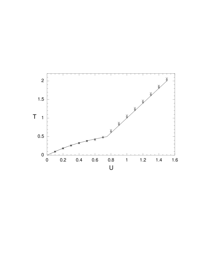
Figure 1: The full line gives the canonical theoretical caloric curve (temperature $T$ $vs$ energy density $U$) for long range rotators compared with the microcanonical simulation of a threedimensional simple cubic lattice for three different $\alpha$ values: $0.75$ (open circles), $1.5$ (diamonds) and $2.25$ (crosses). Note that in spite of the size of the system, still not very large (side with $7$ lattice sites), the results already follow very well the theoretical curve.

3 Conclusions

Going back to the beginning of our discussion: it is now clear that model (2) completely reduces to model (1) for $\alpha=0$. In model (1) the range of the interactions is infinite; each rotator interacts with all the others and with the same intensity. To get a well defined TL it is sufficient to divide $V$ in (1) by $N$, the total numbers of rotators. It is then possible to compute caloric and magnetization curves [3]; the spatial arrangement of the rotators has no effect on them since the intensity of the interaction is the same for each couple of rotators. In this work we have shown that, when considering model (2), it is possible to take into account the spatial $d$-dimensional arrangement of the rotators and the decaying of their mutual interaction through a factor $\tilde{N}$, which is computable for any periodic lattice and any $\alpha<d$. Dividing by $\tilde{N}$ the potential energy in (2), the model gets a well defined TL and it is possible to compute state curves which become those of the HMF model with a proper normalization of the constant $A$ in (17). The HMF ($\alpha=0$) model has revealed peculiar equilibrium and nonequilibrium properties [2], namely: ensemble inequivalence, metastability, collective oscillations, anomalous diffusion and interesting chaotic properties, both in the ferromagnetic and antiferromagnetic case. On the basis of the thermodynamical equivalence here established it would be interesting to investigate the $\alpha$ dependence of all these properties. The study of the Lyapounov exponents in [4] is the first in this direction.

4 Aknowledgments

A. G. warmly thanks C. Tsallis for having suggested the study of the long range interacting rotators.

References

- [1] D. Ruelle, Statistical mechanics: rigorous results, (Addison-Wesley, New York 1989).
- [2] V. Latora, A. Rapisarda, and S. Ruffo, cond-mat/0001010, to appear in Prog. Theor. Phys. Supplement.
- [3] M. Antoni and S. Ruffo, Phys. Rev. E 52, 2361 (1995).
- [4] C. Anteneodo and C. Tsallis, Phys. Rev. Lett. 80, 5313 (1998).
- [5] F. Tamarit and C. Anteneodo, Phys. Rev. Lett. 84, 208 (2000).
- [6] H. Yoshida, Phys. Lett. A 150, 262 (1990).