Hamiltonian dynamics and geometry of phase transitions in classical XY models

Abstract

The Hamiltonian dynamics associated to classical, planar, Heisenberg XY models is investigated for two- and three-dimensional lattices. Besides the conventional signatures of phase transitions, here obtained through time averages of thermodynamical observables in place of ensemble averages, qualitatively new information is derived from the temperature dependence of Lyapunov exponents. A Riemannian geometrization of newtonian dynamics suggests to consider other observables of geometric meaning tightly related with the largest Lyapunov exponent. The numerical computation of these observables - unusual in the study of phase transitions - sheds a new light on the microscopic dynamical counterpart of thermodynamics also pointing to the existence of some major change in the geometry of the mechanical manifolds at the thermodynamical transition. Through the microcanonical definition of the entropy, a relationship between thermodynamics and the extrinsic geometry of the constant energy surfaces $\Sigma_{E}$ of phase space can be naturally established. In this framework, an approximate formula is worked out, determining a highly non-trivial relationship between temperature and topology of the $\Sigma_{E}$. Whence it can be understood that the appearance of a phase transition must be tightly related to a suitable major topology change of the $\Sigma_{E}$. This contributes to the understanding of the origin of phase transitions in the microcanonical ensemble.

I Introduction

The present paper deals with the study of the microscopic Hamiltonian dynamical phenomenology associated to thermodynamical phase transitions. This general subject is addressed in the special case of planar, classical Heisenberg XY models in two and three spatial dimensions. A preliminary presentation of some of the results and ideas contained in this paper has been already given in [4].

There are several reasons to tackle the Hamiltonian dynamical counterpart of phase transitions. On the one hand, we might wonder whether our knowledge of the already wide variety of dynamical properties of Hamiltonian systems can be furtherly enriched by considering the dynamical signatures, if any, of phase transitions. On the other hand, it is a-priori conceivable that also the theoretical investigation of the phase transition phenomena could benefit of a direct investigation of the natural microscopic dynamics. In fact, from a very general point of view, we can argue that in those times where microscopic dynamics was completely unaccessible to any kind of investigation, statistical mechanics has been invented just to replace dynamics. During the last decades, the advent of powerful computers has made possible, to some extent, a direct access to microscopic dynamics through the so called molecular dynamical simulations of the statistical properties of ”macroscopic” systems.

Molecular dynamics can be either considered as a mere alternative to Monte Carlo methods in practical computations, or it can be also seen as a possible link to concepts and methods (those of nonlinear Hamiltonian dynamics) that could deepen our insight about phase transitions. In fact, by construction, the ergodic invariant measure of the Monte Carlo stochastic dynamics, commonly used in numerical statistical mechanics, is the canonical Gibbs distribution, whereas there is no general result that guarantees the ergodicity and mixing of natural (Hamiltonian) dynamics. Thus, the general interest for any contribution that helps in clarifying under what conditions equilibrium statistical mechanics correctly describes the average properties of a large collection of particles, safely replacing their microscopic dynamical description.

Actually, as it has been already shown and confirmed by the results reported below, there are some intrinsically dynamical observables that clearly signal the existence of a phase transition. Notably, Lyapunov exponents appear as sensitive measurements for phase transitions. They are also probes of a hidden geometry of the dynamics, because Lyapunov exponents depend on the geometry of certain “mechanical manifolds” whose geodesic flows coincide with the natural motions. Therefore, a peculiar energy – or temperature – dependence of the largest Lyapunov exponent at a phase transition point also reflects some important change in the geometry of the mechanical manifolds.

As we shall discuss throughout the present paper, also the topology of these manifolds has been discovered to play a relevant role in the phase transition phenomena (PTP).

Another strong reason of interest for the Hamiltonian dynamical counterpart of PTP is related to the equivalence problem of statistical ensembles. Hamiltonian dynamics has its most natural and tight relationship with microcanonical ensemble. Now, the well known equivalence among all the statistical ensembles in the thermodynamic limit is valid in general in the absence of thermodynamic singularities, i.e. in the absence of phase transitions. This is not a difficulty for statistical mechanics as it might seem at first sight [5], rather, this is a very interesting and intriguing point.

The inequivalence of canonical and microcanonical ensembles in presence of a phase transition has been analytically shown for a particular model by Hertel and Thirring [6], it is mainly revealed by the appearance of negative values of the specific heat and has been discussed by several authors [7, 8].

The microcanonical description of phase transitions seems also to offer many advantages in tackling first order phase transitions [9], and seems considerably less affected by finite-size scaling effects with respect to the canonical ensemble description [10]. This non-equivalence problem, together with certain advantages of the microcanonical ensemble, strenghtens the interest for the Hamiltonian dynamical counterpart of PTP. Let us briefly mention the existing contributions in the field.

Butera and Caravati [11], considering an XY model in two dimensions, found that the temperature dependence of the largest Lyapunov exponent changes just near the critical temperature $T_{c}$ of the Kosterlitz-Thouless phase transition. Other interesting aspects of the Hamiltonian dynamics of the XY model in two dimensions have been extensively considered in [12], where a very rich phenomenology is reported. Recently, the behaviour of Lyapunov exponents has been studied in Hamiltonian dynamical systems: i) with long-range interactions [13, 14, 15], ii) describing either clusters of particles or magnetic or gravitational models exhibiting phase transitions, iii) in classical lattice field theories with $O(1)$, $O(2)$ and $O(4)$ global symmetries in two and three space dimensions [16, 17], iv) in the XY model in two and three space dimensions [4], v) in the ”$\Theta$ - transition” of homopolymeric chains [18]. The pattern of $\lambda(T)$ close to the critical temperature $T_{c}$ is model-dependent. The behaviour of Lyapunov exponents near the transition point has been considered also in the case of first- order phase transitions [19, 20]. It is also worth mentioning the very intriguing result of Ref.[21], where a glassy transition is accompanied by a sharp jump of $\lambda(T)$.

$\lambda(T)$ always detects a phase transition and, even if its pattern close to the critical temperature $T_{c}$ is model-dependent, it can be used as an order parameter – of dynamical origin – also in the absence of a standard order parameter (as in the case of the mentioned ”$\Theta$-transition” of homopolymers and of the glassy transition in amorphous materials). This appears of great prospective interest also in the light of recently developed analytical methods to compute Lyapunov exponents (see Section IV).

Among Hamiltonian models with long-range interactions exhibiting phase transitions, the most extensively studied is the mean-field XY model [14, 22, 23, 24], whose equilibrium statistical mechanics is exactly described, in the thermodynamic limit, by mean-field theory [14]. In this system, the theoretically predicted temperature dependence of the largest Lyapunov exponent $\lambda$ displays a non-analytic behavior at the phase transition point.

The aims of the present paper are

• to investigate the dynamical phenomenology of Kosterlitz-Thouless and of second order phase transitions in the $2d$ and $3d$ classical Heisenberg XY models respectively;

• to highlight the microscopic dynamical counterpart of phase transitions through the temperature dependence of the Lyapunov exponents, also providing some physical interpretation of abstract quantities involved in the geometric theory of chaos (in particular among vorticity, Lyapunov exponents and sectional curvatures of configuration space);

• to discuss the hypothesis that phase transition phenomena could be originated by suitable changes in the topology of the constant energy hypersurfaces of phase space, therefore hinting to a mathematical characterization of phase transitions in the microcanonical ensemble.

The paper is organized as follows: Sections $II$ and $III$ are devoted to the dynamical investigation of the $2d$ and $3d$ XY models respectively. In Section $IV$ the geometric description of chaos is considered, with the analytic derivation of the temperature dependence of the largest Lyapunov exponent, the geometric signatures of a second-order phase transition and the topological hypothesis. Section $V$ contains a presentation of the relationship between the extrinsic geometry and topology of the energy hypersurfaces of phase space and thermodynamics; the results of some numeric computations are also reported. Finally, Section $VI$ is devoted to summarize the achievements reported in the present paper and to discuss their meaning.

II $2d$ XY model

We considered a system of planar, classical “spins” (in fact rotators) on a square lattice of $N=n\times n$ sites, and interacting through the ferromagnetic interaction $V=-\sum_{\langle i,j\rangle}J{\bf S}_{i}\cdot{\bf S}_{j}$ (where $|{\bf S}_{i}|=1)$. The addition of standard, i.e. quadratic, kinetic energy term leads to the following choice of the Hamiltonian

$$H=\sum_{i,j=1}^{n}\left\{\frac{p_{i,j}^{2}}{2}+J[2-\cos(q_{i+1,j}-q_{i,j})-\cos(q_{i,j+1}-q_{i,j})]\right\}~{}~{},$$ (1)

where $q_{i,j}$ are the angles with respect to a fixed direction on the reference plane of the system. In the usual definition of the XY model both the kinetic term and the constant term $2JN$ are lacking; however, their contribution does not modify the thermodynamic averages (because they usually depend only on the configurational partition function, $Z_{C}=\int\prod_{i=1}^{N}dq_{i}\exp[-\beta V(q)]$, the momenta being trivially integrable when the kinetic energy is quadratic). Thus, as we tackle classical systems, the choice of a quadratic kinetic energy term is natural because it corresponds to $\frac{1}{2}\sum_{i=1}^{N}|{\bf\dot{S}}_{i}|^{2}$, written in terms of the momenta $p_{i,j}$ canonically conjugated to the lagrangian coordinates $q_{i,j}$. The constant term $2JN$ is introduced to make the low energy expansion of Eq. (1) coincident with the Hamiltonian of a system of weakly coupled harmonic oscillators.

The theory predicts for this model a Kosterlitz-Thouless phase transition occurring at a critical temperature estimated around $T_{c}\sim J$. Many Monte Carlo simulations of this model have been done in order to check the predictions of the theory. Among them, we quote those of Tobochnik and Chester [25] and of Gupta and Baillie [26] which, on the basis of accurate numerical analysis, confirmed the predictions of the theory and fixed the critical temperature at $T_{c}=0.89$ ($J=1$).

The analysis of the present work is based on the numerical integration of the equations of motion derived from Hamiltonian (1). The numerical integration is performed by means of a bilateral, third order, symplectic algorithm [27], and it is repeated at several values of the energy density $\epsilon=E/N$ ($E$ is the total energy of the system which depends upon the choice of the initial conditions). While the Monte Carlo simulations perform statistical averages in the canonical ensemble, Hamiltonian dynamics has its statistical counterpart in the microcanonical ensemble. Statistical averages are here replaced by time averages of relevant observables. In this perspective, from the microcanonical definition of temperature $1/T=\partial S/\partial E$, where $S$ is the entropy, two definitions of temperature are available: $T=\frac{2}{N}\langle K\rangle$ (where $K$ is the kinetic energy per degree of freedom), if $S=\log\int\prod_{i=1}^{N}dq_{i}dp_{i}\Theta(H(p,q)-E)$, where $\Theta(\cdot)$ is the Heaviside step function, and $\tilde{T}=\left[\left(\frac{N}{2}-1\right)\langle K^{-1}\rangle\right]^{-1}$, if $S=\log\int\prod_{i=1}^{N}dq_{i}dp_{i}\delta(H(p,q)-E)$ [28]. $T$ (or $\tilde{T}$) are numerically determined by measuring the time average of the kinetic energy $K$ per degree of freedom (or its inverse), i.e. $T=\lim_{t\rightarrow\infty}\frac{2}{N}\frac{1}{t}\int_{0}^{t}d\tau K(\tau)$ (and similarly for $\tilde{T}$). There is no appreciable difference in the outcomes of the computations of temperature according to these two definitions.

A Dynamical analysis of thermodynamical observables

1 Order parameter

The order parameter for a system of planar “spins” whose Hamiltonian is invariant under the action of the group $O(2)$, is the bidimensional vector

$${\bf M}=(\sum_{i,j=1}^{n}{\bf S}^{x}_{i,j},\sum_{i,j=1}^{n}{\bf S}^{y}_{i,j})\equiv(\sum_{i,j=1}^{n}\cos q_{i,j},\sum_{i,j=1}^{n}\sin q_{i,j}),$$ (2)

which describes the mean spin orientation field. After the Mermin-Wagner theorem, we know that no symmetry-breaking transition can occur in one and two dimensional systems with a continuous symmetry and nearest-neighbour interactions. This means that, at any non-vanishing temperature, the statistical average of the total magnetization vector is necessarily zero in the thermodynamic limit. However, a vanishing magnetization is not necessarily expected when computed by means of Hamiltonian dynamics at finite $N$. In fact, statistical averages are equivalent to averages computed through suitable markovian Monte Carlo dynamics that a-priori can reach any region of phase space, whereas in principle a true ergodicity breaking is possible in the case of differentiable dynamics. Also an ”effective” ergodicity breaking of differentiable dynamics is possible, when the relaxation times – of time to ensemble averages – are very fastly increasing with $N$ [29].

This model has two integrable limits: coupled harmonic oscillators and free rotators, at low and high temperatures respectively. Hereafter, $T$ is meant in units of the coupling constant $J$.

For a lattice of $N=10\times 10$ sites, Figure 1 shows that at low temperatures ($T<0.5$)– being the system almost harmonic – we can observe a persistent memory of the total magnetization associated with the initial condition, which, on the typical time scales of our numeric simulations ($10^{6}$ units of proper time), looks almost frozen.

By raising the temperature above a first threshold $T_{0}\simeq 0.6$, the total magnetization vector – observed on the same time scale – starts rotating on the plane where it is confined. A further increase of the temperature induces a faster rotation of the magnetization vector together with a slight reduction of its average modulus.

At temperatures slightly greater than $1$, we observe that already at $N=10\times 10$ a random variation of the direction and of the modulus of the vector ${\bf M}(t)$ sets in.

At $T>1.2$, we observe a fast relaxation and, at high temperatures ($T\simeq 10$), a sort of saturation of chaos.

At a first glance, the results reported in Fig. 1 could suggest the presence of a phase transition associated with the breaking of the $O(2)$ symmetry. In fact, having in mind the Landau theory, the ring-shaped distribution of the instantaneous magnetization shown by Fig. 1 is the typical signature of an $O(2)$-broken symmetry phase and the spot-like patterns around zero are proper to the unbroken symmetry phase.

The apparent contradiction of these results with the Mermin-Wagner theorem is resolved by checking whether the observed phenomenology is stable with $N$. Thus, some simulations have been performed at larger values of $N$. At any temperature, we found that the average modulus $\langle|{\bf M}(t)|\rangle_{t}$ of the vector ${\bf M}(t)$, computed along the trajectory, systematically decreases by increasing $N$. However, for temperatures lower than $T_{0}$, the $N$-dependence of the order parameter is very weak, whereas, for temperatures greater than $T_{0}$, the $N$-dependence of the order parameter is rather strong. In Fig. 2 two extreme cases ($N=10\times 10$ and $N=200\times 200$) are shown for $T=0.74$. The systematic trend of $\langle|{\bf M}(t)|\rangle$ toward smaller values at increasing $N$ is consistent with its expected vanishing in the limit $N\rightarrow\infty$.

At $T=1$, Fig. 3 shows that, when the lattice dimension is greater than $50\times 50$, ${\bf M}(t)$ displays random variations both in direction (in the interval [0,$2\pi$]) and in modulus (between zero and a value which is smaller at larger $N$).

2 Specific heat

By means of the recasting of a standard formula which relates the average fluctuations of a generic observable computed in canonical and microcanonical ensembles [30], and by specializing it to the kinetic energy fluctuations, one obtains a microcanonical estimate of the canonical specific heat

$$c_{V}(T)=\frac{C_{V}}{N}\rightarrow\cases{c_{V}(\epsilon)=\displaystyle{\frac{k_{B}d}{2}\left[1-\frac{Nd}{2}\frac{\langle K^{2}\rangle-\langle K\rangle^{2}}{\langle K\rangle^{2}}\right]^{-1}}~{}~{},\cr T=T(\epsilon)\cr}$$ (3)

where $d$ is the number of degrees of freedom for each particle. Time averages of the kinetic energy fluctuations computed at any given value of the energy density $\epsilon$ yield $C_{V}(T)$, according to its parametric definition in Eq.(3).

¿From the microcanonical definition $1/C_{V}=\partial T(E)/\partial E$ of the constant volume specific heat, a formula can be worked out [28], which is exact at any value of $N$ (at variance with the expression (3)). It reads

$$c_{V}=\frac{C_{V}}{N}=[N-(N-2)\langle K\rangle\langle K^{-1}\rangle]^{-1}$$ (4)

and it is the natural expression to be used in Hamiltonian dynamical simulations of finite systems.

The numerical simulations of the Hamiltonian dynamics of the $2d$ XY model – computed with both Eqs.(3) and (4) – yield a cuspy pattern for $c_{V}(T)$ peaked at $T\simeq 1$ (Fig. 4). This is in good agreement with the outcomes of canonical Monte Carlo simulations reported in Ref. [25, 26], where a pronounced peak of $c_{V}(T)$ was detected at $T\simeq 1.02$.

By varying the lattice dimensions, the peak height remains constant, in agreement with the absence of a symmetry-breaking phase transition.

3 Vorticity

Another thermodynamic observable which can be studied is the vorticity of the system. Let us briefly recall that if the angular differences of nearby “spins” are small, we can suppose the existence of a continuum limit function $\theta({\bf r})$ that conveniently fits a given spatial configuration of the system. Spin waves correspond to regular patterns of $\theta({\bf r})$, whereas the appearance of a singularity in $\theta({\bf r})$ corresponds to a topological defect, or a vortex, in the “spin” configuration. When such a defect is present, along any closed path ${\cal C}$ that contains the centre of the defect, one has

$$\oint_{\cal C}\nabla\theta({\bf r})\cdot d{\bf r}=2\pi q~{},~{}~{}~{}~{}q=0,\pm 1,\pm 2,\dots$$ (5)

indicating the presence of a vortex whose intensity is $q$. For a lattice model with periodic boundary conditions, there is an equal number of vortices and antivortices (i.e. vortices rotating in opposite directions). Thus, the vorticity of our model can be defined as the mean total number of equal sign vortices per unit volume. In order to compute the vorticity ${\cal V}$ as a function of temperature, we have averaged the number of positive vortices along the numerical phase space trajectories. On the lattice, ${\bf r}$ is replaced by the multi-index ${\bf i}$ and $\nabla_{\mu}\theta_{i}=q_{{\bf i}+\mu}-q_{\bf i}$, then the number of elementary vortices is counted: the discretized version of $\oint_{\square}\nabla\theta\cdot d{\bf r}=1$ amounts to one elementary vortex on a plaquette. Thus ${\cal V}$ is obtained by summing over all the plaquettes.

Our results are in agreement with the values obtained by Tobochnik and Chester [25] by means of Monte Carlo simulations with $N=60\times 60$.

As shown in Fig. 5, on the $10\times 10$ lattice, the first vortex shows up at $T\sim 0.6$ and on the $40\times 40$ lattice at $T\sim 0.5$, when the system changes its dynamical behavior, increasing its chaoticity (see next Subsection). At lower temperatures, vortices are less probable, due to the fact that the formation of vortex has a minimum energy cost. Below $T\sim 1$, the vortex density steeply grows with a power law ${\cal V}(T)\sim T^{10}$. The growth of ${\cal V}$ then slows down, until the saturation is reached at $T\sim 10$.

B Lyapunov exponents and chaoticity

The values of the largest Lyapunov exponent $\lambda_{1}$ have been computed using the standard tangent dynamics equations [see Eqs. (11) and (60)], and are reported in Fig. 6.

Below $T\simeq 0.6$, the dynamical behavior is nearly the same as that of harmonic oscillators and the excitations of the system are only “spin-waves”.

In the interval $[0.,0.6]$, the observed temperature dependence $\lambda_{1}(T)\sim T^{2}$ is equivalent to the $\lambda_{1}(\epsilon)\sim\epsilon^{2}$ dependence (since at low temperature $T(\epsilon)\propto\epsilon$), already found – analytically and numerically – in the quasi-harmonic regime of other systems and characteristic of weakly chaotic dynamics [31].

Above $T\simeq 0.6$, vortices begin to form and correspondingly the largest Lyapunov exponent signals a ”qualitative” change of the dynamics through a steeper increase vs. $T$.

At $T\simeq 0.9$, where the theory predicts a Kosterlitz - Thouless phase transition, $\lambda_{1}(T)$ displays an inflection point.

Finally, at high temperatures, the power law $\lambda_{1}(T)\sim T^{-1/6}$ is found.

III $3d$ XY model

In order to extend the dynamical investigation to the case of second-order phase transitions, we have studied a system described by an Hamiltonian having at the same time the main characteristics of the $2d$ model and the differences necessary to the appearance of a spontaneous symmetry-breaking below a certain critical temperature. The model we have chosen is such that the spin rotation is constrained on a plane and only the lattice dimension has been increased, in order to elude the “no go” conditions of the Mermin-Wagner theorem. This is simply achieved by tackling a system defined on a cubic lattice of $N=n\times n\times n$ sites and described by the Hamiltonian

$$H = \sum_{i,j,k=1}^{n}\{\frac{p_{i,j,k}^{2}}{2}+J[3-\cos(q_{i+1,j,k}-q_{i,j,k})-$$ (6)

$$- \cos(q_{i,j+1,k}-q_{i,j,k})-\cos(q_{i,j,k+1}-q_{i,j,k})]\}~{}~{}.$$ (7)

A Dynamical analysis of thermodynamical observables

The basic thermodynamical phenomenology of a second-order phase transition is characterized by the existence of equilibrium configurations that make the order parameter bifurcating away from zero at some critical temperature $T_{c}$ and by a divergence of the specific heat $c_{V}(T)$ at the same $T_{c}$. Therefore, this is the obvious starting point for the Hamiltonian dynamical approach.

1 Order parameter

Below a critical value of the temperature, the symmetry-breaking in a system invariant under the action of the $O(2)$ group, appears as the selection – by the average magnetization vector of Eq. (2)– of a preferred direction among all the possible, energetically equivalent choices. By increasing the lattice dimension, the symmetry breaking is therefore characterized by a sort of simultaneous ”freezing” of the direction of the order parameter ${\bf M}$ and of the convergence of its modulus to a non-zero value.

Figure 7 shows that in the $3d$ lattice, at $T<2$, i.e. in the broken-symmetry phase (as we shall see in the following), the dynamical simulations yield a thinner spread of the longitudinal fluctuations by increasing $N$ – that is, $|{\bf M}|$ oscillates by exhibiting a trend to converge to a non-zero value – and that the transverse fluctuations damp, “fixing” the direction of the oscillations. This direction depends on the initial conditions.

Moreover, the dynamical analysis provides us with a better detail than a simple distinction between regular and chaotic dynamics. In fact, it is possible to distinguish between three different dynamical regimes (Fig. 8).

At low temperatures, up to $T\simeq 0.8$, one observes the persistency of the initial direction and of an equilibrium value of the modulus $|{\bf M}|$ close to one.

At $0.8<T<2.2$, one observes transverse oscillations, whose amplitude increases with temperature.

At $T>2.2$, the order parameter exhibits the features typical of an unbroken symmetry phase. In fact, it displays fluctuations peaked at zero, whose dispersion decreases by increasing the temperature (bottom of Fig. 8) and, at a given temperature, by increasing the lattice volume (Fig. 9a,b).

We can give an estimate of the order parameter by evaluating the average of the modulus $\langle|{\bf M}(t)|\rangle=\rho(T)$. At $T<2.2$, the $N$-dependence is given mainly by the rotation of the vector, while the longitudinal oscillations are moderate, as shown in Fig. 10. At temperatures above $T\simeq 2.2$, we observe the squeezing of $\rho(T)$ to a small value.

The existence of a second order phase transition can be recognized by comparing the temperature behavior and the $N$-dependence of the thermodynamic observables computed for the $2d$ and the $3d$ models. Both systems exhibit the rotation of the magnetization vector and small fluctuations of its modulus when they are considered on small lattices. In the $2d$ model the average modulus of the order parameter is theoretically expected to vanish logarithmically with $N$, what seems qualitatively compatible with the weak $N$ dependence shown in Fig. 2, whereas in the $3d$ model we observe a stability with $N$ of $\langle|{\bf M}|\rangle$, suggesting the convergence to a non-zero value of the order parameter also in the limit $N\rightarrow\infty$, as shown in Fig. 7.

$T\simeq 2.2$ is an approximate value of the critical temperature $T_{c}$ of the second-order phase transition. This value will be refined in the following Subsection. No finite-size scaling analysis has been performed for two different reasons: i) our main concern is a qualitative phenomenological analysis of the Hamiltonian dynamics of phase transitions rather than a very accurate quantitative analysis, ii) finite-size effects are much weaker in the microcanonical ensemble than in the canonical ensemble [10].

2 Specific heat

As in the $2d$ model, numerical simulations of the Hamiltonian dynamics have been performed with both Eqs.(3) and (4). The outcomes show a cusplike pattern of the specific heat, whose peak makes possible a better determination of the critical temperature. By increasing the lattice dimension up to $N=15\times 15\times 15$, the cusp becomes more pronounced, at variance with the case of the $2d$ model. Fig. 11 shows that this occurs at the temperature $T_{c}\simeq 2.17$.

3 Vorticity

The definition of the vorticity in the $3d$ case is not a simple extension of the $2d$ case. Vortices are always defined on a plane and if all the “spins” could freely move in the three-dimensional space, the concept of vortices would be meaningless. For the $3d$ planar (anisotropic) model considered here, vortices can be defined and studied on two-dimensional subspaces of the lattice. The variables $q_{i,j,k}$ do not contain any information about the position of the plane where the reference direction to measure the angles $q_{i,j,k}$ is assigned. Dynamics is completely independent of this choice, which has no effect on the Hamiltonian. Moreover, as the Hamiltonian is symmetric with respect to the lattice axes, the three coordinate-planes are equivalent. This equivalence implies that vortices can contemporarily exist on three orthogonal planes. Though the usual pictorial representation of a vortex can hardly be maintained, its mathematical definition is the same as in the $2d$ lattice case. Hence three vorticity functions exist and their average values - at a given temperature - should not differ, what is actually confirmed by numerical simulations.

The vorticity function vs. temperature is plotted in Fig. 12. On a lattice of $10\times 10\times 10$ spins, the first vortex is observed at $T\simeq 0.8$. The growth of the average density of vortices is very fast up to the critical temperature, above which the saturation is reached.

B Lyapunov exponents and symmetry-breaking phase transition

A quantitative analysis of the dynamical chaoticity is provided by the temperature dependence of the largest Lyapunov exponent.

Figure 13 shows the results of this computation. At low temperatures, in the limit of quasi-harmonic oscillators, the scaling law is again found to be $\lambda_{1}(T)\sim T^{2}$ and, at high temperatures, the scaling law is again $\lambda_{1}(T)\sim T^{-1/6}$, as in the $2d$ case. In the temperature range intermediate between $T\simeq 0.8$ and $T_{c}\simeq 2.17$, there is a linear growth of $\lambda_{1}(T)$. At the critical temperature, the Lyapunov exponent exhibits an angular point. This makes a remarkable difference between this system undergoing a second order phase transition and its $2d$ version, undergoing a Kosterlitz- Thouless transition. In fact, the analysis of the $2d$ model has shown a mild transition between the different regimes of $\lambda_{1}(T)$ (inset of Fig. 12), whereas in the $3d$ model this transition is sharper (inset of Fig. 13).

We have also computed the temperature dependence of the largest Lyapunov exponent of Markovian random processes which replace the true dynamics on the energy surfaces $\Sigma_{E}$ (see Appendix). The results are shown in Fig. 14. The dynamics is considered strongly chaotic in the temperature range where the patterns $\lambda_{1}(T)$ are the same for both random and differentiable dynamics, i.e. when differentiable dynamics mimics, to some extent, a random process. The dynamics is considered weakly chaotic when the value $\lambda_{1}$ resulting from random dynamics is larger than the value $\lambda_{1}$ resulting from differentiable dynamics. The transition from weak to strong chaos is quite abrupt. Figure 14 shows that the pattern of the largest Lyapunov exponent computed by means of the random dynamics reproduces that of the true Lyapunov exponent at temperatures $T\geq T_{c}$. This means that the setting in of strong thermodynamical disorder corresponds to the setting in of strong dynamical chaos. The “window” of strong chaoticity starts at $T_{c}$ and ends at $T\sim 10$. The existence of a second transition from strong to weak chaos is due to the existence, for $T\rightarrow\infty$, of the second integrable limit (of free rotators), whence chaos cannot remain strong at any $T>T_{c}$.

IV Geometry of dynamics and phase transitions

Let us briefly recall that the geometrization of the dynamics of $N$-degrees-of-freedom systems defined by a Lagrangian ${\cal L}=K-V$, in which the kinetic energy is quadratic in the velocities: $K=\frac{1}{2}a_{ij}\dot{q}^{i}\dot{q}^{j}~{}$, stems from the fact that the natural motions are the extrema of the Hamiltonian action functional ${\cal S}_{H}=\int{\cal L}\,dt$, or of the Maupertuis’ action ${\cal S}_{M}=2\int K\,dt$. In fact, also the geodesics of Riemannian and pseudo-Riemannian manifolds are the extrema of a functional, the arc-length $\ell=\int ds$, with $ds^{2}={g_{ij}dq^{i}dq^{j}}$. Hence, a suitable choice of the metric tensor allows for the identification of the arc-length with either ${\cal S}_{H}$ or ${\cal S}_{M}$, and of the geodesics with the natural motions of the dynamical system. Starting from ${\cal S}_{M}$, the “mechanical manifold” is the accessible configuration space endowed with the Jacobi metric [32]

$$(g_{J})_{ij}=[E-V(q)]\,a_{ij}~{}~{},$$ (8)

where $V(q)$ is the potential energy and $E$ is the total energy. A description of the extrema of Hamilton’s action ${\cal S}_{H}$ as geodesics of a “mechanical manifold” can be obtained using Eisenhart’s metric [33] on an enlarged configuration spacetime ($\{q^{0}\equiv t,q^{1},\ldots,q^{N}\}$ plus one real coordinate $q^{N+1}$), whose arc-length is

$$ds^{2}=-2V(\{q\})(dq^{0})^{2}+a_{ij}dq^{i}dq^{j}+2dq^{0}dq^{N+1}~{}~{}.$$ (9)

The manifold has a Lorentzian structure and the dynamical trajectories are those geodesics satisfying the condition $ds^{2}=Cdt^{2}$, where $C$ is a positive constant. In the geometrical framework, the (in)stability of the trajectories is the (in)stability of the geodesics, and it is completely determined by the curvature properties of the underlying manifold according to the Jacobi equation [32, 34]

$$\frac{\nabla^{2}\xi^{i}}{ds^{2}}+R^{i}_{~{}jkm}\frac{dq^{j}}{ds}\xi^{k}\frac{dq^{m}}{ds}=0~{}~{},$$ (10)

whose solution $\xi$, usually called Jacobi or geodesic variation field, locally measures the distance between nearby geodesics; $\nabla/ds$ stands for the covariant derivative along a geodesic and $R^{i}_{~{}jkm}$ are the components of the Riemann curvature tensor. Using the Eisenhart metric (9), the relevant part of the Jacobi equation (10) is [31]

$$\frac{d^{2}\xi^{i}}{dt^{2}}+R^{i}_{~{}0k0}\xi^{k}=0~{}~{},~{}~{}~{}~{}i=1,\dots,N$$ (11)

where the only non-vanishing components of the curvature tensor are $R_{0i0j}=\partial^{2}V/\partial q_{i}\partial q_{j}$. Equation (11) is the tangent dynamics equation, which is commonly used to measure Lyapunov exponents in standard Hamiltonian systems. Having recognized its geometric origin, it has been devised in Ref.[31] a geometric reasoning to derive from Eq.(11) an effective scalar stability equation that, independently of the knowledge of dynamical trajectories, provides an average measure of their degree of instability. An intermediate step in this derivation yields

$$\frac{d^{2}\xi^{j}}{dt^{2}}+k_{R}(t)\xi^{j}+\delta K^{(2)}{(t)}\xi^{j}=0~{}~{},$$ (12)

where $k_{R}=K_{R}/N$ is the Ricci curvature along a geodesic defined as $K_{R}=\frac{1}{v^{2}}R_{ij}{\dot{q}^{i}}{\dot{q}^{j}}$, with $v^{2}={\dot{q}^{i}}{\dot{q}_{i}}$ and $R_{ij}=R^{k}_{~{}ikj}$, and $\delta K^{(2)}$ is the local deviation of sectional curvature from its average value [31]. The sectional curvature is defined as $K^{(2)}=R_{~{}ijkl}\xi^{i}\dot{q}^{j}\xi^{k}\dot{q}^{l}/\parallel\xi\parallel^{2}\parallel\dot{q}\parallel^{2}$.

Two simplifying assumptions are made: $(i)$ the ambient manifold is almost isotropic, i.e. the components of the curvature tensor — that for an isotropic manifold (i.e. of constant curvature) are $R_{ijkm}=k_{0}(g_{ik}g_{jm}-g_{im}g_{jk})$, $k_{0}=const$ – can be approximated by $R_{ijkm}\approx k(t)(g_{ik}g_{jm}-g_{im}g_{jk})$ along a generic geodesic $\gamma(t)$; $(ii)$ in the large $N$ limit, the “effective curvature” $k(t)$ can be modeled by a gaussian and $\delta$-correlated stochastic process. Hence, one derives an effective stability equation, independent of the dynamics and in the form of a stochastic oscillator equation [31],

$$\frac{d^{2}\psi}{dt^{2}}+[k_{0}+\sigma_{k}\eta(t)]\,\psi=0~{}~{},$$ (13)

where $\psi^{2}\propto|\xi|^{2}$. The mean $k_{0}$ and variance $\sigma_{k}$ of $k(t)$ are given by $k_{0}={\langle K_{R}\rangle}/{N}$ and $\sigma^{2}_{k}={\langle(K_{R}-\langle K_{R}\rangle)^{2}\rangle}/{N}$, respectively, and the averages $\langle\cdot\rangle$ are geometric averages, i.e. integrals computed on the mechanical manifold. These averages are directly related with microcanonical averages, as it will be seen at the end of Section V. $\eta(t)$ is a gaussian $\delta$-correlated random process of zero mean and unit variance.

The main source of instability of the solutions of Eq.(13), and therefore the main source of Hamiltonian chaos, is parametric resonance, which is activated by the variations of the Ricci curvature along the geodesics and which takes place also on positively curved manifolds [35]. The dynamical instability can be enhanced if the geodesics encounter regions of negative sectional curvatures, such that $k_{R}+\delta K^{(2)}<0$, as it is evident from Eq. (12).

In the case of Eisenhart metric, it is $K_{R}\equiv\Delta V=\sum_{i=1}^{N}({\partial^{2}V}/{\partial q_{i}^{2}})$ and $K^{(2)}=R_{~{}0i0j}\xi^{i}\xi^{j}/\parallel\xi\parallel^{2}\equiv(\partial^{2}V/\partial q^{i}\partial q^{j})\xi^{i}\xi^{j}/\|\xi\|^{2}$. The exponential growth rate $\lambda$ of the quantity $\psi^{2}+\dot{\psi}^{2}$ of the solutions of Eq. (13), is therefore an estimate of the largest Lyapunov exponent that can be analytically computed. The final result reads [31]

$$\lambda=\frac{\Lambda}{2}-\frac{2k_{0}}{3\Lambda}\,,~{}~{}\Lambda=\left(2\sigma_{k}^{2}\tau+\sqrt{\frac{64k_{0}^{3}}{27}+4\sigma_{k}^{4}\tau^{2}}~{}\right)^{\frac{1}{3}}~{},$$ (14)

where $\tau=\pi\sqrt{k_{0}}/(2\sqrt{k_{0}(k_{0}+\sigma_{k})}+\pi\sigma_{k})$; in the limit $\sigma_{k}/k_{0}\ll 1$ one finds $\lambda\propto\sigma_{k}^{2}~{}$.

A Signatures of phase transitions from geometrization of dynamics

In the geometric picture, chaos is mainly originated by the parametric instability activated by the fluctuating curvature felt by geodesics, i.e. the fluctuations of the (effective) curvature are the source of the instability of the dynamics. On the other hand, as it is witnessed by the derivation of Eq. (13) and by the equation itself, a statistical-mechanical-like treatment of the average degree of chaoticity is made possible by the geometrization of the dynamics. The relevant curvature properties of the mechanical manifolds are computed, at the formal level, as statistical averages, like other thermodynamic observables. Thus, we can expect that some precise relationship may exist between geometric, dynamic and thermodynamic quantities. Moreover, this implies that phase transitions should correspond to peculiar effects in the geometric observables.

In the particular case of the $2d$ XY model, the microcanonical average kinetic energy $\langle K\rangle$ and the average Ricci curvature $\langle K_{R}\rangle$ computed with the Eisenhart metric are linked by the equation

$$K_{R}=\left\langle\sum_{i,j=1}^{N}\frac{\partial^{2}V}{\partial^{2}q_{i,j}}\right\rangle=2J\sum_{i,j=1}^{N}\left\langle\cos(q_{i+1,j}-q_{i,j})+\cos(q_{i,j+1}-q_{i,j})\right\rangle=2(J-\langle V\rangle)~{}~{},$$ (15)

so that

$$H=N\epsilon=\langle K\rangle+\langle V\rangle\mapsto\frac{\langle K\rangle}{N}=\epsilon-2J+\frac{1}{2}\frac{\langle K_{R}\rangle}{N}~{}~{}.$$ (16)

Being the temperature defined as $T=2\langle K\rangle/N$ (with $k_{B}=1$) and being $d=1$ (because each spin has only one rotational degree of freedom), from Eq.(3) it follows that

$$c_{V}=\frac{1}{2}\left(1-\frac{1}{2}\frac{\sigma^{2}_{k}/N}{T^{2}}\right)^{-1}.$$ (17)

In the special case of these XY systems, it is possible to link the specific heat and the Ricci curvature by inserting Eq.(16) into the usual expression for the specific heat at constant volume. Thus, one obtains the equation

$$c_{V}=-\frac{1}{2N}\frac{\partial\langle K_{R}\rangle(T)}{\partial T}~{}.$$ (18)

The appearance of a peak in the specific heat function at the critical temperature has to correspond to a suitable temperature dependence of the Ricci curvature.

In the $3d$ model, the potential energy and the Ricci curvature are proportional, according to: $\frac{1}{N}\langle V\rangle=3-\frac{1}{2N}\langle K_{R}\rangle~{}$.

Another interesting point is the relation between a geometric observable and the vorticity function in both models. As already seen in previous sections, the vorticity function is a useful signature of the dynamical chaoticity of the system. From the geometrical point of view, the enhancement of the instability of the dynamics with respect to the parametric instability due to curvature fluctuations, is linked to the probability of obtaining negative sectional curvatures along the geodesics (as discussed for $1d$ XY model in Ref.[31]). In fact, when vortices are present in the system, there will surely be two neighbouring spins with an orientation difference greater than $\pi/2$, such that, if $i,j$ and $i+1,j$ are their coordinates on the lattice, it follows that

$$q_{i+1,j}-q_{i,j}>\frac{\pi}{2}\rightarrow\cos(q_{i+1,j}-q_{i,j})<0~{}.$$ (19)

The sectional curvature relative to the plane defined by the velocity ${\bf v}$ along a geodesic and a generic vector ${\bf\xi}\perp{\bf v}$ is

$$K^{(2)}=\sum_{i,j,k,l=1}^{N}\frac{\partial^{2}V}{\partial q_{i,j}\partial q_{k,l}}\frac{\xi^{i,j}\xi^{k,l}}{\|{\bf\xi}\|^{2}}~{}~{}.$$ (20)

For the $2d$ XY model, it is

$$K^{(2)}=\frac{J}{\|{\bf\xi}\|^{2}}\sum_{i,j=1}^{N}\{\cos(q_{i+1,j}-q_{i,j})[\xi^{i+1,j}-\xi^{i,j}]^{2}+\cos(q_{i,j+1}-q_{i,j})[\xi^{i,j+1}-\xi^{i,j}]^{2}\}~{}.$$ (21)

Thus, a large probability of having a negative value of the cosine of the difference among the directions of two close spins corresponds to a larger probability of obtaining negative values of the sectional curvatures along the geodesics; here for $\xi$ the geodesic separation vector of Eq.(11) is chosen.

In the $3d$ model, the sectional curvature relative to the plane defined by the velocity ${\bf v}$ and a generic vector ${\bf\xi}\perp{\bf v}$ is

$$K^{(2)} = \frac{J}{\|\xi\|^{2}}\sum_{i,j,k=1}^{N}\{\cos(q_{i+1,j,k}-q_{i,j,k})[\xi^{i+1,j,k}-\xi^{i,j,k}]^{2}+$$ (22)

$$+ \cos(q_{i,j+1,k}-q_{i,j,k})[\xi^{i,j+1,k}-\xi^{i,j,k}]^{2}+\cos(q_{i,j,k+1}-q_{i,j,k})[\xi^{i,j,k+1}-\xi^{i,j,k}]^{2}\}$$ (23)

and again the probability of finding negative values of $K^{(2)}$ along a trajectory is limited to the probability of finding vortices.

The mean values of the geometric quantities entering Eq.(13) can be numerically computed by means of Monte Carlo simulations or by means of time averages along the dynamical trajectories. In fact, due to the lack of an explicit expression for the canonical partition function of the system, these averages are not analytically computable. For sufficiently high temperatures, the potential energy becomes negligible with respect to the kinetic energy, and each spin is free to move independently from the others. Thus, in the limit of high temperatures, one can estimate the configurational partition function $Z_{C}=\int_{-\pi}^{\pi}\prod_{\bf i}dq_{\bf i}e^{-\beta V(q)}$ by means of the expression

$$Z_{C} = e^{-2\beta JN}\int_{-\pi}^{\pi}\prod_{i,j=1}^{N}dq_{i,j}\exp\{\beta J\sum_{i,j=1}^{N}[\cos(q_{i+1,j}-q_{i,j})+\cos(q_{i,j+1}-q_{i,j})]\}$$ (24)

$$\sim e^{-2\beta JN}\int_{-\pi}^{\pi}\prod_{i,j=1}^{N}du_{i,j}dv_{i,j}\exp\{\beta J\sum_{i,j=1}^{N}[\cos(u_{i,j})+\cos(v_{i,j})]\}$$ (25)

after the introduction of $u_{i,j}=q_{i+1,j}-q_{i,j}$ and $v_{i,j}=q_{i,j+1}-q_{i,j}$ as independent variables. In this way, some analytical estimates of the average Ricci curvature $k_{0}(T)$ and of its r.m.s. fluctuations $\sigma^{2}_{k}(T)$ have been obtained for the $2d$ model (Fig. 15). For temperatures above the temperature of the Kosterlitz-Thouless transition, these estimates are in agreement with the numerical computations on a $N=10\times 10$ lattice. It is confirmed that Hamiltonian dynamical simulations, already on rather small lattices, are useful to predict, with a good approximation, the thermodynamic limit behavior of relevant observables. Moreover, the good quality of the high temperature estimate gives a further information: at the transition temperature, the correlations among the different degrees of freedom are destroyed, confirming the strong chaoticity of the dynamics.

The same high temperature estimates of $k_{0}(T)$ and $\sigma^{2}_{k}(T)$ have been performed for the $3d$ system. In Fig. 16, the numerical determination of $\sigma^{2}_{k}(T)$ shows the appearance of a very pronounced peak at the phase transition point which is not predicted by the analytic estimate, whereas the average Ricci curvature $k_{0}(T)$ is in agreement with the analytic values of the high temperature estimate, computed by spin decoupling, above the critical temperature, as in the $2d$ model.

B Geometric observables and Lyapunov exponents

We have seen that the largest Lyapunov exponent is sensitive to the phase transition and at the same time we know that it is also related to the average curvature properties of the “mechanical manifolds”. Thus, the geometric observables $k_{0}(T)$ and $\sigma^{2}_{k}(T)$ above considered can be used to estimate the Lyapunov exponents, as well as to detect the phase transition.

In principle, by means of Eq.(14), one can evaluate the largest Lyapunov exponent without any need of dynamics, but simply using global geometric quantities of the manifold associated to the physical system. For $2d$ and $3d$ XY models, fully analytic computations are possible only in the limiting cases of high and low temperatures. Microcanonical averages of $k_{0}$ and $\sigma^{2}_{k}$ at arbitrary $T$ have been numerically computed through time averages. We can call this hybrid method semi-analytic.

In Fig. 17, the results of the semi-analytic prediction of the Lyapunov exponents for the $2d$ model are plotted vs. temperature and compared with the numerical outcomes of the tangent dynamics. As one can see, the prediction formulated on the basis of Eq.(14) underestimates the numerical values given by the tangent dynamics. The semi-analytic prediction can be improved by observing that the replacement of the sectional curvature fluctuation $\delta K^{(2)}$ in Eq.(12) with a fraction of the Ricci curvature [which underlies the derivation of Eq.(13)] underestimates the frequency of occurrence of negative sectional curvatures, which was already the case of the $1d$ XY model [31]. The correction procedure can be implemented by evaluating the probability $P(T)$ of obtaining a negative value of the sectional curvature along a generic trajectory and then by operating the substitution

$$K_{R}(T)\rightarrow\frac{K_{R}(T)}{1+P(T)\alpha}~{}.$$ (26)

The parameter $\alpha$ is a free parameter to be empirically estimated. Its value ranges from $100$ to $200$, without appreciable differences in the final result. It resumes the non trivial information about the more pronounced tendency of the trajectories towards negative sectional curvatures with respect to the predictions of the geometric model describing the chaoticity of the dynamics.

The probability $P(T)$ is estimated through the occurrence along a trajectory of negative values of the sum of the coefficients that appear in the definition of $K^{(2)}$ [Eqs.(21) and (23)]

$$P(T)\sim\frac{\int_{-\pi}^{\pi}\Theta(-\cos(q_{k+1,l}-q_{k,l})-\cos(q_{k,l+1}-q_{k,l}))\exp[-\beta V({\bf q})]\prod_{k,l=1}^{N}dq_{k,l}}{\int_{-\pi}^{\pi}\exp[-\beta V({\bf q})]\prod_{k,l=1}^{N}dq_{k,l}}~{}~{},$$ (27)

averaged over all the sites $\forall k,l\in(1,\ldots,N)$; $\Theta$ is the step function.

Alternatively, owing to the already remarked relation between vorticity and sectional curvature $K^{(2)}$, $P(T)$ can be replaced by the average density of vortices

$$K_{R}(T)\rightarrow\frac{K_{R}(T)}{1+\overline{\alpha}{\cal V}(T)}~{},$$ (28)

where $\overline{\alpha}$ a free parameter. Actually, in the $2d$ model, the two corrections, one given by Eq.(26) with $P(T)$ of Eq. (27), the other given by Eq.(28) with the vorticity function in place of $P(T)$, convey the same information. The semi-analytic predictions of $\lambda_{1}(T)$ with correction are reported in Fig. 17.

In the limits of high and low temperatures, $\lambda_{1}(T)$ can be given the analytic forms $\lambda_{1}(T)\sim T^{-1/6}$ at high temperature, and $\lambda_{1}(T)\sim T^{2}$ at low temperature. In the former case, the high temperature approximation (25) is used, and in the latter case the quasi-harmonic oscillators approximation is done. The deviation of $\lambda_{1}(T)$ from the quasi-harmonic scaling, starting at $T\simeq 0.6$ and already observed to correspond to the appearance of vortices, finds here a simple explanation through the geometry of dynamics: vortices are associated with negative sectional curvatures, enhancing chaos.

By increasing the spatial dimension of the system, it becomes more and more difficult to accurately estimate the probability of obtaining negative sectional curvatures. The assumption that the occurrence of negative values of the cosine of the difference between the directions of two nearby spins is nearly equal to $P(T)$, is less effective in the $3d$ model than in the $2d$ one. Again, the vorticity function can be assumed as an estimate of $P(T)$ [Eq. (28)]. The quality of the results has a weak dependence upon the parameter $\alpha$. The correction remains good, with $\alpha$ belonging to a broad interval of values ($100\div 200$). In the limits of high and low temperatures, the model predicts correctly the same scaling laws of the $2d$ system.

In Fig. 18 the semi-analytic predictions for the Lyapunov exponents, with and without correction, are plotted vs. temperature together with the numerical results of the tangent dynamics. It is noticeable that the prediction of Eq. (14) is able to give the correct asymptotic behavior of the Lyapunov exponents also at low temperatures, the most difficult part to obtain by means of dynamical simulations.

C A topological hypothesis

We have seen in Fig. 16 that a sharp peak of the Ricci-curvature fluctuations $\sigma_{\kappa}^{2}(T)$ is found for the $3d$ model in correspondence of the second order phase transition, whereas, for the $2d$ model, $\sigma_{\kappa}^{2}(T)$ appears regular and in agreement with the theoretically predicted smooth pattern. On the basis of heuristic arguments, in Refs.[4, 17] we suggested that the peak of $\sigma_{\kappa}^{2}$ observed for the $3d$ XY model, as well as for $2d$ and $3d$ scalar and vector lattice $\varphi^{4}$ models, might originate in some change of the topology of the mechanical manifolds. In fact, in abstract mathematical models, consisting of families of surfaces undergoing a topology change – i.e. a loss of diffeomorphicity among them – at some critical value of a parameter labelling the members of the family, we have actually observed the appearance of cusps of $\sigma_{K}^{2}$ at the transition point between two subfamilies of surfaces of different topology, $K$ being the Gauss curvature.

Actually, for the mean-field XY model, where both $\sigma_{\kappa}^{2}(T)$ and $\lambda_{1}(T)$ have theoretically been shown to loose analyticity at the phase transition point, a direct evidence of a “special” change of the topology of equipotential hypersurfaces of configuration space has been given [36]. Other indirect and direct evidences of the actual involvement of topology in the deep origin of phase transitions have been recently given [37, 38] for the lattice $\varphi^{4}$ model.

In the following Section we consider the extension of this topological point of view about phase transitions from equipotential hypersurfaces of configuration space to constant energy hypersurfaces of phase space.

V Phase space geometry and thermodynamics.

In the preceding Section we have used some elements of intrinsic differential geometry of submanifolds of configuration space to describe the average degree of dynamical instability (measured by the largest Lyapunov exponent). In the present Section we are interested in the relationship between the extrinsic geometry of the constant energy hypersurfaces $\Sigma_{E}$ and thermodynamics.

Hereafter, phase space is considered as an even-dimensional subset $\Gamma$ of ${\mathbb{R}}^{2N}$ and the hypersurfaces $\Sigma_{E}=\{(p_{1},\dots,p_{N},q_{1},\dots,q_{N})\in{\mathbb{R}}|H(p_{1},\dots,p_{N},q_{1},\dots,q_{N})=E\}$ are manifolds that can be equipped with the standard Riemannian metric induced from ${\mathbb{R}}^{2N}$. If, for example, a surface is parametrically defined through the equations $x^{i}=x^{i}(z^{1},\dots,z^{k})$, $i=1,\dots,2N$, then the metric $g_{ij}$ induced on the surface is given by $g_{ij}(z^{1},\dots,z^{k})=\sum_{n=1}^{2N}\frac{\partial x^{n}}{\partial z^{i}}\frac{\partial x^{n}}{\partial z^{j}}$. The geodesic flow associated with the metric induced on $\Sigma_{E}$ from ${\mathbb{R}}^{2N}$ has nothing to do with the Hamiltonian flow that belongs to $\Sigma_{E}$. Nevertheless, it exists an intrinsic Riemannian metric $g_{S}$ of phase space $\Gamma$ such that the geodesic flow of $g_{S}$, restricted to $\Sigma_{E}$, coincides with the Hamiltonian flow ($g_{S}$ is the so called Sasaki lift to the tangent bundle of configuration space of the Jacobi metric $g_{J}$ that we mentioned in a preceding Section).

The link between extrinsic geometry of the $\Sigma_{E}$ and thermodynamics is estabilished through the microcanonical definition of entropy

$$S=k_{B}\log\int_{\Sigma_{E}}\frac{d\sigma}{\|{\nabla H}\|}~{},$$ (29)

where $d\sigma=\sqrt{det(g)}dx_{1}...dx_{2N-1}$ is the invariant volume element of $\Sigma_{E}\subset{\mathbb{R}}^{2N}$, ${g}$ is the metric induced from ${\mathbb{R}}^{2N}$ and $x_{1}...x_{2N-1}$ are the coordinates on $\Sigma_{E}$.

Let us briefly recall some necessary definitions and concepts that are needed in the study of hypersurfaces of euclidean spaces.

A standard way to investigate the geometry of an hypersurface $\Sigma^{m}$ is to study the way in which it curves around in ${\mathbb{R}}^{m+1}$: this is measured by the way the normal direction changes as we move from point to point on the surface. The rate of change of the normal direction ${\bf N}$ at a point $x\in\Sigma$ is described by the shape operator $L_{x}({\bf v})=-\nabla_{\bf v}{\bf N}=-(\nabla N_{1}\cdot{\bf v},\dots,\nabla N_{m+1}\cdot{\bf v})$, where ${\bf v}$ is a tangent vector at $x$ and $\nabla_{\bf v}$ is the directional derivative of the unit normal ${\bf N}$. As $L_{x}$ is an operator of the tangent space at $x$ into itself, there are $m$ independent eigenvalues [39] $\kappa_{1}(x),\dots,\kappa_{m}(x)$, which are called the principal curvatures of $\Sigma$ at $x$. Their product is the Gauss-Kronecker curvature: $K_{G}(x)=\prod_{i=1}^{m}\kappa_{i}(x)={\rm det}(L_{x})$, and their sum is the so-called mean curvature: $M_{1}(x)=\frac{1}{m}\sum_{i=1}^{m}\kappa_{i}(x)$. The quadratic form $L_{x}({\bf v})\cdot{\bf v}$, associated with the shape operator at a point $x$, is called the second fundamental form of $\Sigma$ at $x$.

It can be shown [34] that the mean curvature of the energy hypersurfaces is given by

$$M_{1}(x)=-\frac{1}{2N-1}\nabla\cdot\left(\frac{\nabla H(x)}{\|\nabla H(x)\|}\right)~{}~{},$$ (30)

where $\nabla H(x)/\|\nabla H(x)\|$ is the unit normal to $\Sigma_{E}$ at a given point $x=(p_{1},\dots,p_{N},q_{1},\dots,q_{N})$, and $\nabla=(\partial/\partial p_{1},\dots,\partial/\partial q_{N})$, whence the explicit expression

$$(2N-1)\,M_{1}= - \frac{1}{\|\nabla H\|}\left[N+\sum_{\bf i}\left(\frac{\partial^{2}V}{\partial q_{\bf i}^{2}}\right)\right]$$ (31)

$$+ \frac{1}{\|\nabla H\|^{3}}\left[\sum_{\bf i}p_{\bf i}^{2}+\sum_{\bf i,j}\left(\frac{\partial^{2}V}{\partial q_{\bf i}\partial q_{\bf j}}\right)\left(\frac{\partial V}{\partial q_{\bf i}}\right)\left(\frac{\partial V}{\partial q_{\bf j}}\right)\right]~{},$$ (32)

where ${\bf i,j}$ are multi-indices according to the number of spatial dimensions.

The link between geometry and physics stems from the microcanonical definition of the temperature

$$\frac{1}{T}=\frac{\partial S}{\partial E}=\frac{1}{\Omega_{\nu}(E)}\frac{d\Omega_{\nu}(E)}{dE}~{},$$ (33)

where we used Eq.(29) with $k_{B}=1$, $\nu=2N-1$, and $\Omega_{\nu}(E)=\int_{\Sigma_{E}}d\sigma/\|\nabla H\|$. ¿From the formula [40]

$${d^{k}\over dE^{k}}\left(\int_{\Sigma_{E}}\alpha~{}d\sigma\right)(E^{\prime})=\int_{\Sigma_{E^{\prime}}}A^{k}(\alpha)\,d\sigma~{}~{},$$ (34)

where $\alpha$ is an integrable function and $A$ is the operator $A(\alpha)={\nabla\over\|\nabla H\|}\cdot\left(\alpha\cdot{\nabla H\over\|\nabla H\|}\right),$ it is possible to work out the result

$$\frac{1}{T}=\frac{1}{\Omega_{\nu}(E)}\frac{d\Omega_{\nu}(E)}{dE}=\frac{1}{\Omega_{\nu}}\int_{\Sigma_{E}}\frac{d\sigma}{\|\nabla H\|}\left[2\frac{M_{1}^{\star}}{\|\nabla H\|}-\frac{\triangle H}{\|\nabla H\|^{2}}\right]\simeq\frac{1}{\Omega_{\nu}}\int_{\Sigma_{E}}\frac{d\sigma}{\|\nabla H\|}\,\frac{M_{1}^{\star}}{\|\nabla H\|}~{}~{},$$ (35)

where $M_{1}^{\star}=\nabla(\nabla H/\|\nabla H\|)$ is directly proportional to the mean curvature (30). In the last term of Eq.(35) we have neglected a contribution which vanishes as ${\cal O}(1/N)$. Eq. (35) provides the fundamental link between extrinsic geometry and thermodynamics [41]. In fact, the microcanonical average of ${M_{1}^{\star}}/{\|\nabla H\|}$, which is a quantity tightly related with the mean curvature of $\Sigma_{E}$, gives the inverse of the temperature, whence other important thermodynamic observables can be derived. For example, the constant volume specific heat

$$\frac{1}{C_{V}}=\frac{\partial T(E)}{\partial E}~{},$$ (36)

using Eq.(33), yields

$$C_{V}=-\left(\frac{\partial S}{\partial E}\right)^{2}\,\left(\frac{\partial^{2}S}{\partial E^{2}}\right)^{-1}~{}~{},$$ (37)

becoming at large $N$

$$C_{V}=-\left<\frac{{M_{1}^{\star}}}{{\|\nabla H\|}}\right>_{mc}^{2}\left[\frac{1}{\Omega_{\nu}}\frac{d}{dE}\int_{\Sigma_{E}}\frac{d\sigma}{\|\nabla H\|}\,\left(\frac{M_{1}^{\star}}{\|\nabla H\|}+R(E)\right)-\left<\frac{{M_{1}^{\star}}}{{\|\nabla H\|}}\right>_{mc}^{2}\right]^{-1}~{},$$ (38)

where the subscript $mc$ stands for microcanonical average, and $R(E)$ stands for the quantities of order ${\cal O}(1/N)$ neglected in the last term of Eq.(33) (a-priori, its derivative can be non negligible and has to be taken into account). Eq. (38) highlights a more elaborated link between geometry and thermodynamics: the specific heat depends upon the microcanonical average of ${M_{1}^{\star}}/{\|\nabla H\|}$ and upon the energy variation rate of the surface integral of this quantity.

Remarkably, the relationship between curvature properties of the constant energy surfaces $\Sigma_{E}$ and thermodynamic observables given by Eqs.(33) and (38) can be extended to embrace also a deeper and very interesting relationship between thermodynamics and topology of the constant energy surfaces. Such a relationship can be discovered through a reasoning which, though approximate, is highly non-trivial, for it makes use of a deep theorem due to Chern and Lashof [42]. As $\|\nabla H\|=\{\sum_{i}p_{i}^{2}+[\nabla_{i}V(q)]^{2}\}^{1/2}$ is a positive quantity increasing with the energy, we can write

$$\frac{1}{T}=\frac{1}{\Omega_{\nu}}\frac{d\Omega_{\nu}}{dE}\simeq\frac{1}{\Omega_{\nu}}\int_{\Sigma_{E}}\frac{d\sigma}{\|\nabla H\|}\,\frac{M_{1}^{\star}}{\|\nabla H\|}=D(E)\frac{1}{\Omega_{\nu}}\int_{\Sigma_{E}}d\sigma\,M_{1}~{},$$ (39)

where we have introduced the factor function $D(E)$ in order to extract the total mean curvature $\int_{\Sigma_{E}}d\sigma\,M_{1}$; $D(E)$ has been numerically found to be smooth and very close to $\langle{1}/{\|\nabla H\|^{2}}\rangle_{mc}$ (see Section V A and Fig. 19). Then, recalling the expression of a multinomial expansion

$$(x_{1}+\cdots+x_{\nu})^{\nu}=\sum_{{}_{\{n_{i}\},\sum n_{k}=\nu}}\frac{\nu!}{n_{1}!\cdots n_{\nu}!}\cdot x_{1}^{n_{1}}\cdots x_{\nu}^{n_{\nu}}~{}~{},$$ (40)

and identifying the $x_{i}$ with the principal curvatures $k_{i}$, one obtains

$$M_{1}^{\nu}={\nu}!\prod_{i=1}^{\nu}k_{i}+R={\nu}!K+R~{}~{}~{},$$ (41)

where $K=\prod_{i}k_{i}$ is the Gauss-Kronecker curvature, and $R$ is the sum (40) without the term with the largest coefficient ($n_{k}=1,\ \forall k$). Using $\nu!\simeq\nu^{\nu}e^{-\nu}\sqrt{2\pi\nu}$,

$$M_{1}^{\nu}\simeq\nu^{\nu}e^{-\nu}\sqrt{4\pi N}K+R$$ (42)

is obtained. The above mentioned theorem of Chern and Lashof states that

$$\int_{\Sigma_{E}}|K|\,d\sigma\geq Vol[{\mathbb{S}}_{1}^{\nu}]\sum_{i=0}^{\nu}b_{i}(\Sigma_{E})~{},$$ (43)

i.e. the total absolute Gauss-Kronecker curvature of a hypersurface is related with the sum of all its Betti numbers $b_{i}(\Sigma_{E})$. The Betti numbers are diffeomorphism invariants of fundamental topological meaning [43], therefore their sum is also a topologic invariant. ${\mathbb{S}}_{1}^{\nu}$ is a hypersphere of unit radius. Combining Eqs. (42) and (43) and integrating on $\Sigma_{E}$, we obtain

$$\int_{\Sigma_{E}}|M_{1}^{\nu}|\,d\sigma\simeq\nu^{\nu}e^{-\nu}\sqrt{2\pi\nu}\int_{\Sigma_{E}}|K|d\sigma+\int_{\Sigma_{E}}|R|d\sigma\geq{\cal A}\,\sum_{i=0}^{\nu}b_{i}(\Sigma_{E})+{\cal R}(E)~{}~{},$$ (44)

with the shorthands ${\cal A}=\nu^{\nu}e^{-\nu}Vol(S_{1}^{\nu})$ and ${\cal R}=\int_{\Sigma_{E}}|R|d\sigma$.

Now, with the aid of the inequality $\int\|f\|^{1/n}d\mu\geq\|\int fd\mu\|^{1/n}$, we can write

$$\int_{\Sigma_{E}}|M_{1}|\,d\sigma=\int_{\Sigma_{E}}|M_{1}^{\nu}|^{1/\nu}\,d\sigma\geq\left|\int_{\Sigma_{E}}M_{1}^{\nu}\,d\sigma\right|^{1/\nu}~{}~{}.$$ (45)

If $M_{1}\geq 0$ everywhere on $\Sigma_{E}$, then $\left|\int_{\Sigma_{E}}M_{1}^{\nu}\,d\sigma\right|^{1/\nu}=\left(\int_{\Sigma_{E}}|M_{1}^{\nu}|\,d\sigma\right)^{1/\nu}$, whence, in the hypothesis that $M_{1}\geq 0$ is largely prevailing [44], $\left|\int_{\Sigma_{E}}M_{1}^{\nu}\,d\sigma\right|^{1/\nu}\sim\left(\int_{\Sigma_{E}}|M_{1}^{\nu}|\,d\sigma\right)^{1/\nu}$. Under the same assumption, $\int_{\Sigma_{E}}M_{1}d\sigma\sim\int_{\Sigma_{E}}|M_{1}|d\sigma$ and therefore

$$\int_{\Sigma_{E}}M_{1}\,d\sigma\sim\int_{\Sigma_{E}}|M_{1}^{\nu}|^{1/\nu}\,d\sigma\geq\left|\int_{\Sigma_{E}}M_{1}^{\nu}\,d\sigma\right|^{1/\nu}\sim\left(\int_{\Sigma_{E}}|M_{1}^{\nu}|\,d\sigma\right)^{1/\nu}\geq\left[{\cal A}\sum_{i=0}^{\nu}b_{i}(\Sigma_{E})+{\cal R}(E)\right]^{1/\nu}~{}~{}.$$ (46)

Finally,

$$\frac{1}{T(E)}=\frac{1}{\Omega_{\nu}}\frac{d\Omega_{\nu}}{dE} \simeq \left<\frac{{M_{1}^{\star}}}{{\|\nabla H\|}}\right>_{mc}=\,\frac{1}{\Omega_{\nu}}\int_{\Sigma_{E}}\frac{d\sigma}{\|\nabla H\|}\,\frac{M_{1}^{\star}}{\|\nabla H\|}=D(E)\frac{1}{\Omega_{\nu}}\int_{\Sigma_{E}}d\sigma\,M_{1}$$ (47)

$$\geq \frac{D(E)}{\Omega_{\nu}}\left[{\cal A}\sum_{i=0}^{\nu}b_{i}(\Sigma_{E})+{\cal R}(E)\right]^{1/\nu}~{}~{}.$$ (48)

Equation (48) has the remarkable property of relating the microcanonical definition of temperature of Eq.(39) with a topologic invariant of $\Sigma_{E}$. The Betti numbers can be exponentially large with $N$ [for example, in the case of $N$-tori ${\mathbb{T}}^{N}$, they are $b_{k}={N\choose k}$], so that the quantity $(\sum b_{k})^{1/N}$ can converge, at arbitrarily large $N$, to a non-trivial limit (i.e. different from one). Thus, even though the energy dependence of ${\cal R}$ is unknown, the energy variation of $\sum b_{i}(\Sigma_{E})$ must be mirrored – at any arbitrary $N$ – by the energy variation of the temperature. By considering Eq.(38) in the light of Eq.(48), we can expect that some suitably abrupt and major change in the topology of the $\Sigma_{E}$ can reflect into the appearance of a peak of the specific heat, as a consequence of the associated energy dependence of $\sum b_{k}(\Sigma_{E})$ and of its derivative with respect to $E$. In other words, we see that a link must exist between thermodynamical phase transitions and suitable topology changes of the constant energy submanifolds of the phase space of microscopic variables. The arguments given above, though in a still rough formulation, provide a first attempt to make a connection between the topological aspects of the microcanonical description of phase transitions and the already proposed topological hypothesis about topology changes in configuration space and phase transitions [4, 17, 36, 37, 38].

Direct support to the topological hypothesis has been given by the analytic study of a mean-field XY model [36] and by the numerical computation of the Euler characteristic $\chi$ of the equipotential hypersurfaces $\Sigma_{v}$ of the configuration space in a $2d$ lattice $\varphi^{4}$ model [38]. The Euler characteristic is the alternate sum of all the Betti numbers of a manifold, so it is another topological invariant, but it identically vanishes for odd dimensional manifolds, like the $\Sigma_{E}$. In Ref.[38], $\chi(\Sigma_{v})$ neatly reveals the symmetry-breaking phase transition through a sudden change of its variation rate with the potential energy density $v$. A sudden “second order” variation of the topology of the $\Sigma_{v}$ appears in both Refs.[36, 38] as the requisite for the appearance of a phase transition. These results strenghten the arguments given in the present Section about the role of the topology of the constant energy hypersurfaces. In fact, the larger is $N$, the smaller are the relative fluctuations $\langle\delta^{2}V\rangle^{1/2}/\langle V\rangle$ and $\langle\delta^{2}K\rangle^{1/2}/\langle K\rangle$ of the potential and kinetic energies respectively. At very large $N$, the product manifold $\Sigma^{N-1}_{v}\times{\mathbb{S}}_{t}^{N-1}$, with $v\equiv\langle V\rangle$ and $t\equiv\langle K\rangle$, $v+t=E$, is a good model manifold to represent the part of $\Sigma_{E}$ that is overwhelmingly sampled by the dynamics and that therefore constitutes the effective support of the microcanonical measure on $\Sigma_{E}$. The kinetic energy submanifolds ${\mathbb{S}}_{t}^{N-1}=\{(p_{1},\dots,p_{N})\in{\mathbb{R}}^{N}|\sum_{i=1}^{N}\frac{1}{2}p_{i}^{2}=t\}$ are hyperspheres.

In other words, at very large $N$ the microcanonical measure mathematically extends over a whole energy surface but, as far as physics is concerned, a non-negligible contribution to the microcanonical measure is in practice given only by a small subset of an energy surface. This subset can be reasonably modeled by the product manifold $\Sigma^{N-1}_{v}\times{\mathbb{S}}_{t}^{N-1}$, because the total kinetic and total potential energies - having arbitrarily small fluctuations, provided that $N$ is large enough - can be considered almost constant. Thus, since ${\mathbb{S}}_{t}^{N-1}$ at any $t$ is always an hypersphere, a change in the topology of $\Sigma^{N-1}_{v}$ directly entails a change of the topology of $\Sigma^{N-1}_{v}\times{\mathbb{S}}_{t}^{N-1}$, that is of the effective model-manifold for the subset of $\Sigma_{E}$ where the dynamics mainly “lives” at a given energy $E$.

At small $N$, the model with a single product manifold is no longer good and should be replaced by the non-countable union $\bigcup_{v\in{\cal I}\subset{\mathbb{R}}}\Sigma^{N-1}_{v}\times{\mathbb{S}}_{E-v}^{N-1}$, with $v$ assuming all the possible values in a real interval ${\cal I}$. From this fact the smoothing of the energy dependence of thermodynamic variables follows. Nevertheless, the geometric and topologic signals of the phase transition can remain much sharper than the thermodynamic signals also at small $N$ $(<100)$, as it is witnessed by the $2d$ lattice $\varphi^{4}$ model [37, 38].

Finally, let us comment about the relationship between intrinsic geometry, in terms of which we discussed the geometrization of the dynamics, and extrinsic geometry, dealt with in the present Section.

The most direct and intriguing link is estabilished by the expression for microcanonical averages of generic observables of the kind $A(q)$, with $q=(q_{1},\dots,q_{N})$,

$$\langle A\,\rangle_{mc}=\frac{1}{\Omega_{2N}(E)}\int_{H(p,q)\leq E}d^{N}p\,d^{N}q\,A(q)=\frac{1}{Vol(M_{E})}\int_{V(q)\leq E}d^{N}q\,[E-V(q)]^{N/2}\,A(q)~{},$$ (49)

where $M_{E}=\{q\in{\mathbb{R}}^{N}|V(q)\leq E\}$. Eq. (49) is obtained by means of a Laplace-transform method [28]; it is remarkable that $[E-V(q)]^{N}\equiv det(g_{J})$, where $g_{J}$ is the Jacobi metric whose geodesic flow coincides with newtonian dynamics (see Section $V$), therefore $d^{N}q\,[E-V(q)]^{N/2}\equiv d^{N}q\,\sqrt{det(g_{J})}$ is the invariant Riemannian volume element of $(M_{E},g_{J})$. Thus,

$$\frac{1}{Vol(M_{E})}\int_{V(q)\leq E}d^{N}q\,[E-V(q)]^{N/2}\,A(q)\equiv\;\frac{1}{Vol(M_{E})}\int_{M_{E}}d^{N}q\,\sqrt{det(g_{J})}\,A(q)~{},$$ (50)

which means that the microcanonical averages $\langle A(q)\,\rangle_{mc}$ can be expressed as Riemannian integrals on the mechanical manifold $(M_{E},g_{J})$.

In particular, this also applies to the microcanonical definition of entropy

$$S=k_{B}\log\int_{H(p,q)\leq E}d^{N}p\,d^{N}q\,=k_{B}\log\int_{0}^{E}dE^{\prime}\int_{\Sigma_{E^{\prime}}}\frac{d\sigma}{\|{\nabla H}\|}~{},$$ (51)

which is alternative to that given in Eq.(29), though equivalent to it in the large $N$ limit. We have

$$S = k_{B}\log\left[\frac{1}{C\Gamma(N/2+1)}\int_{V(q)\leq E}d^{N}q\;[E-V(q)]^{N/2}\right]$$ (52)

$$\equiv k_{B}\log\int_{M_{E}}d^{N}q\,\sqrt{det(g_{J})}+\,const\,.~{}~{},$$ (53)

where the last term gives the entropy as the logarithm of the Riemannian volume of the manifold.

The topology changes of the surfaces $\Sigma_{v}^{N-1}$, that are to be associated with phase transitions, will deeply affect also the geometry of the mechanical manifolds $(M_{E},g_{J})$ and $(M\times{\mathbb{R}}^{2},g_{E})$ and, consequently, they will affect the average instability properties of their geodesic flows. In fact, Eq.(14) links some curvature averages of these manifolds with the numeric value of the largest Lyapunov exponent. Loosely speaking, major topology changes of $\Sigma_{v}^{N-1}$ will affect microcanonical averages of geometric quantities computed through Eq.(49), likewise entropy, computed through Eq.(53).

Thus, the peculiar temperature patterns displayed by the largest Lyapunov exponent at a second-order phase transition point – in the present paper reported for the $3d$ $XY$ model, in Ref.[17] reported for lattice $\varphi^{4}$ models – appear as reasonable consequences of the deep variations of the topology of the equipotential hypersurfaces of configuration space.

We notice that topology seems to provide a common ground to the roots of microscopic dynamics and of thermodynamics and, notably, it can account for major qualitative changes simultaneously occurring in both dynamics and thermodynamics when a phase transition is present.

A Some preliminary numerical computations

Let us briefly report on some preliminary numerical computations concerning the extrinsic geometry of the hypersurfaces $\Sigma_{E}$ in the case of the $3d$ XY model.

The first point about extrinsic geometry that we numerically addressed was to check whether the inverse of the temperature, that appears in Eq.(39), can be reasonably factorized into the product of a smooth “deformation factor” $D(E)$ and of the total mean curvature $\int_{\Sigma_{E}}M_{1}d\sigma$. To this purpose, the two independently computed quantities $\langle 1/\|\nabla H\|^{2}\rangle_{mc}$ and $D(E)=[\int_{\Sigma_{E}}(d\sigma/\|\nabla H\|)(M_{1}^{\star}/\|\nabla H\|)]\,/\,[\int_{\Sigma_{E}}d\sigma M_{1}]$ are compared in Fig. 19, showing that actually $\int_{\Sigma_{E}}(d\sigma/\|\nabla H\|)(M_{1}^{\star}/\|\nabla H\|)\simeq\langle 1/\|\nabla H\|^{2}\rangle_{mc}\int_{\Sigma_{E}}d\sigma M_{1}$. In other words, $D(E)\simeq\langle 1/\|\nabla H\|^{2}\rangle_{mc}$ and no “singular” feature in its energy pattern seems to exist, what suggests that $\int_{\Sigma_{E}}d\sigma\ M_{1}$ has to convey all the information relevant to the detection of the phase transition. There is no reason to think that the validity of the factorization given in Eq.(39) is limited to the special case of the XY model.

The other point that we tackled concerns an indirect quantification of how a phase space trajectory curves around and knots on the $\Sigma_{E}$ to which it belongs. We can expect that the way in which an hypersurface $\Sigma_{E}$ is “filled” by a phase space trajectory living on it will be affected by the geometry and the topology of the $\Sigma_{E}$. In particular, we computed the normalized autocorrelation function of the time series $M_{1}[x(t)]$ of the mean curvature at the points of $\Sigma_{E}$ visited by the phase space trajectory, that is, the quantity

$$\Gamma(\tau)=\langle\delta M_{1}(t+\tau)\delta M_{1}(t)\rangle_{t}~{}~{},$$ (54)

where $\delta M_{1}(t)=M_{1}(t)-\langle M_{1}(t^{\prime})\rangle_{t^{\prime}}$ is the fluctuation with respect to the average (the “process” $M_{1}(t)$ is supposed stationary). Our aim was to highlight the extrinsic geometric-dynamical counterpart of a symmetry-breaking phase transition.

The practical computation of $\Gamma(\tau)$ proceeds by working out the Fourier power spectrum $|\tilde{M}_{1}(\omega)|^{2}$ of $M_{1}[x(t)]$, obtained by averaging $15$ spectra computed by an FFT algorithm with a mesh of $2^{15}$ points and a sampling time $\Delta t=0.1$. Some typical results for $\Gamma(\tau)$, obtained at different temperatures, are reported in Fig.20. The patterns $\Gamma(\tau)$ display a first regime of very fast decay, which is not surprising because of the chaoticity of the trajectories at any energy, followed by a longer tail of slower decay. An autocorrelation time $\tau_{corr}$ can be defined through the first intercept of $\Gamma(\tau)$ with an almost-zero level ($\Gamma=0.01$). In Fig.21 we report the values of $\tau_{corr}$ so defined vs. temperature. In correspondence of the phase transition (whose critical temperature is marked by a vertical dotted line), $\tau_{corr}$ changes its temperature dependence: by lowering the temperature, below the transition $\tau_{corr}(T)$ rapidly increases, whereas it mildly decreases above the transition. Below $T\simeq 0.9$, where the vortices disappear, the autocorrelation functions of $M_{1}$ look quite different and it seems no longer possible to coherently define a correlation time. This result has an intuitive meaning and confirms that the phase transition corresponds to a change in the microscopic dynamics, as already signaled by the largest Lyapunov exponent; however, notice that the correlation times $\tau_{corr}(T)$ are much longer than the inverse values of the corresponding $\lambda_{1}(T)$. Qualitatively, $\lambda_{1}(T)$ and $\tau_{corr}^{-1}(T)$ look similar, however the two functions are not simply related.

VI Discussion and perspectives

The microscopic Hamiltonian dynamics of the classical Heisenberg XY model in two and three spatial dimensions has been numerically investigated. This has been possible after the addition to the Heisenberg potentials of a standard (quadratic) kinetic energy term. Special emphasis has been given to the study of the dynamical counterpart of phase transitions, detected through the time averages of conventional thermodynamic observables, and to the new mathematical concepts that are brought about by Hamiltonian dynamics.

The motivations of the present study are given in the Introduction. Let us now summarize what are the outcomes of our investigations and comment about their meaning. There are three main topics, tightly related one to the other:

• the phenomenological description of phase transitions through the natural, microscopic dynamics in place of the usual Monte Carlo stochastic dynamics;

• the investigation, in presence of phase transitions, of certain aspects of the (intrinsic) geometry of the mechanical manifolds where the natural dynamics is represented as a geodesic flow;

• the discussion of the relationship between the (extrinsic) geometry of constant energy hypersurfaces of phase space and thermodynamics.

About the first point, we have found that microscopic Hamiltonian dynamics very clearly evidences the presence of a second order phase transition through the time averages of conventional thermodynamic observables. Moreover, the familiar sharpening effects, at increasing $N$, of the specific heat peak and of the order parameter bifurcation are observed. The evolution of the order parameter with respect to the physical time (instead of the fictitious Monte Carlo time) is also accessible, showing the appearance of Goldstone modes and that, in presence of a second order phase transition, there is a clear tendency to the freezing of transverse fluctuations of the order parameter when $N$ is increased. The ”freezing” is observed together with a reduction of the longitudinal fluctuations, i.e. the rotation of the magnetization vector slows down, preparing the breaking of the $O(2)$ symmetry at $N\rightarrow\infty$. At variance, when a Kosterlitz-Thouless transition is present, at increasing $N$ the magnetization vector has a faster rotation and a smaller norm, preparing the absence of symmetry-breaking in the $N\rightarrow\infty$ limit as expected.

Remarkably, to detect phase transitions, microscopic Hamiltonian dynamics provides us with additional observables of purely dynamical nature, i.e. without statistical counterpart: Lyapunov exponents. Similarly to what we and other authors already reported for other models (see Introduction), also in the case of the $3d$ XY model a peculiar temperature pattern of the largest Lyapunov exponent shows up in presence of the second order phase transition, signaled by a “cuspy” point. By comparing the patterns $\lambda_{1}(T)$ given by Hamiltonian dynamics and by a suitably defined random dynamics respectively, we suggest that the transition between thermodynamically ordered and disordered phases has its microscopic dynamical counterpart in a transition between weak and strong chaos. Though $a-posteriori$ physically reasonable, this result is far from obvious, because the largest Lyapunov exponent measures the average local instability of the dynamics, which $a-priori$ has little to do with a collective, and therefore global, phenomenon such as a phase transition. The effort to understand the reason of such a sensitivity of $\lambda_{1}$ to a second order phase transition and to other kinds of transitions, as mentioned in the Introduction, is far reaching.

Here we arrive to the second point listed above. In the framework of a Riemannian geometrization of Hamiltonian dynamics, the largest Lyapunov exponent is related to the curvature properties of suitable submanifolds of configuration space whose geodesics coincide with the natural motions. In the mathematical light of this geometrization of the dynamics, and after the numerical evidence of a sharp peak of curvature fluctuations at the phase transition point, the peculiar pattern of $\lambda_{1}(T)$ is due to some major change occurring to the geometry of mechanical manifolds at the phase transition. Elsewhere, we have conjectured that indeed some major change in the topology of configuration space submanifolds should be the very source of the mentioned major change of geometry.

Thus, we have made a first attempt to provide an analytic argument supporting this topological hypothesis (third point of the above list). This is based on the appearance of a non trivial relationship between the geometry of constant energy hypersurfaces of phase space with their topology and with the microcanonical definition of thermodynamics. Even still in a preliminary formulation, our reasoning already seems to indicate the topology of energy hypersurfaces as the best candidate to explain the deep origin of the dynamical signature of phase transitions detected through $\lambda_{1}(T)$.

The circumstance, mentioned in the preceding Section, of the persistence at small $N$ of geometric and topologic signals of the phase transition that are much sharper than the thermodynamic signals is of prospective interest for the study of phase transition phenomena in finite, small systems, a topic of growing interest thanks to the modern developments - mainly experimental - about the physics of nuclear, atomic and molecular clusters, of conformational phase transitions in homopolymers and proteins, of mesoscopic systems, of soft-matter systems of biological interest. In fact, some unambiguous information for small systems - even about the existence itself of a phase transition - could be better obtained by means of concepts and mathematical tools outlined here and in the quoted papers. Here we also join the very interesting line of thought of Gross and collaborators [8, 45] about the microcanonical description of phase transitions in finite systems.

Let us conclude with a speculative comment about another possible direction of investigation related with this signature of phase transitions through Lyapunov exponents. In a field-theoretic framework, based on a path-integral formulation of classical mechanics [46, 47, 48], Lyapunov exponents are defined through the expectation values of suitable operators. In the field-theoretic framework, ergodicity breaking appears related to a supersymmetry breaking [46], and Lyapunov exponents are related to mathematical objects that have many analogies with topological concepts [48].

The new mathematical concepts and methods, that the Hamiltonian dynamical approach brings about, could hopefully be useful also in the study of more “exotic” transition phenomena than those tackled in the present work. Besides the above mentioned soft-matter systems, this could be the case of transition phenomena occurring in amorphous and disordered materials.

VII acknowledgments

We warmly thank L. Casetti, E.G.D. Cohen,R. Franzosi and L. Spinelli for many helpful discussions. During the last year C.C. has been supported by the NSF (Grant # 96-03839) and by the La Jolla Interfaces in Science program (sponsored by the Burroughs Wellcome Fund). This work has been partially supported by I.N.F.M., under the PAIS Equilibrium and non-equilibrium dynamics in condensed matter systems, which is hereby gratefully acknowledged.

VIII Appendix A

Let us briefly explain how a random markovian dynamics is constructed on a given constant energy hypersurface of phase space. The goal is to compare the energy dependence of the largest Lyapunov exponent computed for the Hamiltonian flow and for a suitable random walk respectively. One has to devise an algorithm to generate a random walk on a given energy hypersurface such that, once the time interval $\Delta t$ separating two successive steps is assigned, the average increments of the coordinates are equal to the average increments of the same coordinates for the differentiable dynamics integrated with a time step $\Delta t$. In other words, the random walk has to roughly mimick the differentiable dynamics with the exception of its possible time-correlations.

One starts with a random initial configuration of the coordinates $q_{i},~{}i=1,2,\ldots,N$, uniformly distributed in the interval $[0,2\pi]$, and with a random gaussian-distributed choice of the coordinates $p_{i}$. The random pseudo-trajectory is generated according to the simple scheme

$$(q_{i})_{(k+1)\Delta t} \mapsto (q_{i})_{k\Delta t}+\alpha_{q}G_{i,k}\Delta t$$ (55)

$$(p_{i})_{(k+1)\Delta t} \mapsto (p_{i})_{k\Delta t}+\alpha_{p}G_{i,k}\Delta t~{}~{},$$ (56)

where $\Delta t$ is the time interval associated to one step $k\mapsto k+1$ in the markovian chain, $G_{i,k}$ are gaussian distributed random numbers with zero expectation value and unit variance; the parameters $\alpha_{q}$ and $\alpha_{p}$ are the variances of the processes $(q_{i})_{k}$ and $(p_{i})_{k}$. These variances are functions of the energy per degree of freedom $\varepsilon$. They have to be set equal to the numerically computed average increments of the coordinates obtained along the differentiable trajectories integrated with the same time step $\Delta t$, that is

$$\alpha_{q}(\epsilon) = \left\langle\left[{\frac{1}{N}\sum_{i=1}^{N}\frac{(q_{i}(t+\Delta t)-q_{i}(t))^{2}}{\Delta t}}\right]^{1/2}\right\rangle_{t}\sim\left\langle\left[{\frac{1}{N}\sum_{i=1}^{N}p_{i}^{2}}\right]^{1/2}\right\rangle_{t}\sim\sqrt{T}$$ (57)

$$\alpha_{p}(\epsilon) = \left\langle\left[{\frac{1}{N}\sum_{i=1}^{N}\frac{(p_{i}(t+\Delta t)-p_{i}(t))^{2}}{\Delta t}}\right]^{1/2}\right\rangle_{t}\sim\left\langle\left[{\frac{1}{N}\sum_{i=1}^{N}\dot{p}_{i}^{2}}\right]^{1/2}\right\rangle_{t}~{}~{},$$ (58)

where $T$ is the temperature. Then, in order to make minimum the energy fluctuations around any given value of the total energy, a criterium to accept or reject a new step along the markovian chain has to be assigned. A similar problem has been considered by Creutz, who developed a Monte Carlo microcanonical algorithm [49], where a ”Maxwellian demon” gives a part of its energy to the system to let it move to a new configuration, or gains energy from the system, if the new proposed configuration produces an energy lowering. If the demon does not have enough energy to allow an energy increasing update of the coordinates, no coordinate change is performed. In this way, the total energy remains almost constant with only small fluctuations. As usual in Monte Carlo simulations, it is appropriate to fix the parameters so as the acceptance rate of the proposed updates of the configurations is in the range $30\%$ – $60\%$.

A reliability check of the so defined random walk, and of the adequacy of the phase space sampling through the number of steps adopted in each run, is obtained by computing the averages of typical thermodynamic observables of known temperature dependences.

An improvement to the above described “demon” algorithm has been obtained through a simple reprojection on $\Sigma_{E}$ of the updated configurations [32]; the coordinates generated by means of (56) are corrected with the formulae

$$q_{i}(k\Delta t)\mapsto q_{i}(k\Delta t)+\left[\frac{(\frac{\partial H}{\partial q_{i}})\Delta E}{\sum_{i=1}^{N}(p_{j}^{2}+(\frac{\partial H}{\partial q_{j}})^{2})}\right]_{x_{R}({k\Delta t})}\$$ (59)

$\displaystyle p_{i}({k\Delta t})\mapsto p_{i}({k\Delta t})-\left[\frac{p_{i}\Delta E}{\sum_{j=1}^{N}(p_{j}^{2}+(\frac{\partial H}{\partial q_{j}})^{2})}\right]_{x_{R}({k\Delta t})}~{}~{},\$

where $\Delta E$ is the difference between the energy of the new configuration and the reference energy, and $x_{R}({k\Delta t})$ denotes the random phase space trajectory. At each assigned energy, the computation of the largest Lyapunov exponent $\lambda_{1}^{R}$ of this random trajectory is obtained by means of the standard definition

$$\lambda_{1}^{R}=\lim_{n\rightarrow\infty}\frac{1}{n\Delta t}\sum_{k=1}^{n}\log\frac{\|\zeta((k+1)\Delta t)\|}{\|\zeta(k\Delta t)\|}~{}~{},$$ (60)

where $\zeta(t)\equiv(\xi(t),\dot{\xi}(t))$ is given by the discretized version of the tangent dynamics

$$\frac{\xi_{i}((k+1)\Delta t)-2\xi_{i}(k\Delta t)+\xi_{i}((k-1)\Delta t)}{\Delta{t}^{2}}+\left(\frac{\partial^{2}V}{\partial q_{i}\partial q_{j}}\right)_{x_{R}(k\Delta t)}\xi_{j}(k\Delta t)=0~{}~{}.$$ (61)

For wide variations of the parameters ($\Delta t$ and acceptance rate), the resulting values of $\lambda_{1}^{R}$ are in very good agreement. Moreover, the algorithm is sufficiently stable and the final value of $\lambda_{1}^{R}$ is independent of the choice of the initial condition.

A more refined algorithm could be implemented by constructing a random markovian process $q(t_{k})\equiv[q_{1}(t_{k}),\dots,q_{N}(t_{k})]$ performing an importance sampling of the measure $d\mu=[E-V(q)]^{N/2-1}\,dq$ in configuration space. In fact, similarly to what is reported in Eq.(49), one has [28] $\int_{H(p,q)=E}d^{N}p\,d^{N}q\,=\,const\,\int_{V(q)\leq E}d^{N}q\,[E-V(q)]^{N/2-1}$. A random process obtained by sampling such a measure – with the additional property of a relation between the average increment and the physical time step $\Delta t$ as discussed above – would enter into Eq.(61) to yield $\lambda_{1}^{R}$. However, this would result in much heavier numerical computations (with some additional technical difficulty at large $N$) which was not worth in view of the principal aims of the present work.

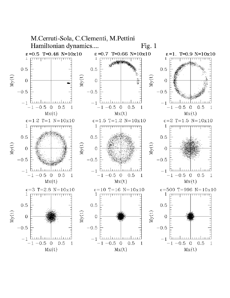
FIG. 1.: The magnetization vector ${\bf M}(t)$ computed along a trajectory for the $2d$ XY model at different temperatures on a lattice of $N=10\times 10$. Each point represents a vector ${\bf M}(t)$ at a certain time $t$.

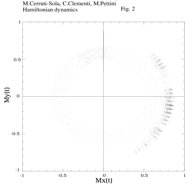
FIG. 2.: The magnetization vector ${\bf M}(t)$ at the temperature $T=0.74$, corresponding to the specific energy $\epsilon=0.8$ and computed in a time interval $\Delta t=10^{5}$, with a random initial configuration, on lattices of $N=10\times 10$ (external points) and of $N=200\times 200$ (internal points).

FIG. 3.: The magnetization vector ${\bf M}(t)$ at the temperature $T=1$, corresponding to the energy $\epsilon=1.2$, computed in a time interval $\Delta t=10^{5}$, with a random initial configuration on lattices of a) $N=10\times 10$, b) $N=50\times 50$, c) $N=100\times 100$ and d) $N=200\times 200$ sites, respectively.

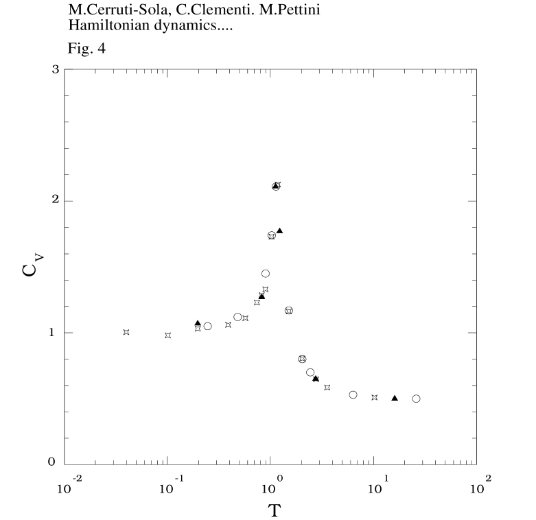
FIG. 4.: Specific heat at constant volume computed by means of Eq. (4) on a lattice of $N=10\times 10$ (open circles) and of $N=15\times 15$ (full triangles). Starlike squares refer to specific heat values computed by means of Eq. (3) on a lattice of $N=10\times 10$ .

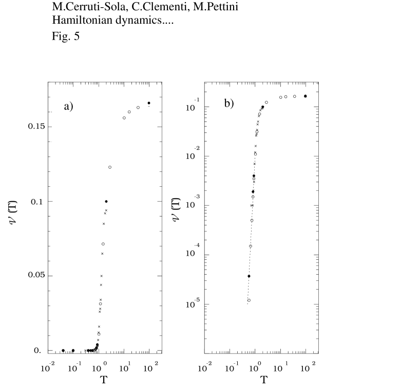
FIG. 5.: Vorticity function (plotted in a) linear scale and b) logarithmic scale) computed at different temperatures for lattices of $N=10\times 10$ (open circles) and $N=40\times 40$ (full circles). The results of the Monte Carlo simulations for a lattice of $N=60\times 60$ (crosses) are from [25]. The dashed line represents the power law ${\cal V}(t)\sim T^{10}$.

FIG. 6.: The largest Lyapunov exponents computed on different lattice sizes: $N=10\times 10$ (starred squares), $N=20\times 20$ (open triangles), $N=40\times 40$ (open stars), $N=50\times 50$ (open squares) and $N=100\times 100$ (open circles). In the inset, symbols have the same meaning.

FIG. 7.: The magnetization vector ${\bf M}(t)$, computed at the temperature $T=1.7$, on lattices of different sizes. By increasing the lattice dimensions, the longitudinal fluctuations decrease. The time interval $\Delta t=3.5\times 10^{4}-8\times 10^{4}$ is the same for the four simulations.

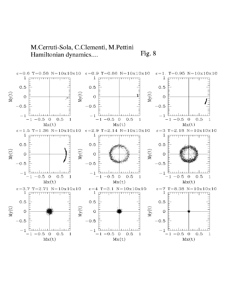
FIG. 8.: The magnetization vector ${\bf M}(t)$ computed at different temperatures on a lattice of $N=10\times 10\times 10$ spins.

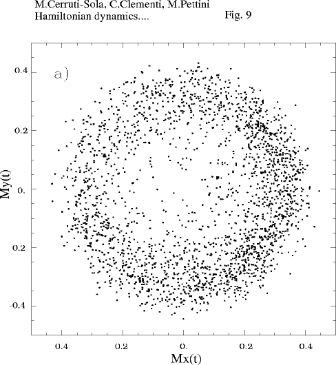
FIG. 9.: The magnetization vector ${\bf M}(t)$ computed at the temperature $T=2.22$ (slightly higher than the critical value) on lattices of a) $N=10\times 10\times 10$ and b)$N=15\times 15\times 15$, respectively. The time interval $\Delta t=0.5\times 10^{4}-1.5\times 10^{4}$ is the same for both simulations.

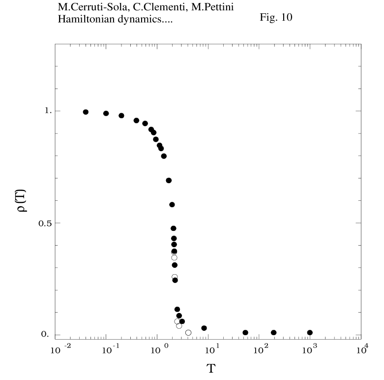
FIG. 10.: The dynamical order parameter, defined as the average of the modulus $|{\bf M}(t)|$ along a trajectory, computed on lattices of $N=10\times 10\times 10$ (full circles) and $N=15\times 15\times 15$ (open circles).

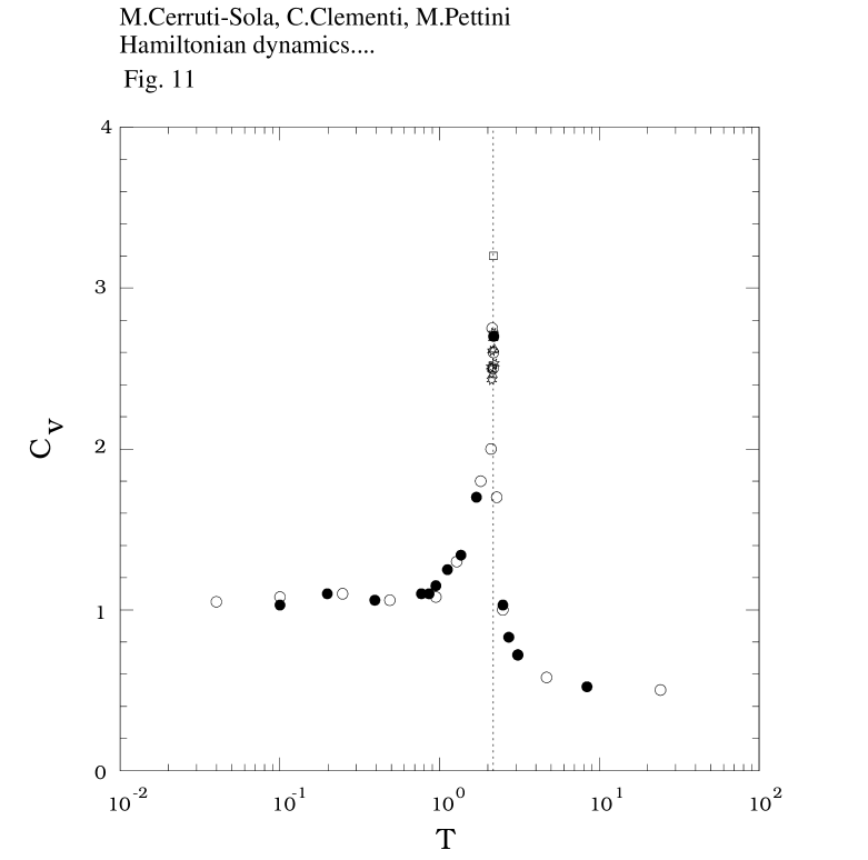
FIG. 11.: Specific heat at constant volume for the $3d$ model, computed by means of Eq. (4) on lattices of $N=8\times 8\times 8$ (open triangles), $N=10\times 10\times 10$ (open circles), $N=12\times 12\times 12$ (open stars) and $N=15\times 15\times 15$ (open squares) . Full circles refer to specific heat values computed by means of Eq. (3) on a lattice of $N=10\times 10\times 10$. The dashed line points out the critical temperature $T_{c}\simeq 2.17$ at which the phase transition occurs.

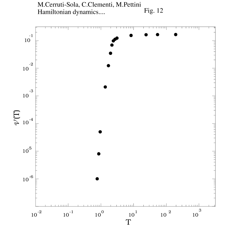
FIG. 12.: Vorticity function at different temperatures along a dynamical trajectory on a lattice of $N=10\times 10\times 10$ sites.

FIG. 13.: The largest Lyapunov exponents computed at different temperatures for the $3d$ model. Numerical results are for lattices of $N=10\times 10\times 10$ (open circles) and $N=15\times 15\times 15$ (open stars). In the inset, symbols have the same meaning. The dashed line points out the temperature $T_{c}\simeq 2.17$ of the phase transition. The solid line puts in evidence the departure of $\lambda_{1}(T)$ from the linear growth.

FIG. 14.: The largest Lyapunov exponents computed by means of the random dynamics algorithm (full circles) are plotted in comparison with those computed by means of the standard dynamics (open stars) for a lattice of $N=10\times 10\times 10$.

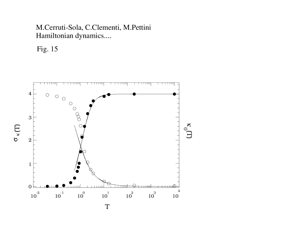
FIG. 15.: Time average of Ricci curvature (open circles) and its r.m.s. fluctuations (full circles) at different temperatures computed for a lattice of $N=40\times 40$ sites. Solid lines are the analytic estimates obtained from a high temperature expansion.

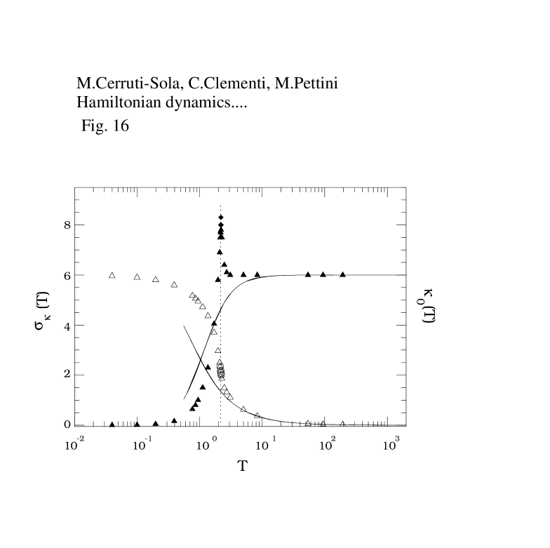
FIG. 16.: Time average of Ricci curvature (open triangles) and its r.m.s. fluctuations (full triangles) computed at different temperatures for a lattice of $N=10\times 10\times 10$. Open circles and full diamonds refer to a lattice size of $N=15\times 15\times 15$. Solid lines are the analytic estimates in the limit of high temperatures. The dashed line points out the temperature $T_{c}\simeq 2.17$ of the phase transition.

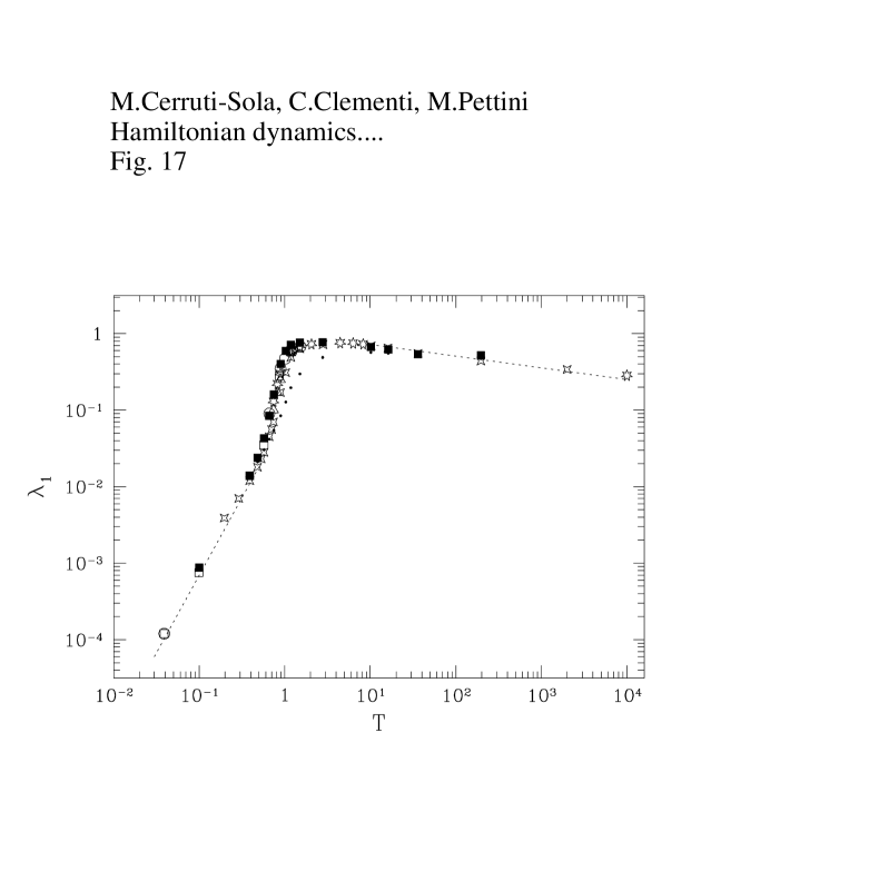
FIG. 17.: Analytic Lyapunov exponents computed for the $2d$ model by means of Eq.(14) without correction (dots) and incorporating the correction that accounts for the probability of obtaining negative sectional curvatures (full squares) for a lattice size of $N=40\times 40$ are plotted in comparison with the numerical values of Fig. 6. The dashed lines are the asymptotic behaviors at high and low temperatures in the thermodynamic limit.

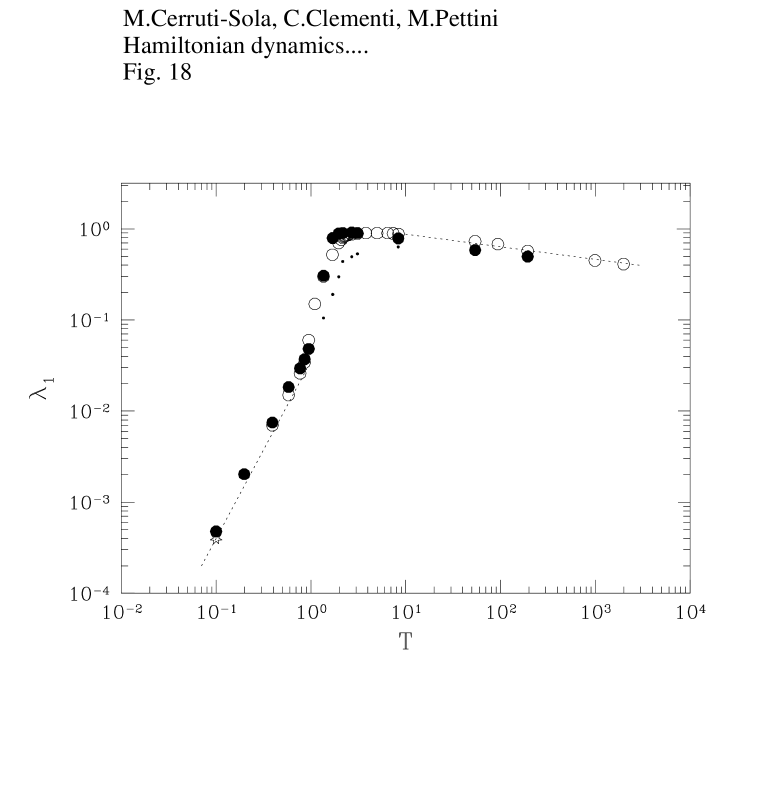
FIG. 18.: Analytic Lyapunov exponents computed for the $3d$ model by means of Eq.(14) without correction (dots) and incorporating the correction that accounts for the probability of obtaining negative sectional curvatures (full circles) are plotted in comparison with the numerical values of Fig. 13. The dashed lines are the asymptotic behaviors at high and low temperatures in the thermodynamic limit.

FIG. 19.: The deformation factor $D(E)=[\int_{\Sigma_{E}}(d\sigma/\|\nabla H\|)(M_{1}^{\star}/\|\nabla H\|)]\,/\,[\int_{\Sigma_{E}}d\sigma M_{1}]$ of Eq. (39) (open circles) is plotted vs. energy density $E/N$ and compared to the quantity $\langle 1/\|\nabla H\|^{2}\rangle$ (open triangles). $N=10\times 10\times 10$.

FIG. 20.: The normalized autocorrelation functions $\Gamma(\tau)$ are plotted vs. time $\tau$ for a lattice of $N=10\times 10\times 10$ and for four different values of the temperature (from top to bottom: $T=0.49,1.28,1.75,2.16$).

FIG. 21.: Autocorrelation times $\tau_{corr}$ are plotted vs. temperature $T$. The vertical dashed line points out the temperature $T_{c}\simeq 2.17$ at which the phase transition occurs.

REFERENCES

- [1] Electronic address: mcs@arcetri.astro.it
- [2] Electronic address: cclementi@ucsd.edu
- [3] Also at INFN, Sezione di Firenze, Italy. Electronic address: pettini@arcetri.astro.it
- [4] L. Caiani, L. Casetti, C. Clementi and M. Pettini, Phys. Rev. Lett. 79, 4361 (1997).
- [5] G. Gallavotti, Meccanica Statistica, (Quaderni C.N.R., Roma, 1995).
- [6] P. Hertel, and W. Thirring, Ann. Phys. (NY) 63, 520 (1971).
- [7] R.M. Lynden-Bell, in Gravitational Dynamics, O. Lahav, E. Terlevich and R.J. Terlevich, eds., Cambridge Contemporary Astrophysics, (Cambridge Univ. Press, 1996)
- [8] D.H.E. Gross, Phys. Rep. 279, 119 (1997); D.H.E. Gross and M.E. Madjet, Microcanonical vs. canonical thermodynamics, archived in cond-mat/9611192 see also the references quoted in these papers.
- [9] D.H.E. Gross, A. Ecker and X.Z. Zhang, Ann. Physik 5, 446 (1996).
- [10] A. Hüller, Z. Physik B95, 63 (1994); M. Promberger, M. Kostner, and A. Hüller, Magnetic properties of finite systems: microcanonical finite-size scaling, archived in cond-mat/9904265.
- [11] P. Butera and G. Caravati, Phys. Rev. A 36, 962 (1987).
- [12] X. Leoncini, A. Verga, and S. Ruffo, Phys. Rev. E 57, 6377 (1998).
- [13] A. Bonasera, V. Latora, A. Rapisarda, Phys. Rev. Lett. 75, 3434 (1995).
- [14] M. Antoni and S. Ruffo, Phys. Rev E 52, 2361 (1995).
- [15] M. Antoni and A. Torcini, Phys. Rev. E 57, R6233 (1998).
- [16] L. Caiani, L. Casetti and M. Pettini, J. Phys. A: Math. Gen., 31, 3357 (1998).
- [17] L. Caiani, L. Casetti, C. Clementi, G. Pettini, M. Pettini and R. Gatto, Phys. Rev E 57, 3886 (1998).
- [18] C. Clementi, Dynamics of homopolymeric chain models, Master Thesis, SISSA/ISAS, Trieste, (1996).
- [19] Ch. Dellago, H. A. Posch, W. G. Hoover, Phys. Rev. E 53, 1485 (1996); Ch. Dellago, H. A. Posch, Physica A 230, 364 (1996); Ch. Dellago and H. A. Posch, Physica A 237, 95 (1997); Ch. Dellago and H. A. Posch, Physica A 240, 68 (1997) .
- [20] V. Mehra, R. Ramaswamy, preprint chao-dyn/9706011.
- [21] S. K. Nayak, P. Iena, K. D. Ball and R. S. Berry, J. Chem. Phys. 108, 234 (1998).
- [22] M.-C. Firpo, Phys. Rev. E 57, 6599 (1998).
- [23] V. Latora, A. Rapisarda, and S. Ruffo, Phys. Rev. Lett. 80, 692 (1998).
- [24] V. Latora, A. Rapisarda, and S. Ruffo, Physica D (1998), in press.
- [25] J. Tobochnik, and G. V. Chester, Phys. Rev. B20, 3761 (1979).
- [26] R. Gupta, and C.F. Baillie, Phys. Rev. B45, 2883 (1992).
- [27] L. Casetti, Phys. Scr. 51, 29 (1995).
- [28] E. M. Pearson, T. Halicioglu, and W. A. Tiller, Phys. Rev. A32, 3030 (1985).
- [29] A thorough discussion about ergodicity breaking, non interchangeability of and limits can be found in: R.G. Palmer, Adv. Phys. 31, 669 (1982).
- [30] J. Lebowitz, J. Percus, and L. Verlet, Phys. Rev. 153, 250 (1967).
- [31] L. Casetti, C. Clementi and M. Pettini, Phys. Rev. E 54, 5969 (1996).
- [32] M.Pettini, Phys. Rev. E 47, 828 (1993).
- [33] L. P. Eisenhart, Ann. of Math. 30, 591 (1939).
- [34] M. P. Do Carmo, Riemannian Geometry (Birkhäuser, Boston, 1992).
- [35] M.Cerruti-Sola and M. Pettini, Phys. Rev. E53, 179 (1996); M.Cerruti-Sola, R. Franzosi and M. Pettini, Phys. Rev. E56, 4872 (1997).
- [36] L. Casetti, E.G.D. Cohen, and M. Pettini, Phys. Rev. Lett. 82, 4160 (1999).
- [37] R. Franzosi, L. Casetti, L. Spinelli, and M. Pettini, Phys. Rev. E60, 5009 (1999).
- [38] R. Franzosi, M. Pettini, and L. Spinelli, Topology and Phase transitions: a paradigmatic evidence, Phys. Rev. Lett., (1999) submitted; archived in cond-mat/9911235.
- [39] J.A. Thorpe, Elementary Topics in Differential Geometry, (Springer, New York, 1979).
- [40] P. Laurence, Zeit. Angew. Math. Phys.40, 258 (1989).
- [41] A similar formula is obtained in: H.H. Rugh, J.Phys.A: Math. Gen. 31, 7761 (1998), though without using the result of Ref. [40], and in: C. Giardinà, R. Livi, J. Stat. Phys. 98, 1027 (1998); however in these papers the relation between temperature and mean curvature was not established.
- [42] S. Chern, and R.K. Lashof, Michigan Math. J. 5, 5 (1958).
- [43] M. Nakahara, Geometry, Topology and Physics, (Adam Hilger, Bristol, 1989).
- [44] The mathematical details to justify such an assumption are discussed in: R. Franzosi, Geometrical and Topological Aspects in the study of Phase Transitions, PhD thesis, Department of Physics, University of Florence, (1999).
- [45] D.H.E. Gross and E. Votyakov, Phase transitions in finite systems = topological peculiarities of the microcanonical entropy surface, archived in cond-mat/9904073; D.H.E. Gross and E. Votyakov, Phase transitions in “small” systems, archived in cond-mat/9911257; D.H.E. Gross, Phase Transitions without thermodynamic limit, archived in cond-mat/9805391.
- [46] E. Gozzi and M. Reuter, Phys. Lett. B 233, 383 (1989).
- [47] E. Gozzi, M. Reuter and W. D. Thacker, Chaos, Solitons & Fractals 2, 441 (1992).
- [48] E. Gozzi and M. Reuter, Chaos, Solitons & Fractals 4, 1117 (1994).
- [49] M. Creutz, Phys. Rev. Lett. 50, 1411 (1983).