Extremal-point Densities of Interface Fluctuations

Abstract

We introduce and investigate the stochastic dynamics of the density of local extrema (minima and maxima) of non-equilibrium surface fluctuations. We give a number of exact, analytic results for interface fluctuations described by linear Langevin equations, and for on-lattice, solid-on-solid surface growth models. We show that in spite of the non-universal character of the quantities studied, their behavior against the variation of the microscopic length scales can present generic features, characteristic to the macroscopic observables of the system. The quantities investigated here present us with tools that give an entirely un-orthodox approach to the dynamics of surface morphologies: a statistical analysis from the short wavelength end of the Fourier decomposition spectrum. In addition to surface growth applications, our results can be used to solve the asymptotic scalability problem of massively parallel algorithms for discrete event simulations, which are extensively used in Monte-Carlo type simulations on parallel architectures.

I Introduction and Motivation

The aim of statistical mechanics is to relate the macroscopic observables to the microscopic properties of the system. Before attempting any such derivation one always has to specify the spectrum of length-scales the analysis will comprise: while ‘macroscopic’ is usually defined in a unique way by the every-day-life length scale, the ‘microscopic’ is never so obvious, and the choice of the best lower-end scale is highly non-universal, it is system dependent, usually left to our physical ‘intuition’, or it is set by the limitations of the experimental instrumentation. It is obvious that in order to derive the laws of the gaseous matter we do not need to employ the physics of elementary particles, it is enough to start from an effective microscopic model (or Hamiltonian) on the level of molecular interactions. Then starting from the equations of motion on the microscopic level and using a statistic and probabilistic approach, the macroscale physics is derived. In this ‘long wavelength’ approach most of the microscopic, or short wavelength information is usually redundant and it is scaled away.

Sometimes however, microscopic quantities are important and directly contribute to macroscopic observables, e.g., the nearest-neighbor correlations in driven systems determine the current, in model B the mobility, in kinetic Ising model the domain-wall velocity, in parallel computation the utilization (efficiency) of conservative parallel algorithms, etc. Once a lower length scale is set on which we can define an effective microscopic dynamics, it becomes meaningful to ask questions about local properties at this length scale, e.g. nearest neighbor correlations, contour distributions, extremal-point densities, etc. These quantities are obviously not universal, however their behavior against the variation of the length scales can present qualitative and universal features. Here we study the dynamics of macroscopically rough surfaces via investigating an intriguing miscroscopic quantity: the density of extrema (minima) and its finite size effects. We derive a number of analytical results about these quantities for a large class of non-equilibrium surface fluctuations described by linear Langevin equations, and solid-on-solid (SOS) lattice-growth models. Besides their obvious relevance to surface physics our technique can be used to show [1] the asymptotic scalability of conservative massively parallel algorithms for discrete-event simulation, i.e., the fact that the efficiency of such computational schemes does not vanish with increasing the number of processing elements, but it has a lower non-trivial bound. The solution of this problem is not only of practical importance from the point of view of parallel computing, but it has important consequences for our understanding of systems with asynchronous parallel dynamics, in general. There are numerous dynamical systems both man-made, and found in the nature, that contain a “substantial amount” of parallelism. For example,

1) in wireless cellular communications the call arrivals and departures are happening in continuos time (Poisson arrivals), and the discrete events (call arrivals) are not synchronized by a global clock. Nevertheless, calls initiated in cells substantially far from each other can be processed simultaneously by the parallel simulator without changing the poissonian nature of the underlying process. The problem of designing efficient dynamic channel allocation schemes for wireless networks is a very difficult one and currently it is done by modelling the network as a system of interacting continuous time stochastic automata on parallel architectures [2].

2) in magnetic systems the discrete events are the spin flip attempts (e.g., Glauber dynamics for Ising systems). While traditional single spin flip dynamics may seem inherently serial, systems with short range interactions can be simulated in parallel: spins far from each other with different local simulated times can be updated simultaneously. Fast and efficient parallel Monte-Carlo algorithms are extremely welcome when studying metastable decay and hysteresis of kinetic Ising ferromagnets below their critical temperature, see [3] and references therein.

3) financial markets, and especially the stock market is an extremely dynamic, high connectivity network of relations, thousands of trades are being made asynchronously every minute.

4) the brain. The human brain, in spite of its low weight of approx. 1kg, and volume of 1400 $cm^{3}$, it contains about 100 billion neurons, each neuron being connected through synapses to approximately 10,000 other neurons. The total number of synapses in a human brain is about 1000 trillion ($10^{15}$). The neurons of a single human brain placed end-to-end would make a “string” of an enourmous lenght: 250,000 miles [4]. Assuming that each neuron of a single human cortex can be in two states only (resting or acting), the total number of different brain configurations would be ${2^{10}}^{11}$. According to Carl Sagan, this number is greater than the total number of protons and electrons of the known universe, [4]. The brain does an incredible amount of parallel computation: it simultaneously manages all of our body functions, we can talk and walk at the same time, etc.

5) evolution of networks such as the internet, has parallel dynamics: the local network connectivity changes concurrently as many sites are attached or removed in different locations. As a matter of fact the physics of such dynamic networks is a currently heavily investigated and a rapidly emerging field [5].

In order to present the basic ideas and notions in the simplest way, in the following we will restrict ourselves to one dimensional interfaces that have no overhangs. The restriction on the overhangs may actually be lifted with a proper parametrization of the surface, a problem to which we will return briefly in the concluding section. The first visual impression when we look at a rough surface $h(x,t)$ is the extent of the fluctuations perpendicular to the substrate, in other words, the width of the fluctuations. The width (or the rms of the height $h$ of the fluctuations) is probably the most extensively studied quantity in interface physics, due to the fact that its definition is simply quantifiable and therefore measurable:

$$w(L,t)=\sqrt{\;\overline{\left[h(x,t)\right]^{2}}-\left[\overline{h(x,t)}\right]^{2}}\;,$$ (1)

where the overline denotes the average over the substrate. It is well-known that this quantity characterizes the long wavelength behavior of the fluctuations, the high frequency components being averaged out in (1). The short wavelength end of the spectrum has been ignored in the literature mainly because of its non-universal character, and also because it seemed to lack such a simple quantifiable definition as the width $w$.

In the following we will present a quantity that is almost as simple and intuitive as the width $w$ but it characterizes the high frequency components of the fluctuations and it is simply quantifiable. For illustrative purposes let us consider the classic Weierstrass function defined as the $M\to\infty$ limit of the smooth functions $W_{M}(a,b;x)$:

$$W(a,b;x)=\lim_{M\to\infty}W_{M}(a,b;x)=\lim_{M\to\infty}\sum_{m=0}^{M}a^{-m}\cos\left(b^{m}x\right)\;,\;\;\;a,b>1$$ (2)

Figure 1a shows the graph of $W_{M}$ at $a=2$ and $b=3$ (arbitrary values) for $M=0,1,2,3,4$ in the interval $x\in[0,4\pi]$. As one can see, by increasing $M$ we are adding more and more detail to the graph of the function on finer and finer length-scales. Thus $M$ plays the role of a regulator for the microscopic cut-off length which is $b^{-M}$, and for $M=\infty$ and $b>a$, the function becomes nowhere differentiable as it was shown by Hardy [6].

Comparing the graphs of $W_{M}$ for lower $M$ values with those for higher $M$-s we observe that the width effectively does not change, however the curves look qualitatively very different. This is obvious from (2): adding an extra term will not change the long wavelength modes, but adds a higher frequency component to the Fourier spectrum of the graph. We need to operationally define a quantifiable parameter which makes a distinction between a much ‘fuzzier’ graph, such as $M=4$ and a smoother one, such as $M=1$. The natural choice based on Figure 1a is the number of local minima (or extrema) in the graph of function. In Figure 1b we present the number of local minima $u_{M}$ vs. $M$ for two different values of $b$, $b=2.8$ and $b=1.8$, while keeping $a$ at the same value of $a=2$. For all $b$ values (not only for these two) the leading behaviour is exponential: $u_{M}\sim\lambda^{M}$. The inset in Figure 1b shows the dependence of the rate $\lambda$ as a function of $b$ for fixed $a$. We observe that for $b>a$, $\lambda=b$, but below $b=a$ the dependence crosses over to another, seemingly linear function. For $b>a$ the amplitude of the extra added term in $W_{M+1}$ is large enough to prevent the cancellation of the newly appearing minima by the drop in the local slope of $W_{M}$. At $b\leq a$ the number of cancelled extrema starts to increase drastically with an exponential trend, leading to the crossover seen in the inset of Figure 2b. It has been shown that the fractal dimension of the Weierstrass function for $b>a$ is given by $D_{0}=\ln{b}/\ln{a}$ [7], [8]. For $b\leq a$ the Weierstrass curve becomes non-fractal with a dimension of $D_{0}=1$. By varying $b$ with respect to $a$, we are crossing a fractal-smooth transition at $b=a$. The very intriguing observation we just come across is that even though we are in the smooth regime ($b<a$) the density of minima is still a diverging quantity (the $b=1.8$ curve in Figure 1b). It is thus possible to have an infinite number of ‘wrinkles’ in the Weierstrass function without having a diverging length, without having a fractal in the classical sense. The transition from fractal to smooth, as $b$ is lowered appears as a non-analyticity in the divergence rate of the curve’s wrinkledness. A rigorous analytic treatment of this problem seems to be highly non-trivial and we propose it as an open question to the interested reader.

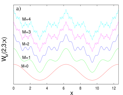
FIG. 1.: a) the function $W_{M}(a,b;x)$ at $a=2$, $b=3$ and $M=0,1,2,3,4$. b) The scaling $u_{M}\sim\lambda^{M}$ of the number of local minima for $b=2.8$ (plusses) and $b=1.8$ (crosses). The inset shows $\lambda$ vs. $b$ while keeping $a$ constant, $a=2$.

The simple example shown above suggests that there is novel and non-trivial physics lying behind the analysis of extremal point densities, and it gives extra information on the morphology of interfaces. Given an interface $h(x,t)$, we propose a quantitative form that characterizes the density of minima via a ‘partition-function’ like expression, which is hardly more complex than Eq. (1) and gives an alternate description of the surface morphology:

$$u_{q}(L,[h])=\frac{1}{L}\sum_{i}\left[K(x_{i})\right]^{q}\;,\;\;\;q>0\;,\;\;\;\mbox{$x_{i}$ are non-degenerate minima of $h$}$$ (3)

with $K(x_{i})$ denoting the curvature of $h$ at the local (non-degenerate) minimum point $x_{i}$. The variable $q$ can be conceived as ‘inverse temperature’. Obviously, for $q=0$ we obtain the number of local minima per unit interface length. The rigorous mathematical description and definitions lying at the basis of (3) is being presented in Section IV. The quantity in Eq. (3) is reminiscent to the partition function used in the definition of the thermodynamical formalism of one dimensional chaotic maps [9] and also to the definition of the dynamical or Rényi entropies of these chaotic maps. In that case, however the curvatures at the minima are replaced by cylinder intervals and/or the visiting probabilities of these cylinders.

We present a detailed analysis for the above quantity in case of a large class of linear Langevin equations of type $\partial h/\partial t=-\nu(-\nabla^{2}h)^{z/2}+\eta(x,t)$, where $\eta$ is a Gaussian noise term, and $z$ a positive real number. These Langevin equations are found to describe faithfully the fluctuations of monoatomic steps on various substrates, see for a review Ref. [13]. One of the interesting conclusions we came to by studying the extremal-point densities on such equations is that depending on the value of $z$ the typical surface morphology can be fractal, or locally smooth, and the two regimes are separated by a critical $z$ value, $z_{c}$. In the fractal case, the interface will have infinitely many minima and cusps just as in the case of the nondifferentiable Weierstrass function (2), and the extremal point densities become infinite, or if the problem is discretized onto a lattice with spacing $a$, a power-law diverging behavior is observed as $a\to 0^{+}$ for these densities. This sudden change of the ‘intrinsic roughness’ may be conceived as a phase transition even in an experimental situation. Changing a parameter, such as the temperature, the law describing the fluctuations can change since the mechanism responsible for the fluctuations can change character as the temperature varies. For example, it has been recently shown using Scanning Tunneling Microscope (STM) measurements [10], that the fluctuations of single atom layer steps on $Cu$ (111) below $T=300\mbox{ }^{o}C$ correspond to the perifery diffusion mechanism ($z=4$), but above this temperature (such as $T=500\mbox{ }^{o}C$ in their measurements) the mechanism is attachement-detachment where $z=2$, see also Ref. [11, 12].

The paper is organized as follows: In Sections II and III we define and investigate on several well known on-lattice models the minimum point density and derive exact results in the steady-state ($t\to\infty$) including finite size effects. As a practical application of these on-lattice results, we briefly present in Subsection III.B a lattice surface-growth model which exactly describes the evolution of the simulated time-horizon for conservative massively parallel schemes in parallel computation, and solve a long-standing asymptotic scalability question for these update schemes. In Section IV we lay down a more rigorous mathematical treatment for extremal point densities, and stochastic extremal point densities on the continuum, with a detailed derivation for a large class of linear Langevin equations (which are in fact the continuum counterparts of the discrete ones from Section II). The more rigorous treatment allows for an exact analytical evaluation not only in the steady-state, but for all times! We identify novel characteristic dimensions that separate regimes with divergent extremal point densities from convergent ones and which give a novel understanding of the short wavelength physics behind these kinetic roughening processes.

II Linear surface growth models on the lattice

In the present Section we focus on discrete, one dimensional models from the linear theory of kinetic roughening [14, 18]. Let us consider a one dimensional substrate consisting of $L$ lattice sites, with periodic boundary conditions. For simplicity the lattice constant is taken as unity, which clearly, represents the lower cut-off length for the effective equation of motion. For the moment let us study the discretized counterpart of the general Langevin equation that describes the linear theory of Molecular Beam Epitaxy (MBE) [15, 16]:

$$\partial_{t}h_{i}(t)=\nu\nabla^{2}h_{i}(t)-\kappa\nabla^{4}h_{i}(t)+\eta_{i}(t)\;,$$ (4)

where $\eta_{i}(t)$ is Gaussian white noise with

$$\langle\eta_{i}(t)\eta_{i}(t^{\prime})\rangle=2D\;\delta_{i,j}\;\delta(t-t^{\prime})\;,$$ (5)

and $\nabla^{2}$ is the discrete Laplacian operator, i.e., $\nabla^{2}f_{j}=f_{j+1}+f_{j-1}-2f_{j}$, applied to an arbitrary lattice function $f_{j}$. This equation arrises in MBE with both surface diffusion mechanism (the 4th order, or curvature term) and desorption mechanism (the 2nd order, or diffusive term) present and it has been studied extensively by several authors [15, 17]. Stability requires $\nu\geq 0$ and $\kappa\geq 0$ (as a matter of fact, on the lattice is enough to have $\nu>0$ and $\kappa\geq-\nu/2$). Starting from a completely flat initial condition, the interface roughens until the correlation length $\xi$ reaches the size of the system $\xi\simeq L$, when the roughening saturates over into a steady-state regime. The process of kinetic roughening is controlled by the intrinsic length scale [17], $\sqrt{\kappa/\nu}$. Below this lengthscale the roughening is dominated by the surface diffusion or Mullins [19] term (the 4th order operator) but above it is characterized by the evaporation piece (the diffusion) or Edwards-Wilkinson [20] term. Since eq. (4) is translationaly invariant and linear in $h$ it can be solved via the discrete Fourier-transform:

$$\tilde{h}_{k}=\sum_{j=0}^{L-1}e^{-ikj}h_{i}\;,\;\;k=\frac{2\pi n}{L}\;,\;\;n=0,1,2,\ldots,L-1\;.$$ (6)

Then eq. (4) translates into

$$\partial_{t}\tilde{h}_{k}(t)=-\left[2\nu(1-\cos(k))+4\kappa(1-\cos(k))^{2}\right]\tilde{h}_{k}(t)+\tilde{\eta}_{k}(t)\;,$$ (7)

with

$$\langle\tilde{\eta}_{k}(t)\tilde{\eta}_{k^{\prime}}(t^{\prime})\rangle=2DL\;\delta_{(k+k^{\prime})\;\mbox{mod}\;2\pi,0}\;\delta(t-t^{\prime})$$ (8)

Following the definition of the equal-time structure factor for $S(k,t)$, namely

$$S^{h}(k,t)L\delta_{(k+k^{\prime})\;\mbox{mod}\;2\pi,0}\equiv\langle\tilde{h}_{k}(t)\tilde{h}_{k^{\prime}}(t)\rangle\;,$$ (9)

one obtains for an initially flat interface:

$$S^{h}(k,t)=S^{h}(k)\left(1-e^{-(4\nu(1-\cos(k))+8\kappa(1-\cos(k))^{2})t}\right)\;.$$ (10)

In the above equation

$$S^{h}(k)\equiv\lim_{t\rightarrow\infty}S^{h}(k,t)=\frac{D}{2\nu(1-\cos(k))+4\kappa(1-\cos(k))^{2}}$$ (11)

is the steady-state structure factor.

For $\nu\neq 0$, and in the asymptotic scaling limit where $L\gg\sqrt{\kappa/\nu}$, the model belongs to the EW universality class and the roughening exponent is $\alpha=1/2$ (it is defined through the scaling $L^{2\alpha}$ of the interface width $\langle w_{L}^{2}(t)\rangle=(1/L)\langle\sum_{i=1}^{L}[h_{i}(t)-\overline{h}]^{2}\rangle$ in the steady state). The presence of the curvature term does not change the universal scaling properties for the surface width, and one finds the same exponents as for the pure EW ($\kappa=0$) case in eq. (4). For $\nu=0$ the surface is purely curvature driven ($z=4$) and the model belongs to a different universality class where the steady-state width scales with a roughness exponent of $\alpha=3/2$.

In the following we will be mostly interested in some local steady-state properties of the surface ${h_{i}}$. In particular, we want to find the density of local minima for the surface described by (4). The operator which measures this quantity is

$$u=\frac{1}{L}\sum_{i=1}^{L}\Theta(h_{i-1}-h_{i})\Theta(h_{i+1}-h_{i})\;.$$ (12)

This expression motivates the introduction of the local slopes, $\phi_{i}=h_{i+1}-h_{i}$. In this representation the operator for the density of local minima (for the original surface) is

$$u=\frac{1}{L}\sum_{i=1}^{L}\Theta(-\phi_{i-1})\Theta(\phi_{i})\;,$$ (13)

and its steady-state average is $\langle u\rangle=\langle\Theta(-\phi_{i-1})\Theta(\phi_{i})\rangle=\langle\Theta(-\phi_{1})\Theta(\phi_{2})\rangle$, due to translational invariance. The average density of local minima is the same as the probability that at a randomly chosen site of the lattice the surface exhibits a local minimum. It is governed by the nearest-neighbor two-slope distribution, which is also Gaussian and fully determined by $\langle\phi_{1}^{2}\rangle=\langle\phi_{2}^{2}\rangle$ and $\langle\phi_{1}\phi_{2}\rangle$:

$$P^{nn}(\phi_{1},\phi_{2})\propto e^{-\frac{1}{2}\phi_{j}A^{\rm nn}_{jk}\phi_{k}}\;,\;\;\;j,k=1,2\;,$$ (14)

where

$$A^{\rm nn}=\left(\begin{array}[]{cc}\langle\phi_{1}^{2}\rangle&\langle\phi_{1}\phi_{2}\rangle\\ \langle\phi_{1}\phi_{2}\rangle&\langle\phi_{1}^{2}\rangle\end{array}\right)^{-1}$$ (15)

As we derive in Appendix A, the density of local minima only depends on the ratio $\langle\phi_{1}\phi_{2}\rangle/\langle\phi_{1}^{2}\rangle$:

$$\langle u\rangle=\frac{1}{2\pi}\arccos\left(\frac{\langle\phi_{1}\phi_{2}\rangle}{\langle\phi_{1}^{2}\rangle}\right)\;.$$ (16)

Finite-size effects of $\langle u\rangle$ are obviously carried through those of the correlations. First we find the steady-state structure factor for the slopes. Since $\tilde{\phi}_{k}=(1-e^{-ik})\tilde{h}_{k}$, we have $S^{\phi}(k)=2(1-\cos(k))S^{h}(k)$. Then from (11) one obtains:

$$S^{\phi}(k)=\frac{D}{\nu+2\kappa(1-\cos(k))}\;,\;\;\mbox{for}\;\;k\neq 0\;,\;\;\;\mbox{and}\;\;\;S^{\phi}(k)=0\;,\;\;\mbox{for}\;\;k=0\;.$$ (17)

The former automatically follows from the $\sum_{i=1}^{L}\phi_{i}=0$ relation. Then we obtain the slope-slope correlations

$$C^{\phi}_{L}(l)\equiv\langle\phi_{i}\phi_{i+l}\rangle=\frac{1}{L}\sum_{n=1}^{L-1}e^{i\frac{2\pi n}{L}l}S^{\phi}\left(\frac{2\pi n}{L}\right)\;.$$ (18)

With the help of Poisson summation formulas, in Appendix B we show a derivation for the exact spatial correlation function, which yields

$$C^{\phi}_{L}(l)=\frac{D}{\nu+2\kappa}\left\{\frac{b^{|l|}}{\sqrt{1-a^{2}}}-\frac{1}{1-a}\frac{1}{L}+\frac{b^{L}}{1-b^{L}}\frac{b^{l}+b^{-l}}{\sqrt{1-a^{2}}}\right\}\;,\;\;\;|l|\leq L\;,$$ (19)

with

$$a\equiv\frac{2\kappa}{\nu+2\kappa}\;,\;\;\;\mbox{and}\;\;\;b\equiv\frac{1-\sqrt{1-a^{2}}}{a}\;.$$ (20)

We have $|a|\leq 1$ and $b\leq 1$. The second term in the bracket in (19) gives a uniform power law correction, while the third one gives an exponential correction to the correlation function in the thermodynamic limit. For $\nu\neq 0$ and $L\rightarrow\infty$ one obtains

$$C^{\phi}_{\infty}(l)=\frac{D}{\nu+2\kappa}\frac{b^{|l|}}{\sqrt{1-a^{2}}}=\frac{D}{\nu+2\kappa}\frac{e^{-|l|/\xi^{\phi}_{\infty}}}{\sqrt{1-a^{2}}}$$ (21)

where we define the correlation length of the slopes for an infinite system as:

$$\xi^{\phi}_{\infty}\equiv-\frac{1}{\ln(b)}\;.$$ (22)

In the $\nu\rightarrow 0$ limit it becomes the intrinsic correlation length which diverges as $\nu^{-1/2}$: $\xi^{\phi}_{\infty}\stackrel{{\scriptstyle\nu\rightarrow 0}}{{\simeq}}\sqrt{\kappa/\nu}$ and

$$C^{\phi}_{\infty}(l)\stackrel{{\scriptstyle\nu\rightarrow 0}}{{\simeq}}\frac{D}{2\kappa}\left(\sqrt{\frac{\kappa}{\nu}}-|l|\right)\simeq\frac{D}{2\kappa}\left(\xi^{\phi}_{\infty}-|l|\right)\;.$$ (23)

In this limit the slopes (separated by any finite distance) become highly correlated, and one may start to anticipate that the density of local minima will vanish for the original surface $\{h_{i}\}$. In the following two subsections we investigate the density of local minima and its finite-size effects for the Edwards-Wilkinson and the Mullins cases.

A Density of local minima for Edwards-Wilkinson term dominated regime

To study the finite size effects for the local minimum density, we neglect the exponentially small correction in (19), so in the asymptotic limit, where $L\gg\xi^{\phi}_{\infty}$, $C^{\phi}_{L}(l)$ decays exponentially with uniform finite-size corrections:

$$C^{\phi}_{L}(l)\simeq\frac{D}{\nu+2\kappa}\left\{\frac{b^{|l|}}{\sqrt{1-a^{2}}}-\frac{1}{1-a}\frac{1}{L}\right\}\;$$ (24)

This holds for the special case $\kappa=0$ as well, (in fact, there the exponential correction exatly vanishes) leaving

$$C^{\phi}_{L}(l)=\frac{D}{\nu}\left(\delta_{l,0}-\frac{1}{L}\right)\;.$$ (25)

Now, emplying eq. (16), we can obtain the density of minima as:

$$\langle u\rangle_{L}=\frac{1}{2\pi}\arccos\left(\frac{C^{\phi}_{L}(1)}{C^{\phi}_{L}(0)}\right)\simeq\frac{1}{2\pi}\arccos(b)+\frac{1}{2\pi}\sqrt{\frac{1-b}{1+b}}\sqrt{\frac{1+a}{1-a}}\frac{1}{L}\;,$$ (26)

Again, for the $\kappa=0$ case one has a compact exact expression and the corresponding large $L$ behavior:

$$\langle u\rangle_{L}=\frac{1}{2\pi}\arccos\left(-\frac{1}{L-1}\right)\simeq\frac{1}{4}+\frac{1}{2\pi}\frac{1}{L}\;,$$ (27)

which can also be obtained by taking the $\kappa\rightarrow 0$ limit in (26). To summarize, as long as $\nu\neq 0$, the model belongs to the EW universality class, and in the steady state, the density of local minima behaves as

$$\langle u\rangle_{L}\simeq\langle u\rangle_{\infty}+\frac{\rm const.}{L}\;,$$ (28)

where $\langle u\rangle_{\infty}$ is the value of the density of local minima in the thermodynamic limit:

$$\langle u\rangle_{\infty}=\frac{1}{2\pi}\arccos(b)\;.$$ (29)

Note that this quantity can be small, but does not vanish if $\nu$ is close but not equal to $0$. Further, the system exhibits the scaling (28) for asymptotically large systems, where $L\gg\xi^{\phi}_{\infty}$. It is important to see in detail how $\langle u\rangle_{\infty}$ behaves as $\nu\rightarrow 0$:

$$\langle u\rangle_{\infty}\stackrel{{\scriptstyle\nu\rightarrow 0}}{{\simeq}}\frac{1}{2\pi}\arccos\left(1-\sqrt{2}\sqrt{1-a}\right)\simeq\frac{1}{2\pi}\arccos\left(1-\sqrt{\frac{\nu}{\kappa}}\right)\simeq\frac{1}{2\pi}\left(2\sqrt{\frac{\nu}{\kappa}}\right)^{1/2}\simeq\frac{\sqrt{2}}{2\pi}\frac{1}{\sqrt{\xi^{\phi}_{\infty}}}\;.$$ (30)

Thus, the density of local minima for an infinite system vanishes as we approach the purely curvature driven ($\nu\rightarrow 0$) limit. Simply speaking, the local slopes become “infinitely” correlated, such that $C^{\phi}_{\infty}(l)$ diverges [according to eq. (23)], and the ratio $C^{\phi}_{\infty}(l)/C^{\phi}_{\infty}(0)$ for any fixed $l$ tends to $1$. This is the physical picture behind the vanishing density of local minima.

B Density of local minima for the Mullins term dominated regime

Here we take the $\nu\rightarrow 0$ limit first and then study the finite size effects in the purely curvature driven model. The slope correlations are finite for finite $L$ as can be seen from eq. (18), since the $n=0$ term is not included in the sum! Thus, in the exact closed formula (19) a careful limiting procedure has to be taken which indeed yields the internal cancellation of the apparently divergent terms. Then one obtains the exact slope correlations for the $\nu=0$ case:

$$C^{\phi}_{L}(l)=\frac{D}{2\kappa}\left\{\frac{L}{6}\left(1-\frac{1}{L^{2}}\right)-|l|\left(1-\frac{|l|}{L}\right)\right\}\;$$ (31)

and for the local minimum density:

$$\langle u\rangle_{L}=\frac{1}{2\pi}\arccos\left(1-\frac{6}{L+1}\right)\simeq\frac{\sqrt{3}}{\pi}\frac{1}{\sqrt{L}}$$ (32)

It vanishes in the thermodynamic limit, and hence, one observes that the limits $\nu\rightarrow 0$ and $L\rightarrow\infty$ are interchangable. For $\nu=0$, $L$ is directly associated with the correlation length and we can define $\xi^{\phi}_{L}\equiv L/6$. Then the correlations and the density of local minima takes the same scaling form as eqs. (23) and (30):

$$C^{\phi}_{L}(l)\simeq\frac{D}{2\kappa}\left(\xi^{\phi}_{L}-|l|\right)\;,$$ (33)

and

$$\langle u\rangle_{L}\simeq\frac{\sqrt{2}}{2\pi}\frac{1}{\sqrt{\xi^{\phi}_{L}}}\;.$$ (34)

C Scaling considerations for higher order equations

Let us now consider another equation but with a generalized relaxational term that includes the Edwards Wilkinson and the noisy Mullins equation as particluar cases:

$$\partial_{t}h_{i}(t)=-\nu\left(-\nabla^{2}\right)^{z/2}h+\eta_{i}(t)\;.$$ (35)

where $z$ is a positive real number (not necessarily integer). Other $z$ values of experimental interest are $z=1$, relaxation through plastic flow, [19, 18]), and $z=3$ terrace-diffusion mechanism [11, 12, 13]. For early times, such that $t\ll L^{z}$, the interface width $\langle w_{L}^{2}(t)\rangle$ increases with time as

$$\langle w_{L}^{2}(t)\rangle\sim t^{2\beta}\;,$$ (36)

where $\beta=(z-1)/2z$ [14, 18]. In the $t\rightarrow\infty$ limit, where $t\gg L^{z}$, the interface width saturates for a finite system, but diverges with $L$ according to $\langle w_{L}^{2}(\infty)\rangle\sim L^{2\alpha}$ where $\alpha=(z-1)/2$ is the roughness exponent [14, 18].

For $z=4$ (curvature driven interface) we saw that the slope fluctuation behaves as $C^{\phi}_{L}(0)=\langle\phi_{i}^{2}\rangle\sim L$. For higher $z$ for the slope-slope correlation function one can deduce

$$C^{\phi}_{L}(l)=\frac{D}{L}\sum_{n=1}^{L-1}\frac{e^{i\frac{2\pi n}{L}l}}{\nu\left[2\left(1-\cos\left(\frac{2\pi n}{L}\right)\right)\right]^{\frac{z-2}{2}}}\;.$$ (37)

It is divergent in the $L\rightarrow\infty$ limit, as a result of infinitely small wave-vectors $\sim 1/L$, and we can see that

$$C^{\phi}_{L}(0)\sim L^{z-3}\;.$$ (38)

It is also useful to define the slope difference correlation function

$$G^{\phi}_{L}(l)\equiv\langle(\phi_{i+l}-\phi_{i})^{2}\rangle$$ (39)

for which one can write

$$G^{\phi}_{L}(l)=\frac{D}{L}\sum_{n=1}^{L-1}\frac{2\left(1-\cos\left(\frac{2\pi n}{L}l\right)\right)}{\nu\left[2\left(1-\cos\left(\frac{2\pi n}{L}\right)\right)\right]^{\frac{z-2}{2}}}\;.$$ (40)

For the small wave-vector behavior we can again deduce that for $z>5$

$$G^{\phi}_{L}(l)\sim L^{z-5}\,l^{2}\;.$$ (41)

One may refer to this form as “anomalous” scaling [18] for the slope difference correlation function in the following sense. For $z<5$ the scaling form for $G^{\phi}_{L}(l)$ follows that of $C^{\phi}_{L}(0)$ [eq. (38)], i.e., $G^{\phi}_{L}(l)\sim l^{z-3}$. For $z>5$ [eq. (41)] it obviously features a different $l$ dependence and an additional power of $L$, and it diverges in the $L\rightarrow\infty$ limit.

Having these scaling functions for large $L$, we can easily obtain the scaling behavior for the average density of local minima. Exploiting the identity

$$C^{\phi}_{L}(l)=C^{\phi}_{L}(0)-\frac{1}{2}G^{\phi}_{L}(l)$$ (42)

we use the general form for the local minimum density:

$$\langle u\rangle=\frac{1}{2\pi}\arccos\left(\frac{C^{\phi}_{L}(1)}{C^{\phi}_{L}(0)}\right)=\frac{1}{2\pi}\arccos\left(1-\frac{1}{2}\frac{G^{\phi}_{L}(1)}{C^{\phi}_{L}(0)}\right)\simeq\frac{1}{2\pi}\arccos\left(1-\frac{\rm const.}{L^{2}}\right)\sim\frac{1}{L}$$ (43)

Note that this is the scaling behavior for all $z>5$. It simply shows the trivial lower bound for $\langle u\rangle$: since there is always at least one minima (and one maxima) among the $L$ sites, it can never be smaller than $1/L$.

D The average curvature at local minima

The next natural question to ask is how the average curvature, $K$ at the minimum points scales with the system size for the general system described by eq. (35). This can be evaluated as the conditional average of the local curvature at the local minima:

$$\langle K\rangle_{\min}=\langle(\phi_{i}-\phi_{i-1})\rangle_{\min}=\frac{\langle(\phi_{i}-\phi_{i-1})\Theta(-\phi_{i-1})\Theta(\phi_{i})\rangle}{\langle\Theta(-\phi_{i-1})\Theta(\phi_{i})\rangle}=\frac{\langle(\phi_{2}-\phi_{1})\Theta(-\phi_{1})\Theta(\phi_{2})\rangle}{\langle u\rangle}$$ (44)

where translational invariance is exploited again. The numerator in (44) can be obtained after performing the same basis transformation (Appendix A) that was essential to find $\langle u\rangle$. Then after elementary integrations we find

$$\langle K\rangle_{\min}=\frac{1}{\langle u\rangle}\frac{1}{\sqrt{2\pi}}\frac{C^{\phi}_{L}(0)-C^{\phi}_{L}(1)}{\sqrt{C^{\phi}_{L}(0)}}=\frac{\sqrt{2\pi}}{\sqrt{C^{\phi}_{L}(0)}}\;\frac{C^{\phi}_{L}(0)-C^{\phi}_{L}(1)}{\arccos(C^{\phi}_{L}(1)/C^{\phi}_{L}(0))}$$ (45)

Using the explicit results for the slope correlation function for $z=2$ and $z=4$, and the scaling forms for it for higher $z$ given in the previous subsections, one can easily deduce the following. For $z<5$ the average curvature at the local minimum points on a lattice tends to a constant in the thermodynamic limit. For $z=2$

$$\langle K\rangle_{\min}\simeq\frac{2\sqrt{2}}{\sqrt{\pi}}\sqrt{\frac{D}{\nu}}+{\cal O}\left(\frac{1}{L}\right)\;,$$ (46)

and for $z=4$

$$\langle K\rangle_{\min}\simeq\sqrt{\pi}\sqrt{\frac{D}{2\nu}}+{\cal O}\left(\frac{1}{L}\right)\;.$$ (47)

The behavior of this quantity drastically changes for $z>5$, where it diverges with the system size as:

$$\langle K\rangle_{\min}\sim L^{\frac{z-5}{2}}$$ (48)

.

III Other lattice models and an application to parallel computing

A The single-step model

In the single-step model the height differences (i.e., the local slopes) are restricted to $\pm 1$, and the evolution consists of particles of height $2$ being deposited at the local minima. While the full dynamic behavior of the model belongs to the KPZ universality class, in one dimension the steady state is governed by the EW Hamiltonian [25]. Thus, the roughness exponent is $\alpha=1/2$, and we expect the finite-size effects for $\langle u\rangle$ to follow eq. (28). The advantage of this model is that it can be mapped onto a hard-core lattice gas for which the steady-state probability distribution of the configurations is known exactly [25, 29]. This enables us to find arbitrary moments of the local minimum density operator. Since $\phi_{i}=\pm 1$, it can be simly written as

$$u=\frac{1}{L}\sum_{i=1}^{L}\frac{1-\phi_{i-1}}{2}\;\frac{1+\phi_{i}}{2}=\frac{1}{L}\sum_{i=1}^{L}(1-n_{i-1})n_{i}\;,$$ (49)

where $n_{i}=(1+\phi_{i})/2$, corresponds to the hard core lattice gas occupation number. The constraint $\sum_{i=1}^{L}\phi_{i}=0$ translates to $\sum_{i=1}^{L}n_{i}=L/2$. Note that here $\langle u\rangle=\langle(1-n_{i-1})n_{i}\rangle$ is proportional to the average current. Knowing the exact steady-state probability distribution [25, 29], one can easily find that

$$\langle n_{i}\rangle=\frac{1}{2}\;,\;\;\;\langle n_{i}n_{j}\rangle_{i\neq j}=\frac{1}{4}\;\frac{L-2}{L-1}$$ (50)

Thus the exact finite-size effects for the local minimum density:

$$\langle u\rangle_{L}=\frac{1}{4}\;\frac{L}{L-1}=\frac{1}{4}+\frac{1}{4L}+{\cal O}(L^{-2})\;,$$ (51)

in qualitative agreement with (27).

B The Massively Parallel Exponential Update model

One of the most challenging areas in parallel computing [23] is the efficient implementation of dynamic Monte-Carlo algorithms for discrete-event simulations on massively parallel architectures. As already mentioned in the Introduction, it has numerous practical applications ranging from magnetic systems (the discrete events are spin flips) to queueing networks ( the discrete events are job arrivals). A parallel architecture by definition contains (usually) a large number of processors, or processing elements (PE-s). During the simulation each processor has to tackle only a fraction of the full computing task (e.g., a specific block of spins), and the algorithm has to ensure through synchronization that the underlying dynamics is not altered. In a wide range of models the discrete events are Poisson arrivals. Since this stochastic process is reproducible (the sum of two Poisson processes is a Poisson process again with a new arrival frequency), the Poisson streams can be simulated simultaneously on each subsystem carried by each PE. As a consequence, the simulated time is local and random, incremented by exponentially distributed random variables on each PE. However, the algorithm has to ensure that causality accross the boundaries of the neighboring blocks is not violated. This requires a comparison between the neighboring simulated times, and waiting, if necessary (conservative approach). In the simplest scenario (one site/PE), this means that only those PEs will be allowed to attempt the update the state of the underlying site and increment their local time, where the local simulated time is a local minimum regarding the full simulated time horizon of the system, $\{\tau_{i}\}$, $i=1,..,L$ (for simplicity we consider a chain-like connectivity among the PE-s but connectivities of higher degree can be treated as well). One can in fact think of the time horizon as a fluctuating surface with height variable $\tau_{i}$. Other examples where the update attempts are independent Poisson arrivals include arriving calls in the wireless cellular network of a large metropolitan area [2], or the spin flip attempts in an Ising ferromagnet. This extremely robust parallel scheme was introduced by Lubachevsky, [24] and it is applicable to a wide range of stochastic cellular automata with local dynamics where the discrete events are Poisson arrivals. The local random time increments is, in the language of the associated surface, equivalent to depositing random amounts of ‘material’ (with an exponential distribution) at the local minima of the surface, see Figure 2. This in fact defines a simple surface growth model which we shall refer to as ‘the massively parallel exponential update model’ (MPEU). The main concern about a parallel implementation is its efficiency. Since in the next time step only a fraction of PE-s will get updated, i.e., those that are in the local minima of the time horizon, while the rest are in idle, the efficiency is nothing but the average number of non-idling PE-s divided by the total number of PE-s ($L$), i.e., the average number of minima per unit length, or the minimum-point density, $u$. The fundamental question of the so called scalability arises: will the efficiency of the algorithm go to zero as the number of PE-s is increased ($L\to\infty$) indefinitely, or not? If the efficiency has a non-zero lower bound for $L\to\infty$ the algorithm is called scalable, and certainly this is the preferred type of scheme. Can one design in principle such efficient algorithms?

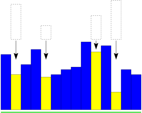
FIG. 2.: The MPEU model. The arrows show the local minima where random amounts of material will be deposited in the next time step.

As mentioned in the Introduction, we know of one example that nature provides with an efficient algorithm for a very large number of processing elements: the human brain with its $10^{11}$ PE-s is the largest parallel computer ever built. Although the intuition suggests that indeed there are scalable parallel schemes, it has only been proved recently, see for details Ref. [1], by using the aforementioned analogy with the simple MPEU surface growth model. While the MPEU model exactly mimics the evolution of the simulated time-horizon, it can also be considered as a primitive model for ion sputtering of surfaces (etching dynamics): to see this, define a new height variable via $h_{i}\equiv-\tau_{i}$, i.e. flip Figure 2 upside down. This means that instead of depositing material we have to take, ‘etch’, and this has to be done at the local maxima of the $\{h_{i}\}$ surface. In sputtering of surfaces by ion bombardement an incoming ion-projectile will most likely ‘break off’ a piece from the top of a mound instead from a valley, very similar to our ‘reversed’ MPEU model. It was shown that the sputtering process is described by the KPZ equation, [22, 14]. This qualitative argument is in complete agrrement with the extensive MC simulations and a coarse-grained approximation of Ref. [1] that MPEU, similar to the single-step model, it also belongs to the KPZ dynamic universality class; in one dimension the macroscopic landscape is governed by the EW Hamiltonian.

The slope varaibles $\phi_{i}$ for MPEU are not independent in the $L\rightarrow\infty$ limit, but short-ranged. This already guarantees that the steady-state behavior is governed by the EW Hamiltonian, and the density of local minima does not vanish in the thermodynamic limit. Our results confirm that the finite-size effects for $\langle u\rangle$ follow eq. (28):

$$\langle u\rangle_{L}\simeq\langle u\rangle_{\infty}+\frac{\rm const.}{L}$$ (52)

with $\langle u\rangle_{\infty}=0.24641(7)$, see Fig. 3.

FIG. 3.: Density of minima vs. $1/L$ for the MPEU model.

We conclude that the basic algorithm (one site per PE) is scalable for one-dimensional arrays. The same correspondence can be applied to model the performance of the algorithm for higher-dimensional logical PE topologies. While this will involve the typical difficulties of surface-growth modeling, such as an absence of exact results and very long simulation times, it establishes potentially fruitful connections between two traditionally separate research areas.

C The larger curvature model

In this subsection we briefly present a curvature driven SOS surface deposition model known in the literature as the larger curvature model, and show a numerical analysis of the density of minima on this model. This model was originally introduced by Kim and Das Sarma [26] and Krug [27] independently, as an atomistic deposition model which fully conforms to the behaviour of the continuum fourth order linear Mullins equation ($\nu=0$, $\kappa>0$ in Eq. 4). Note that the discrete analysis we presented in Section II is based on the discretization of the continuum equation using the simplest forward Euler differencing scheme. The larger curvature model, however, is a growth model where the freshly deposited particles diffuse on the surface according to the rules of the model until they are embedded. Since in all the quantities studied so far, the correspondence (on the level of scaling) between the larger curvature model and the Langevin equation is very good, we would expect that the dynamic scaling properties of the density of minima for both the model and the equation to be identical.

The large curvature model has rather simple rules: a freshly deposited atom (let us say at site $i$) will be incorporated at the nearest neighbor site which has largest curvature (i.e., $K_{i}=h_{i+1}+h_{i-1}-2h_{i}$ is maximum). If there are more neighbors with the same maximum curvature, then one is chosen randomly. If the original site ($i$) is among those with maximum curvature, then the atom is incorporated at $i$.

Figure 4 shows the scaling of the density of minima $<u>_{L}$ in the steady state, vs. $1/\sqrt{L}$. According to Eq. (32), for the fourth order equation on the lattice, the behavior of the density of minima in the steady state scales with system size as $1/\sqrt{L}$. And indeed, Figure 4 shows the same behaviour for the larger curvature model, as expected. Note that this behavior sets in at rather small system sizes already, at about $L=100$, meaning that the finite system size effects are rather small for the larger curvature model. This is a very fortunate property since increasing the system size means decreasing the density of minima, therefore relative statistical errors will increase.

FIG. 4.: Density of minima in the steady state for the larger curvature model.

This can only be improved by better statistics, i.e., with averages over larger number of runs. This becomes however quickly a daunting task, since the cross-over time toward the steady state scales with system size as $L^{4}$. As we shall see in Section V.A, a matematically rigorous approach to the continuum equation yields the same $1/\sqrt{L}$ behaviour. Since the density of minima does decay to zero, an algorithm corresponding to the larger curvature model (or the Mullins equation) would not be asymptotically scalable.

Finally, we would like to make a brief note about the observed morphologies in the steady state for the Mullins equation , or the related models. It has been shown previously [28] that in the steady state the morphology tipically shows a single large mound (or macroscopic groove). At first sight this may appear as a surprise, since we have shown that the number of minima (or maxima) diverges as $\sqrt{L}$ (the density vanishes as $1/\sqrt{L}$. There is however no contradiction, because that refers to a a mound that expands throughout the system, i.e. it is a long wavelenght structure, whereas the number of minima measures all the minima, and thus it is a short wavelenght characteristic. In the steady state we indeed have a single large, macroscopic groove, however, there are numerous small dips and humps generated by the constant coupling to the noise.

IV Extremal-point densities on the continuum

Let us consider a continuous and at least two times differentiable function $f:[0,L]\to{\mathbb{R}}$. We are interested in counting the total number of extrema of $f$ in the $[0,L]$ interval. The topology of continuous curves in one dimension allows for three possibilities on the nature of a point $x_{i}$ for which $f^{\prime}|_{x_{i}}=0$. Namely, $x_{i}$ is a local minimum if $f^{\prime\prime}|_{x_{i}}>0$, a local maximum if $f^{\prime\prime}|_{x_{i}}<0$ and it is degenerate if $f^{\prime\prime}|_{x_{i}}=0$. We call the point $x_{i}$ a degenerate flat of order $k$, if $f^{(j)}|_{x_{i}}=0$ for $j=1,2,..,k$ and $f^{(k+1)}|_{x_{i}}\neq 0$, $k\geq 2$, assuming that the higher order derivatives $f^{(j)}$ implied exist. The counter-like quantity

$$c(L,[f])\equiv\frac{1}{L}\int\limits_{0}^{L}dx\;|f^{\prime\prime}|\;\delta(f^{\prime})$$ (53)

where $\delta$ is the Dirac-delta, gives the number of extremum points per unit length in the interval $[0,L]$, which in the limit of $L\to 0$ is the extremum point density of $f$ in the origin. For our purposes $L$ will always be a finite number, however, for the sake of briefness we shall refer to $c$ simply as the density of extrema. Note that counting the extrema of a function $f$ is equivalent to counting the zeros of its derivate $f^{\prime}$. The divergence of $c$ for finite $L$ implies either the existence of completely flat regions (infinitely degenerate), or an “infinitely wrinkled” region, such as for the truncated Weierstrass function shown in Fig. 2 ( in this latter case the divergence is understood by taking the limit $M\to\infty$). As already explained in the Introduction this infinitely wrinkled region does not necessarily imply that the curve is fractal, but if the curve is fractal, then regions of infinite wrinkledness must exist. The divergence or non-divergence of $c$ can be used as an indicator of the existence of such regions (completely flat or infinitely wrinkled).

One can make the following precise statement related to the counter $c$: if $x_{i}$ is an extremum point of $f$ of at most finite degeneracy $k$, and if there exist a small enough $\epsilon$, such that $f$ is analytic in the neighborhood $[x_{i}-\epsilon,x_{i}+\epsilon]$, and there are no other extrema in this neighborhood, then

$$I(x_{i})\equiv\int\limits_{x_{i}-\epsilon}^{x_{i}+\epsilon}dx\;|f^{\prime\prime}|\;\delta(f^{\prime})=1\;,\;\;\;0<\epsilon\ll 1$$ (54)

In the following we give a proof to this statement.

Using Taylor-series expansions around $x_{i}$, one writes:

$$f^{\prime}(x)=\frac{a_{k}}{k!}(x-x_{i})^{k}+\frac{a_{k+1}}{(k+1)!}(x-x_{i})^{k+1}+...$$ (55)

$$f^{\prime\prime}(x)=\frac{a_{k}}{(k-1)!}(x-x_{i})^{k-1}+\frac{a_{k+1}}{k!}(x-x_{i})^{k}+...$$ (56)

where we introduced the shorthand notation $a_{j}\equiv f^{(j+1)}|_{x_{i}}$. For the non-degenerate case of $k=1$, (54) follows from a classical property of the delta function, namely:

$$\delta(g(x))=\sum_{i}|g^{\prime}(x_{i})|^{-1}\;\delta(x-x_{i})\;,\;\;\;\mbox{ $x_{i}$ are {\em simple} zeros of $g$}.$$ (57)

Let us now assume that $x_{i}$ is degenerate of order $k$ ($k\geq 2$). Using the expansions (55), (56), the variable change $u=x-x_{i}$, and the well-known property $\delta(ax)=|a|^{-1}\delta(x)$, we obtain:

$$I(x_{i})=k\int\limits_{-\epsilon}^{\epsilon}du\;|u|^{k-1}\;\left|1+\sum_{j=1}^{\infty}\frac{(k-1)!}{(k-1+j)!}\;\frac{a_{k+j}}{a_{k}}\;u^{j}\right|\;\delta\left(|u|^{k}\left[1+\sum_{j=1}^{\infty}\frac{k!}{(k+j)!}\;\frac{a_{k+j}}{a_{k}}\;u^{j}\right]\right)$$ (58)

Next we split the integral (58) in two: $\int_{-\epsilon}^{\epsilon}...=\int_{-\epsilon}^{0}...+\int_{0}^{\epsilon}$, make the variable change $u\to-u$ in the first one, and then $z=u^{k}$ in both integrals. The final expression can then be written in the form:

$$I(x_{i})=\int\limits_{-\epsilon^{k}}^{\epsilon^{k}}dz\;|A(z)|\;\delta(zB(z))\;,$$ (59)

where

$$A(z)=1+\sum_{j=1}^{\infty}\frac{(k-1)!}{(k-1+j)!}\;\frac{a_{k+j}}{a_{k}}\;z^{j}|z|^{\frac{j}{k}-j}\;,\;\;\;\mbox{and}\;\;\;B(z)=1+\sum_{j=1}^{\infty}\frac{k!}{(k+j)!}\;\frac{a_{k+j}}{a_{k}}\;z^{j}|z|^{\frac{j}{k}-j}$$ (60)

We have $A(0)=B(0)=1$, and

$$[zB(z)]^{\prime}=1+\sum_{j=1}^{\infty}\frac{k!}{(k+j)!}\;\frac{a_{k+j}}{a_{k}}\;\left(\frac{j}{k}+1\right)z^{j}|z|^{\frac{j}{k}-j}\;,\;\;\;\rightarrow\;\;\;\left.[zB(z)]^{\prime}\right|_{z=0}=1\;.$$ (61)

(Take the derivatives separately to the right and to the left of $z=0$). Thus, since $z=0$ is a simple zero of $zB(z)$, property (57) can be applied for sufficiently small $\epsilon$:

$$I(x_{i})=|A(0)|=1$$ (62)

proving our assertion. Note that because of (54), $c$ counts all the non-degenerate and the finitely degenerate points as well, giving the equal weight of unity to each. Can we count the non-degenerate extrema separately? The answer is affirmative, if one considers instead of (53) the following quantity:

$$c_{q}(L,[f])\equiv\frac{1}{L}\int\limits_{0}^{L}dx\;|f^{\prime\prime}|^{q+1}\;\delta(f^{\prime})\;,\;\;\;q>0$$ (63)

Performing the same steps as above we obtain for a degenerate point:

$$I_{q}(x_{i})\equiv\int\limits_{x_{i}-\epsilon}^{x_{i}+\epsilon}dx\;|f^{\prime\prime}|^{q+1}\;\delta(f^{\prime})=\left[\frac{|a_{k}|}{(k-1)!}\right]^{q}\int\limits_{-\epsilon^{k}}^{\epsilon^{k}}dz\;|z|^{q\left(1-\frac{1}{k}\right)}\;|A(z)|^{q+1}\;\delta(zB(z))\;.$$ (64)

Since $k\geq 2$, $q\left(1-\frac{1}{k}\right)\geq\frac{1}{2}q>0$, i.e.,

$$I_{q}(x_{i})=0\;,\;\;\;\mbox{for $x_{i}$ degenerate}.$$ (65)

This means, that $q>0$ eliminates the degenerate points from the count. To non-degenerate points ($k=1$) (63) gives the weight of

$$I_{q}(x_{i})=|a_{1}|^{q}=\Big{|}f^{\prime\prime}|_{x_{i}}\Big{|}^{q}\;,\;\;\;\mbox{for $x_{i}$ non-degenerate}.$$ (66)

In other words,

$$c_{q}(L,[f])=\frac{1}{L}\sum_{i}\left|K(x_{i})\right|^{q}\;,\;\;\;\mbox{$q>0$, $x_{i}$ non-degenerate extrema of $f$}$$ (67)

where $K(x)=f^{\prime\prime}$ is the curvature of $f$ at $x$. The limit $q\to 0^{+}$ in (67) gives the extremum point density $\overline{c}(L,[f])$ of $f$ of non-degenerate extrema:

$$\overline{c}(L,[f])=\lim_{q\to 0^{+}}c_{q}(L,[f])=\lim_{q\to 0^{+}}\frac{1}{L}\int\limits_{0}^{L}dx\;|f^{\prime\prime}|^{q+1}\;\delta(f^{\prime})$$ (68)

It is important to note, that taking the $q\to 0^{+}$ limit in (67) is not equivalent to taking $q=0$ in (63), i.e., the limit and the integral on the rhs of (68) are not interchangeable! The difference is the set of degenerate points!

Until now, we did not make any distiction between maxima and minima. In a natural way, we expect that the quantity:

$$u(L,[f])\equiv\frac{1}{L}\int\limits_{0}^{L}dx\;f^{\prime\prime}\;\delta(f^{\prime})\;\theta(f^{\prime\prime})$$ (69)

where $\theta(x)$ is the Heaviside step-function, will give the density of minima (due to the step function, here we can drop the absolute values). However, performing a similar derivation as above, one concludes that (69) is a little bit ill-defined, in the sense that the weight given to degenerate points depends on the definition of the step-function in the origin (however, $u(L,[f])$ is bounded). Introducing a $q-regulator$ as above, the weight of degenerate points is pulled down to zero:

$$u_{q}(L,[f])\equiv\frac{1}{L}\int\limits_{0}^{L}dx\;[f^{\prime\prime}]^{q+1}\;\delta(f^{\prime})\;\theta(f^{\prime\prime})\;,\;\;\;q>0.$$ (70)

and

$$u_{q}(L,[f])=\frac{1}{L}\sum_{i}\left[K(x_{i})\right]^{q}\;,\;\;\;\mbox{$q>0$, $x_{i}$ non-degenerate minima of $f$}$$ (71)

Note that in the equation above the absolute values are not needed, since we are summing over the curvatures of all local minima. The density $\overline{u}(L,[f])$ of non-degenerate minima of $f$ is obtained after taking the limit $q\to 0^{+}$:

$$\overline{u}(L,[f])=\lim_{q\to 0^{+}}u_{q}(L,[f])$$ (72)

and the limit is not interchangeable with the integral in (70). To obtain densities for maxima, one only has to replace the argument $f^{\prime\prime}$ of the Heaviside function with $-f^{\prime\prime}$.

A Stochastic extremal-point densities

We are interested to explore the previously introduced quantities for a stochastic function, subject to time evolution, $h(x,t)$. This function may be for example the solution to a Langevin equation. We define the two basic quantities in the same way as before, except that now one performs a stochastic average over the noise, as well:

$$C_{q}(L,t)=\left\langle\frac{1}{L}\int\limits_{0}^{L}dx\;\left|\frac{\partial^{2}h}{\partial x^{2}}\right|^{q+1}\delta\left(\frac{\partial h}{\partial x}\right)\right\rangle\;,\;\;\;\mbox{and}\;\;\;U_{q}(L,t)=\left\langle\frac{1}{L}\int\limits_{0}^{L}dx\;\left[\frac{\partial^{2}h}{\partial x^{2}}\right]^{q+1}\delta\left(\frac{\partial h}{\partial x}\right)\;\theta\left(\frac{\partial^{2}h}{\partial x^{2}}\right)\right\rangle$$ (73)

For systems preserving translational invariance, the stochastic average of the integrand becomes $x$-independent, and the integrals can be dropped:

$$C_{q}(L,t)=\left\langle\left|\frac{\partial^{2}h}{\partial x^{2}}\right|^{q+1}\delta\left(\frac{\partial h}{\partial x}\right)\right\rangle$$ (74)

$$U_{q}(L,t)=\left\langle\left[\frac{\partial^{2}h}{\partial x^{2}}\right]^{q+1}\delta\left(\frac{\partial h}{\partial x}\right)\;\theta\left(\frac{\partial^{2}h}{\partial x^{2}}\right)\right\rangle$$ (75)

According to (67) and (71), $C_{q}(L,t)$ and $U_{q}(L,t)$ can be thought of as time dependent “partition functions” for the non-degenerate extremal-point densities of the underlying stochastic process, with $q$ playing the role of “inverse temperature”:

$$C_{q}(L,t)=\left\langle\frac{1}{L}\sum_{i}\left|K(x_{i})\right|^{q}\right\rangle\;,\;\;\;\mbox{$q>0$, $x_{i}$ non-degenerate extrema}$$ (76)

$$U_{q}(L,t)=\left\langle\frac{1}{L}\sum_{i}\left[K(x_{i})\right]^{q}\right\rangle\;,\;\;\;\mbox{$q>0$, $x_{i}$ non-degenerate minima}$$ (77)

It is important to mention that in the above equations the average $<..>$ and the summation are not interchangeable: particular realizations of $h$ have particular sets of minima.

Two values for $q$ are of special interest: when $q\to 0^{+}$ and $q=1$. In the first case we obtain the stochastic average of the density of non-degenerate extrema and minima:

$$\overline{C}(L,t)=\lim_{q\to 0^{+}}C_{q}(L,t)\;,\;\;\;\mbox{and}\;\;\;\overline{U}(L,t)=\lim_{q\to 0^{+}}U_{q}(L,t)\;,$$ (78)

and in the second case we obtain the stochastic average of the mean curvature at extrema and minima:

$$\overline{K}_{ext}(L,t)=\frac{C_{1}(L,t)}{\overline{C}(L,t)}\;,\;\;\;\mbox{and}\;\;\;\overline{K}_{min}(L,t)=\frac{U_{1}(L,t)}{\overline{U}(L,t)}\;,$$ (79)

(we need to normalize with the number of extrema/minima per unit length to get the curvature per extremum/minimum).

In the following we explore the quantities (74)-(79) for a large class of linear Langevin equations. To simplify the calculations, we will assume that $q$ is a positive integer. Then we will attempt analytic continuation on the final result as a function of $q$. In the calculations we will make extensive use of the standard integral representations of the delta and step functions:

$$\delta(y)=\int\limits_{-\infty}^{\infty}\frac{dz}{2\pi}\;e^{izy}=\sum_{n=0}^{\infty}\int\limits_{-\infty}^{\infty}\frac{dz}{2\pi}\;\frac{(iz)^{n}}{n!}\;y^{n}\;,$$ (80)

$$\theta(y)=\lim_{\epsilon\to 0^{+}}\int\limits_{-\infty}^{\infty}\frac{dz}{2\pi}\;\frac{e^{izy}}{\epsilon+iz}=\lim_{\epsilon\to 0^{+}}\sum_{n=0}^{\infty}\int\limits_{-\infty}^{\infty}\frac{dz}{2\pi}\;\frac{1}{\epsilon+iz}\;\frac{(iz)^{n}}{n!}\;y^{n}$$ (81)

If $q$ is a positive integer, we may drop the absolute value signs in (75). In (74) we can only do that for odd $q$. The absolute values make the calculation of stochastic averages very difficult. We can get around this problem by employing the following identity:

$$|y|^{n}=y^{n}\left\{(-1)^{n}+\theta(y)\left[1-(-1)^{n}\right]\right\}$$ (82)

This brings (74) to

$$C_{q}(L,t)=\left[1-(-1)^{q}\right]U_{q}(L,t)+(-1)^{q+1}B_{q}(L,t)$$ (83)

where

$$B_{q}(L,t)=\left\langle\frac{1}{L}\int\limits_{0}^{L}dx\;\left(\frac{\partial^{2}h}{\partial x^{2}}\right)^{q+1}\delta\left(\frac{\partial h}{\partial x}\right)\right\rangle=\left\langle\left(\frac{\partial^{2}h}{\partial x^{2}}\right)^{q+1}\delta\left(\frac{\partial h}{\partial x}\right)\right\rangle$$ (84)

Obviously for $q$ odd integer, $B_{q}=C_{q}$. For $q$ even, $B_{q}$ is an interesting quantity by itself. In this case the weight of an extremum $x_{i}$ is $sgn(K(x_{i}))|K(x_{i})|^{q}$. If the analytic continuation can be performed, then the $q\to 0^{+}$ limit will tell us if there are more non-degenerate maxima than minima (or otherwise) in average. Using the integral representations (80) and (81):

$$B_{q}(L,t)=\sum_{n=0}^{\infty}\int\limits_{-\infty}^{\infty}\frac{dz}{2\pi}\;\frac{(iz)^{n}}{n!}\;\left\langle\left(\frac{\partial^{2}h}{\partial x^{2}}\right)^{q+1}\left(\frac{\partial h}{\partial x}\right)^{n}\right\rangle$$ (85)

$$U_{q}(L,t)=\lim_{\epsilon\to 0^{+}}\sum_{n_{1}=0}^{\infty}\sum_{n_{2}=0}^{\infty}\int\limits_{-\infty}^{\infty}\frac{dz_{1}}{2\pi}\;\frac{(iz_{1})^{n_{1}}}{n_{1}!}\int\limits_{-\infty}^{\infty}\frac{dz_{2}}{2\pi}\;\frac{(iz_{2})^{n_{2}}}{n_{2}!}\;\frac{1}{\epsilon+iz_{2}}\;\left\langle\left(\frac{\partial^{2}h}{\partial x^{2}}\right)^{n_{2}+q+1}\left(\frac{\partial h}{\partial x}\right)^{n_{1}}\right\rangle$$ (86)

V Extremal-point densities of linear stochastic evolution equations

Next we calculate the densities (85), (86) for the following type of linear stochastic equations:

$$\frac{\partial h}{\partial t}=-\nu\left(-\nabla^{2}\right)^{z/2}h+\eta(x,t)\;,\;\;\;\;\nu,D,z>0\;,\;\;\;x\in[0,L]$$ (87)

with initial condition $h(x,0)=0$, for all $x\in[0,L]$. $\eta$ is a white noise term drawn from a Gaussian distribution with zero mean $\langle\eta(x,t)\rangle=0$, and covariance :

$$\langle\eta(x,t)\eta(x^{\prime},t^{\prime})\rangle=2D\delta(x-x^{\prime})\;\delta(t-t^{\prime})\;,$$ (88)

We also performed our calculations with other noise types, such as volume conserving and long-range correlated, however the details are to lengthy to be included in the present paper, it will be the subject of a future publication. As boundary condition we choose periodic boundaries:

$$h(x+nL,t)=h(x,t)\;,\;\;\;\eta(x+nL,t)=\eta(x,t)\;,\;\;\;\mbox{for all $n\in{\mathbb{Z}}$}$$ (89)

The general solution to (87) is obtained simply with the help of Fourier series [18]. The Fourier series and its coefficients for a function $f$ defined on $[0,L]$ is

$$f(x)=\sum_{k}\tilde{f}(k)\;e^{ikx}\;,\;\;\;\tilde{f}(k)=\frac{1}{L}\int\limits_{-L}^{L}dx\;f(x)\;e^{-ikx}$$ (90)

where $k=\frac{2\pi}{L}n$, $n=..,-2,-1,0,1,2,..$. The Fourier coefficients of the general solution to (87) are:

$$\tilde{h}(k,t)=\int\limits_{0}^{t}dt^{\prime}\;e^{-\nu|k|^{z}(t-t^{\prime})}\tilde{\eta}(k,t^{\prime})$$ (91)

The correlations of the noise in momentum space are:

$$\left\langle\tilde{\eta}(k,t)\tilde{\eta}(k^{\prime},t^{\prime})\right\rangle=\frac{2D}{L}\;\delta_{k,-k^{\prime}}\;\delta(t-t^{\prime})\;.$$ (92)

Due to the Gaussian character of the noise, the two-point correlation of the solution (91) is also delta-correlated and it completely characterizes the statistical properties of the stochastic dynamics (87). It is given by:

$$\left\langle\tilde{h}(k,t)\tilde{h}(k^{\prime},t^{\prime})\right\rangle=S(k,t)\delta_{k,-k^{\prime}}$$ (93)

where $S(k,t)$ is the structure factor given by:

$$S(k,t)=\frac{D}{\nu L|k|^{z}}\left[1-e^{-2\nu|k|^{z}t}\right]\;.$$ (94)

Equation (87) has been analyzed in great detail by a number of authors, see Ref. [18] for a review. It was shown that there exist un upper critical dimension $d_{c}=z$ for the noisy case of Eq. (87) which separates the rough regime with $d<z$ from the non-roughening regime $d>z$. In one dimension, the rough regime corresponds to the condition $z>1$, which we shall assume from now on, since this is where the interesting physics lies.

Next, we evaluate the quantities (74)-(79) via directly calculating the expressions in (85) and (86). This amounts to computing averages of type:

$$Q_{N,M}=\left\langle\left(\frac{\partial^{2}h}{\partial x^{2}}\right)^{N}\left(\frac{\partial h}{\partial x}\right)^{M}\right\rangle$$ (95)

Expressing $h$ with its Fourier series according to (90), we write:

$$\left(\frac{\partial h}{\partial x}\right)^{M}=i^{M}\sum_{k_{1}}...\sum_{k_{M}}k_{1}...k_{M}\;\tilde{h}(k_{1},t)...\tilde{h}(k_{M},t)\;e^{i(k_{1}+...+k_{M})x}$$ (96)

$$\left(\frac{\partial^{2}h}{\partial x^{2}}\right)^{N}=(-1)^{N}\sum_{k_{1}^{\prime}}...\sum_{k_{N}^{\prime}}{k_{1}^{\prime}}^{2}...{k_{N}^{\prime}}^{2}\;\tilde{h}(k_{1}^{\prime},t)...\tilde{h}(k_{N}^{\prime},t)\;e^{i(k_{1}^{\prime}+...+k_{N}^{\prime})x}$$ (97)

which then is inserted in (95). Thus in Fourier space one needs to calculate averages of type $\langle\tilde{h}(k_{1},t)...\tilde{h}(k_{M},t)\tilde{h}(k_{1}^{\prime},t)...\tilde{h}(k_{N}^{\prime},t)\rangle$. According to (93) $\tilde{h}$ is anti-delta-correlated, therefore these averages can be performed in the standard way [30] which is by taking all the possible pairings of indices and employing (93). In our case there are three types of pairings: $\{k_{j},k_{l}\}$, $\{k_{j},k_{l}^{\prime}\}$, and $\{k_{j}^{\prime},k_{l}^{\prime}\}$. Let us pick a ‘mixed’ pair $\{k_{j},k_{l}^{\prime}\}$ containing a primed and a non-primed index. The corresponding contribution in the $Q_{N,M}$ will be:

$$\sum_{k_{j}}\sum_{k_{l}^{\prime}}k_{j}{k_{l}^{\prime}}^{2}S(k_{l}^{\prime},t)e^{i(k_{j}+k_{l}^{\prime})x}\delta_{k_{j},-k_{l}^{\prime}}$$ (98)

Since the structure factor $S(k,t)$ is an even function in $k$, (98) becomes $\sum_{k_{j}}{k_{j}}^{3}S(k_{j},t)=0$, because the summand is an odd function of $k_{j}$ and the summation is symmetric around zero. Thus, it is enough to consider non-mixed index-pairs, only. This means, that $Q_{N,M}$ decouples into:

$$Q_{N,M}=\left\langle\left(\frac{\partial^{2}h}{\partial x^{2}}\right)^{N}\right\rangle\left\langle\left(\frac{\partial h}{\partial x}\right)^{M}\right\rangle$$ (99)

The averages are calculated easily, and we find:

$$\left\langle\left(\frac{\partial h}{\partial x}\right)^{M}\right\rangle=\left\{\begin{array}[]{l}(M-1)!!\;\left[\phi_{2}(L,t)\right]^{M/2}\;,\;\;\;\mbox{for $M$ even }\;,\\ \\ 0\;,\;\;\;\mbox{for $M$ odd }\end{array}\right.$$ (103)

and

$$\left\langle\left(\frac{\partial^{2}h}{\partial x^{2}}\right)^{N}\right\rangle=\left\{\begin{array}[]{l}(N-1)!!\;\left[\phi_{4}(L,t)\right]^{N/2}\;,\;\;\;\mbox{for $N$ even }\;,\\ \\ 0\;,\;\;\;\mbox{for $M$ odd }\end{array}\right.$$ (107)

where

$$\phi_{m}(L,t)\equiv\sum_{k}|k|^{m}\;S(k,t)$$ (108)

Employing (103), and (107) in (85), it follows that if $q$ is an even integer, $q=2s$, $s=1,2,..$:

$$B_{2s}(t)=0\;,\;\;\;s=1,2,...$$ (109)

whereas for $q$ odd integer, $q=2s-1$, $s=1,2,..$:

$$B_{2s-1}(t)=C_{2s-1}(t)=\frac{2^{s-\frac{1}{2}}}{\pi}\;\Gamma\left(s+\frac{1}{2}\right)\;\frac{\left[\phi_{4}(L,t)\right]^{s}}{\sqrt{\phi_{2}(L,t)}}\;,\;\;\;s=1,2,...$$ (110)

where we used the identity $2^{p}(2p-1)!!/(2p)!=1/p!$, and performed the Gaussian integral.

The calculation of $U_{q}$ is a bit trickier. The sum over $n_{1}$ in (86) is easy and leads to the Gaussian $e^{-\phi_{2}(L,t)z_{1}^{2}/2}$. However, the sum over $n_{2}$ is more involved. Let us make the temporary notation for the sum over $n_{2}$:

$$R_{q}=\sum_{n_{2}=0}^{\infty}\frac{(iz_{2})^{n_{2}}}{n_{2}!}\;(2r-1)!!\;\left[\phi_{4}(L,t)\right]^{r}\;,\;\;\;n_{2}+q+1=2r$$ (111)

We have to distinguish two cases according to the parity of $q$:
1) $q$ is odd, $q=2s-1$, $s=1,2,..$. In this case $R_{q}$ becomes

$$R_{2s-1}=\sum_{r=s}^{\infty}\frac{(iz_{2})^{2(r-s)}}{[2(r-s)]!}\;\frac{(2r)!}{r!}\;\left[\frac{1}{2}\phi_{4}(L,t)\right]^{r}=(z_{2})^{-2s}(-1)^{s}\left\{\frac{\partial^{2s}}{\partial x^{2s}}\left[e^{-\phi_{4}(L,t)z_{2}^{2}x^{2}/2}\right]\right\}_{x=1}$$ (112)

The Hermite polynomials are defined via the Rodrigues formula as:

$$H_{n}(x)=(-1)^{n}e^{x^{2}}\frac{d^{n}}{dx^{n}}\left(e^{-x^{2}}\right)$$ (113)

Using this, we can express $R_{2s-1}$ with the help of Hermite polynomials:

$$R_{2s-1}=(-1)^{s}\left[\frac{1}{2}\phi_{4}(L,t)\right]^{s}\;H_{2s}\left(\sqrt{\frac{1}{2}\phi_{4}(L,t)}z_{2}\right)\;e^{-\phi_{4}(L,t)z_{2}^{2}x^{2}/2}$$ (114)

2) $q$ is even, $q=2s$, $s=1,2,..$. The calculations are analogous to the odd case:

$$R_{2s}=\sum_{r=s+1}^{\infty}\frac{(iz_{2})^{2(r-s)-1}}{[2(r-s)-1]!}\;\frac{(2r)!}{r!}\;\left[\frac{1}{2}\phi_{4}(L,t)\right]^{r}=(iz_{2})^{-2s-1}\left\{\frac{\partial^{2s+1}}{\partial x^{2s+1}}\left[e^{-\phi_{4}(L,t)z_{2}^{2}x^{2}/2}\right]\right\}_{x=1}$$ (115)

or via Hermite polynomials:

$$R_{2s}=i(-1)^{s}\left[\frac{1}{2}\phi_{4}(L,t)\right]^{s+\frac{1}{2}}\;H_{2s+1}\left(\sqrt{\frac{1}{2}\phi_{4}(L,t)}z_{2}\right)\;e^{-\phi_{4}(L,t)z_{2}^{2}x^{2}/2}$$ (116)

In order to obtain $U_{q}$ we have to do the integral over $z_{2}$ in (86). This can be obtained after using the formula:

$$\int\limits_{-\infty}^{\infty}dx\;(x\pm ic)^{\nu}\;H_{n}(x)\;e^{-x^{2}}=2^{n-1-\nu}\sqrt{\pi}\;\frac{\Gamma\left(\frac{n-\nu}{2}\right)}{\Gamma(-\nu)}\;e^{\pm\frac{i\pi}{2}(\nu+n)}\;,\;\;\;c\to 0^{+}.$$ (117)

Finally, the densities for the minima read as:

$$U_{2s}(t)=\frac{2^{s-1}}{\pi}\;\Gamma(s+1)\;\frac{\left[\phi_{4}(L,t)\right]^{s+\frac{1}{2}}}{\sqrt{\phi_{2}(L,t)}}$$ (118)

$$U_{2s-1}(t)=\frac{2^{s-\frac{3}{2}}}{\pi}\;\Gamma\left(s+\frac{1}{2}\right)\;\frac{\left[\phi_{4}(L,t)\right]^{s}}{\sqrt{\phi_{2}(L,t)}}$$ (119)

Formulas (109), (110), (118), and (119) combined with (83) can be condensed very simply, and we obtain the general result as:

$$U_{q}(L,t)=\frac{2^{\frac{q}{2}-1}}{\pi}\;\Gamma\left(\frac{q}{2}+1\right)\;\frac{\left[\phi_{4}(L,t)\right]^{\frac{q+1}{2}}}{\sqrt{\phi_{2}(L,t)}}$$ (120)

$$C_{q}(L,t)=2U_{q}(L,t)$$ (121)

Equations (120), (121) with together with (119) fully solve the problem for the density of non-degenerate extrema. Eq. (121) is an expected result in one dimension, because Eq. (87) preserves the up-down symmetry. The density of non-degenerate minima is:

$$\overline{U}(L,t)=\lim_{q\to 0^{+}}U_{q}(L,t)=\frac{1}{2\pi}\;\sqrt{\frac{\phi_{4}(L,t)}{\phi_{2}(L,t)}}$$ (122)

and the stochastic average of the mean curvature at a minimum point is:

$$\overline{K}(L,t)=\frac{U_{1}(L,t)}{\overline{U}(L,t)}=\sqrt{\frac{\pi}{2}}\;\sqrt{\phi_{4}(L,t)}$$ (123)

i.e., the average curvature at a minimum is proportional to the square root of the fourth moment of the structure factor. In the following section we exploit the physical information behind the above expressions for the stochastic process (87). At some parameter values a few, or all the quantities above may diverge. In this case we introduce a microscopic lattice cut-off $0<a\ll 1$, and analyze the limit $a\to 0^{+}$ in the final formulas. This in fact corresponds to placing the whole problem on a lattice with lattice constant $a$. It has been shown in Ref. [18] that for the class of equations (87) there are three important length-scales that govern the statistical behavior of the interface $h$: the lattice constant $a$, the system size $L$, and the dynamical correlation length $\xi$ defined by:

$$\xi(t)\equiv(2\nu t)^{1/z}$$ (124)

According to (108) and (94) the function $\phi_{m}(L,t)$ becomes:

$$\phi_{m}(L,t)=\frac{2D}{\nu L}\sum_{n=0}^{\infty}\left(\frac{2\pi n}{L}\right)^{m-z}\left[1-e^{\textstyle-\left(\xi\frac{2\pi n}{L}\right)^{z}}\right]\;,\;\;\;m=2,4$$ (125)

The $n=0$ term can be dropped from the sum above, because it is zero even for $m<z$ (expand the exponential and then take $n=0$). However, the whole sum may diverge depending on $m$ and $z$. In order to handle all the cases, including the divergent ones we introduce a microscopic lattice cut-off $a$, $0<a\ll 1$, and then analyze the limit $a\to 0^{+}$ in the final expressions. This is in fact equivalent to putting the whole problem on a lattice of lattice spacing $a$. Appropiately, (125) becomes:

$$\phi_{m}(L,t)=\frac{2D}{\nu L}\sum_{n=1}^{\frac{L}{2a}}\left(\frac{2\pi n}{L}\right)^{m-z}\left[1-e^{\textstyle-\left(\xi\frac{2\pi n}{L}\right)^{z}}\right]\;,\;\;\;m=2,4$$ (126)

A Steady-state regime.

Putting $\xi=\infty$ in (126) $\phi_{m}$ takes a simpler form:

$$\phi_{m}(L,\infty)=\frac{2D}{\nu L}\left(\frac{2\pi}{L}\right)^{m-z}\sum_{n=1}^{\frac{L}{2a}}n^{m-z}\;,\;\;\;m=2,4$$ (127)

As $a\to 0^{+}$, $\phi_{m}$ becomes proportional to $\zeta(z-m)$. For $z-m>1$ $\phi_{m}$ is convergent, otherwise it is divergent. In the divergent case we quote the following results:

$$\sum_{n=1}^{N}n^{s}=\ln{N}+{\cal C}+{\cal O}(1/N)\;,\;\;\;\mbox{if}\;\;s=-1$$ (128)

and

$$\sum_{n=1}^{N}n^{s}=\frac{N^{s+1}}{s+1}\Big{[}1+{\cal O}(1/N)\Big{]}\;,\;\;\;\mbox{if}\;\;s>-1$$ (129)

which we will use to derive the leading behaviour of the extremal point densities when $L/a\to\infty$. From equations (127), (120), (122) and (123) follows:

$$U_{q}(L,\infty)=\Gamma\left(\frac{q}{2}+1\right)\left(\frac{2D}{\pi\nu}\right)^{\frac{q}{2}}\left(2\pi\right)^{\frac{q}{2}(5-z)}L^{-1-\frac{q}{2}(5-z)}\left[\sum_{n=1}^{L/2a}n^{4-z}\right]^{\frac{q+1}{2}}\left[\sum_{n=1}^{L/2a}n^{2-z}\right]^{-\frac{1}{2}}\;,$$ (130)

$$\overline{U}(L,\infty)=\frac{1}{L}\sqrt{\sum_{n=1}^{L/2a}n^{4-z}\left(\sum_{n=1}^{L/2a}n^{2-z}\right)^{-1}}\;,$$ (131)

and

$$\overline{K}(L,\infty)=\sqrt{\frac{D}{2}\left(2\pi\right)^{5-z}L^{z-5}\sum_{n=1}^{L/2a}n^{4-z}}\;.$$ (132)

The convergency (divergency) properties of the sums in Eqs. (130-132) for $a\to 0^{+}$ generate two critical values for $z$, namely $z=3$ and $z=5$. In the three regions separated by these values we obtain qualitatively different behaviors for the extremal-point densities.

i) $z>5$. All quantities are convergent as $a\to 0^{+}$. We have:

$$U_{q}(L,\infty)=\Gamma\left(\frac{q}{2}+1\right)\left(\frac{2D}{\pi\nu}\right)^{\frac{q}{2}}(2\pi)^{\frac{q}{2}(5-z)}\frac{[\zeta(z-4)]^{\frac{q+1}{2}}}{[\zeta(z-2)]^{\frac{1}{2}}}\;L^{-1+\frac{q}{2}(z-5)}\;,\;\;\;\;z>5$$ (133)

$$\overline{U}(L,\infty)=\frac{1}{L}\sqrt{\frac{\zeta(z-4)}{\zeta(z-2)}}\;,\;\;\;\;$$ (134)

$$\overline{K}(L,\infty)=(2\pi)^{\frac{5-z}{2}}\sqrt{\frac{D}{2\nu}\zeta(z-4)}\;L^{\frac{z-5}{2}}\;,\;\;\;\;$$ (135)

Eq. (134) shows that there are a finite number of minima ($\sqrt{\zeta(z-4)/\zeta(z-2)}$) in the steady state, independently of the system size $L$. ($\overline{U}(L,\infty)$ is the number of minima per unit length, and $L\overline{U}(L,\infty)$ is the number of minima on the substrate of size $L$). The mean curvature $\overline{K}(L,\infty)$ diverges with system size as $L^{(z-5)/2}$. This is consistent with the fact that the system size grows as $L$, the width grows as $L^{(z-1)/2}$, i.e., faster than $L$, and thus the peaks and minima should become sleeker and sharper as $L\to\infty$, expecting diverging curvatures in minima and maxima. However, this is not always true, since the sleekness of the humps and mounds does not necessarily imply large curvatures in minima and maxima if the shape of the humps also changes as $L$ changes, i.e., there is lack of self-affinity. The existence of $z=5$ as a critical value is a non-trivial results coming from the presented analysis.

ii) $z=5$. According to (128), $\phi_{4}(L,\infty)$ diverges logarithmically as $a\to 0^{+}$. One obtains:

$$U_{q}(\infty)\simeq\Gamma\left(\frac{q}{2}+1\right)\left(\frac{2D}{\nu\pi}\right)^{\frac{q}{2}}\frac{1}{\sqrt{\zeta(3)}}\frac{1}{L}\left(\ln{\frac{L}{2a}}+{\cal C}\right)^{\frac{q+1}{2}}\;,$$ (136)

$$\overline{U}(L,\infty)=\frac{1}{\sqrt{\zeta(3)}}\;\frac{1}{L}\sqrt{\ln{\frac{L}{2a}}+{\cal C}}\;\;,$$ (137)

$$\overline{K}(L,\infty)=\sqrt{\frac{D}{2\nu}\left(\ln{\frac{L}{2a}}+{\cal C}\right)}\;.$$ (138)

Eq. (137) shows that the although the density of minima vanishes, the number of minima is no longer a constant but diverges logarithmically with system size $L$. The mean curvature still diverges, but logarithmically, when compared to the power law divergence of (135).

For the mean curvature $\overline{K}(\infty)$ in (132) $z=5$ is the only critical value, since it only depends on $\phi_{4}$. For $z<5$, using Eq. (129) we arrive to the result that the mean curvature in a minimum point approaches to an $L$-independent constant for $L/a\to\infty$ with corrections on the order of $a/L$:

$$\overline{K}(L,\infty)\simeq\left(\frac{\pi}{a}\right)^{\frac{5-z}{2}}\sqrt{\frac{D}{2\nu(5-z)}}\;,\;\;\;z<5$$ (139)

We arrived to the same conclusion in Section II.D when we studied the steady state of the discretized version of the continuum equation. Coincidentally, for $z=4$ the two constant values from (139) and (47) are identical ($a=1$ by definition in (47).

iii) $3<z<5$. In this case $\phi_{4}(L,\infty)\to\infty$ and $\phi_{2}(L,\infty)<\infty$ as $a\to 0^{+}$, and:

$$U_{q}(L,\infty)\simeq\Gamma\left(\frac{q}{2}+1\right)\left(\frac{2D}{\nu\pi}\right)^{\frac{q}{2}}\left(\frac{\pi}{a}\right)^{\frac{q}{2}(5-z)}\left(\frac{1}{2a}\right)^{\frac{5-z}{2}}\frac{L^{-\frac{z-3}{2}}}{(5-z)^{\frac{q+1}{2}}\sqrt{\zeta(z-2)}}\;,$$ (140)

and

$$\overline{U}(L,\infty)\simeq\left(\frac{1}{2a}\right)^{\frac{5-z}{2}}\;\frac{L^{-\frac{z-3}{2}}}{\sqrt{(5-z)\zeta(z-2)}}\;\;,$$ (141)

and the mean curvature is just given by (139).

Comparing Eqs. (133), (136), and (140) we can make an interesting observation: while for $z\geq 5$ the dependence on the system size $L$ is coupled to the ‘inverse temperature’ $q$, for $3<z<5$ the dependence on $L$ decouples from $q$, i.e., it becomes independent of the inverse temperature! Eq. (141) shows that the density of minima vanishes with system size as a power law with an exponent $(z-3)/2$ but the number of minima of the substrate diverges as a power law with an exponent of $(5-z)/2$.

iv) $z=3$. In this case $\phi_{4}(L,\infty)\to\infty$ and $\phi_{2}(L,\infty)\to\infty$ logarithmically as $a\to 0^{+}$. One obtains:

$$U_{q}(L,\infty)\simeq\frac{1}{2\sqrt{2}a}\Gamma\left(\frac{q}{2}+1\right)\left(\frac{\pi D}{\nu a^{2}}\right)^{\frac{q}{2}}\frac{1}{\sqrt{\ln{\frac{L}{2a}}+{\cal C}}}\;,$$ (142)

and

$$\overline{U}(L,\infty)\simeq\frac{1}{2\sqrt{2}a}\frac{1}{\sqrt{\ln{\frac{L}{2a}}+{\cal C}}}\;,$$ (143)

with a logarithmically vanishing density of minima, and the dependence on the system size in (142) is not coupled to $q$.

v) $1<z<3$. Now both $\phi_{4}$ and $\phi_{2}$ diverge as $a\to 0^{+}$. Employing (129), yields:

$$U_{q}(L,\infty)\simeq\frac{1}{2a}\Gamma\left(\frac{q}{2}+1\right)\left(\frac{2D}{\pi\nu}\right)^{\frac{q}{2}}\left(\frac{\pi}{a}\right)^{\frac{q}{2}(5-z)}\frac{\sqrt{3-z}}{(5-z)^{\frac{q+1}{2}}}\;,$$ (144)

and

$$\overline{U}(L,\infty)\simeq\frac{1}{2a}\sqrt{\frac{3-z}{5-z}}\;.$$ (145)

Note, that in leading order, both $U_{q}(L,\infty)$ and the density of minima $\overline{U}(L,\infty)$ become system size independent! The system size dependence comes in as corrections on the order of $a/L$ and higher. The fact that the efficiency of the massively parallel algorithm presented in Section III.B is not vanishing is due precisely to the above phenomenon: the fluctuations of the time horizon in the steady state belong to the $z=2$ class (Edwards-Wilkinson universality), and according to the results under iv), the density of minima (or the efficiency of the parallel algorithm) converges to a non-zero constant, as $L\to\infty$, ensuring the scalability of the algorithm. An algorithm that would map into a $z\geq 3$ class would have a vanishing efficiency with increasing the number of processing elements. In particular, for $z=2$, one obtains from (145) $\overline{U}(L,\infty)\simeq(a2\sqrt{3})^{-1}=0.2886.../a$. Note that the utilization we obtained is somewhat different from the discrete case which was $0.25$. This is due to the fact that this number is non-universal and it may show differences depending on the discretization scheme used, however it cannot be zero.

Another important conclusion can be drawn from the final results enlisted above: at and below $z=5$, all the quantities diverge when $a\to 0^{+}$, and keep $L$ fixed. This means that the higher the resolution the more details we find in the morphology, just as for an infinitely wrinkled, or a fractal-like surface. We call this transition accross $z=5$ a ‘wrinkle’ transition. As shown in the Introduction, wrinkledness can assume two phases depending on whether the curve is a fractal or not and the transition between these two pases may be conceived as a phase transition. However, one may be able to scale the system size $L$ with $a$ such that the quantities calculated will not diverge in this limit. This is possible only in the regime $3<z<5$, when we impose:

$$L^{z-3}a^{(q+1)(5-z)}=const.$$ (146)

This shows that the rescaling cannot be done for all inverse temperatures $q$ at the same time. In particular, for the density of minima and $z=4$, $La=const$.

B Scaling regime

In order to obtain the temporal behavior of the extremal-point densities we will use the Poisson summation formula (B4) from Appendix B on (126). After simple changes of variables in the integrals this leads to:

$$\phi_{m}(L,t)=\frac{D}{\nu L}\left(\frac{\pi}{a}\right)^{m-z}\left[1-e^{-\left(\xi\frac{\pi}{a}\right)^{z}}\right]+\frac{D}{\pi\nu}\xi^{-(m-z+1)}\int\limits_{0}^{\pi\xi/a}dx\;x^{m-z}\left(1-e^{-x^{z}}\right)+$$ (147)

$$\frac{2D}{\pi\nu}\xi^{-(m-z+1)}\sum_{n=1}^{\infty}\int\limits_{0}^{\pi\xi/a}dx\;x^{m-z}\cos{\left(\frac{L}{\xi}nx\right)}\left(1-e^{-x^{z}}\right)$$ (148)

This expression shows, that the scaling properties of the dynamics are determined by the dimensionless ratios $L/\xi$ and $\xi/a$. The scaling regime is defined by $a\ll\xi\ll L$.

As we have seen in the previous section, $\phi_{m}$ is convergent for $z>m+1$ but diverges when $z\leq m+1$, as $a\to 0^{+}$. In the convergent case, the lattice spacing $a$ can be taken as zero, and thus the first term on the rhs. of (148) vanishes and the time dependence of the infinite system-size piece of $\phi_{m}$ (the first integral term in (148)) assumes the clean power-law behaviour of $t^{(z-m-1)/z}$ (with a positive exponent). In the divergent case, however, the non-integral term of (148) does not vanish, and the time-dependence will not be a clean power-law. Even the integral terms will present corrections to the power-law $t^{-(m+1-z)/z}$ (which has now a negative exponent), since the limits for integration contain $\xi$. The first intergal on the rhs of (148) for $z\neq m+1$ can be calculated exactly:

$$\int\limits_{0}^{\pi\xi/a}\!\!dx\;x^{m-z}\left(1-e^{-x^{z}}\right)=\frac{1}{m-z+1}\left(\frac{\pi\xi}{a}\right)^{m-z+1}\!\!-\frac{1}{z}\Gamma\left(\frac{m-z+1}{z}\right)+\frac{1}{z}\Gamma\left(\frac{m-z+1}{z},\left(\frac{\pi\xi}{a}\right)^{z}\right),\;\;z\neq m+1$$ (149)

where $\Gamma(\alpha,x)$ is the incomplete Gamma function. In our case $(\pi\xi/a)^{z}$ is a large number, and therefore we can use the asymptotic representation of $\Gamma(\alpha,x)$ for large $x$, see [32], pp. 951, equation 8.357. According to this, for large $x$, $\Gamma(\alpha,x)\sim x^{\alpha-1}e^{-x}$, i.e., it can become arbitrarily small, with an exponential decay. This term can therefore be neglected from (149), compared to the other two terms, even in the divergent case. Inserting (149) into (148), we will see that also the non-integral piece of (148) can be neglected compared to the term generated by the first on the rhs of (149), since in the scaling regime $a\ll\xi\ll L$, and thus the ratio $a/L$ can be neglected compared to $(m-z+1)^{-1}$. (This is needed only in the divergent regime, $z<m+1$.) Thus, one obtains:

$$\phi_{m}(L,t)\simeq\frac{D}{\pi\nu(m-z+1)}\left(\frac{\pi}{a}\right)^{m-z+1}\!\!-\frac{D}{\pi\nu z}\Gamma\left(\frac{m-z+1}{z}\right)\xi^{z-m-1}\left[1-E_{m}\left(\frac{L}{\xi},\frac{\xi}{a}\right)\right],\;\;z\neq m+1$$ (150)

where

$$E_{m}(\lambda,\rho)=\frac{2z}{\Gamma\left(\frac{m-z+1}{z}\right)}\sum_{n=1}^{\infty}\int\limits_{0}^{\pi\rho}dx\;x^{m-z}\cos{(\lambda nx)}\left(1-e^{-x^{z}}\right),\;\;z\neq m+1$$ (151)

The oscillating terms condensed in $E_{m}$ will give the finite-size corrections, as long as $L/\xi\gg 1$.

The $z=m+1$ case (divergent) can also be calculated, however, instead of (149) now we have:

$$\int\limits_{0}^{\pi\xi/a}\!\!\frac{dx}{x}\;\left(1-e^{-x^{z}}\right)=\ln{\left(\frac{\pi\xi}{a}\right)}+\frac{{\cal C}}{z}-\frac{1}{z}\mbox{Ei}\left(-\left(\frac{\pi\xi}{a}\right)^{z}\right),\;\;z=m+1\;.$$ (152)

where $\mbox{Ei}(x)$ is the exponential integral function. According to the large-$x$ expansion of the exponential integral function, see [32], pp. 935, equation 8.215, $\mbox{Ei}(-x)\sim-x^{-1}e^{-x}$, it is vanishing exponentially fast, thus it can be neglected in the expression of $\phi_{m}$ in the scaling limit:

$$\phi_{m}(L,t)\simeq\frac{D}{\pi\nu}\ln{\left(\frac{\pi\xi}{a}\right)}+\frac{D{\cal C}}{\pi\nu z}+\frac{D}{\pi\nu}F_{m}\left(\frac{L}{\xi},\frac{\xi}{a}\right)\;,\;\;z=m+1$$ (153)

where

$$F_{m}(\lambda,\rho)=2\sum_{n=1}^{\infty}\int\limits_{0}^{\pi\rho}\frac{dx}{x}\;\cos{(\lambda nx)}\left(1-e^{-x^{z}}\right),\;\;z=m+1$$ (154)

Thus in the scaling limit, the temporal behavior of $\phi_{m}$ becomes a logarithmic time dependence plus a constant, as long as $L/\xi\gg 1$.

Observe that for $z<m+1$ the first term on the rhs. of (150), reproduces exactly the diverging term (as $a\to 0^{+}$) of the steady-state expression (127) which can be seen after employing (128) in (127). This means that for $\xi\to\infty$, $E_{m}(L/\xi,\xi/a)$ diverges slower than $\xi^{m+1-z}$ (this is how the saturation occurs). Similarly, for $z=m+1$ the first term on the rhs of (153) (after replacing $\xi$ with $L$ ) reproduces the diverging term (as $a\to 0^{+}$) of the steady-state expression (127) which can be seen after employing (129) in (127). This means, that in the saturation (or steady-state) regime the remaining terms from (153) must behave as $const.+{\cal O}(a/L)+\ln{(L/\xi)}$, as $\xi\to\infty$ while keeping $L$ and $a$ fixed.

Just as in the case of steady-state one has to distinguish 5 cases depending on the values of $z$, with respect to the critical values 3 and 5. For the sake of simplicity of writing, we will omit the arguments of $E_{m}(\lambda,\rho)$ and $F_{m}(\lambda,\rho)$.

i) $z>5$. We have:

$$\phi_{m}(L,t)=\frac{D}{\pi\nu(z-m-1)}\Gamma\left(\frac{m+1}{z}\right)\xi^{z-m-1}(1-E_{m})\;,\;\;\;m=2,4$$ (155)

From Eqs. (120), (122) and (123), it follows:

$$U_{q}(L,t)=\frac{1}{2\pi}\Gamma\left(\frac{q}{2}+1\right)\left(\frac{2D}{\pi\nu}\right)^{\frac{q}{2}}\left[\frac{\Gamma\left(\frac{5}{z}\right)}{z-5}\right]^{\frac{q+1}{2}}\left[\frac{z-3}{\Gamma\left(\frac{3}{z}\right)}\right]^{\frac{1}{2}}[\xi(t)]^{-1-\frac{q}{2}(z-5)}\frac{(1-E_{4})^{\frac{q+1}{2}}}{(1-E_{2})^{\frac{1}{2}}}\;,$$ (156)

$$\overline{U}(L,t)=\frac{1}{2\pi}\sqrt{\frac{(z-3)\Gamma\left(\frac{5}{z}\right)}{(z-5)\Gamma\left(\frac{3}{z}\right)}}\;\left[\xi(t)\right]^{-1}\sqrt{\frac{1-E_{4}}{1-E_{2}}}\;,$$ (157)

and

$$\overline{K}(L,t)=\sqrt{\frac{D\Gamma\left(\frac{5}{z}\right)}{2\nu(z-5)}}\left[\xi(t)\right]^{\frac{z-5}{2}}\sqrt{1-E_{4}}\;$$ (158)

and therefore the time-behaviour is a clean power-law: $U_{q}(L,t)$ decays as $\sim t^{-[2+q(z-5)]/2z}$, $\overline{U}(L,t)\sim t^{-1/z}$, and $\overline{K}(L,t)$ diverges as $\sim t^{(z-5)/2z}$, for $L/\xi\gg 1$.

ii) $z=5$. In this case $\phi_{4}$ takes the form (153) but $\phi_{2}$ is still given by (150). The quantities of interest become:

$$U_{q}(L,t)\simeq\frac{\Gamma\left(\frac{q}{2}+1\right)}{2\pi}\left(\frac{2D}{\pi\nu}\right)^{\frac{q}{2}}\sqrt{\frac{2}{\Gamma\left(\frac{3}{5}\right)}}\;\xi^{-1}\left[\ln{\left(\frac{\pi\xi}{a}\right)}\right]^{\frac{q+1}{2}}\frac{\left\{1+\left[\ln{\left(\frac{\pi\xi}{a}\right)}\right]^{-1}\left(\frac{{\cal C}}{5}+F_{4}\right)\right\}^{\frac{q+1}{2}}}{\sqrt{1-E_{2}}}\;,$$ (159)

$$\overline{U}(L,t)\simeq\frac{1}{2\pi}\sqrt{\frac{2}{\Gamma\left(\frac{3}{5}\right)}}\;\xi^{-1}\sqrt{\ln{\left(\frac{\pi\xi}{a}\right)}}\;\sqrt{\frac{1+\left[\ln{\left(\frac{\pi\xi}{a}\right)}\right]^{-1}\left(\frac{{\cal C}}{5}+F_{4}\right)}{\sqrt{1-E_{2}}}}\;,$$ (160)

and

$$\overline{K}(L,t)=\sqrt{\frac{D}{2\nu}}\sqrt{\ln{\left(\frac{\pi\xi}{a}\right)}}\;\sqrt{1+\left[\ln{\left(\frac{\pi\xi}{a}\right)}\right]^{-1}\left(\frac{{\cal C}}{5}+F_{4}\right)}\;$$ (161)

One can observe that the leading temporal behaviour has logarithmic component due to the borderline situation: $U_{q}(L,t)$ decays as $\sim t^{-1/5}(\ln{t})^{(q+1)/2}$, $\overline{U}(L,t)\sim t^{-1/5}(\ln{t})^{1/2}$, and $\overline{K}(L,t)$ diverges as $\sim(\ln{t})^{1/2}$.

iii) $3<z<5$.

$$U_{q}(L,t)\simeq\frac{\Gamma\left(\frac{q}{2}+1\right)}{2\pi}\left(\frac{2D}{\pi\nu}\right)^{\frac{q}{2}}\sqrt{\frac{z-3}{\Gamma\left(\frac{3}{z}\right)}}(5-z)^{-\frac{q+1}{2}}\left(\frac{\pi}{a}\right)^{\frac{q+1}{2}(5-z)}\xi^{-\frac{z-3}{2}}\;\frac{\left[1-\Gamma\left(\frac{5}{z}\right)\left(\frac{a}{\pi\xi}\right)^{5-z}(1-E_{4})\right]^{\frac{q+1}{2}}}{\sqrt{1-E_{2}}}\;,$$ (162)

$$\overline{U}(L,t)\simeq\frac{1}{2\pi}\sqrt{\frac{z-3}{(5-z)\Gamma\left(\frac{3}{z}\right)}}\;\left(\frac{\pi}{a}\right)^{\frac{5-z}{2}}\xi^{-\frac{z-3}{2}}\;\sqrt{\frac{1-\Gamma\left(\frac{5}{z}\right)\left(\frac{a}{\pi\xi}\right)^{5-z}(1-E_{4})}{1-E_{2}}}\;,$$ (163)

$$\overline{K}(L,t)\simeq\sqrt{\frac{D}{2\nu(5-z)}}\left(\frac{\pi}{a}\right)^{\frac{5-z}{2}}\sqrt{1-\Gamma\left(\frac{5}{z}\right)\left(\frac{a}{\pi\xi}\right)^{5-z}(1-E_{4})}$$ (164)

FIG. 5.: Density of minima for the larger curvature model as a function of time (the nr of deposited layers), for two system sizes, $L=100$ (diamonds) and $L=120$ (crosses). The straight line corresponds to the behavior $t^{-1/8}$.

An important conclusion that can be drawn from these expressions is that below $z=5$, the leading time-dependence of the partition function $U_{q}(L,t)$ becomes independent of the inverse temperature $q$ and it presents a clean power-law decay $\sim t^{-(z-3)/2z}$ which is the same also for $\overline{U}(L,t)$. In particular, for $z=4$ this means a $t^{-1/8}$ decay which is very well verified by the larger curvature model from Section III.C, see Figure 5. Also notice from Eq. (163) that the leading term is system size independent. And indeed, this property is also in a very good agreement with the numerics on the larger curvature model from Figure 5, where the two data sets for $L=100$ and $L=120$ practically coincide.

Since the mean curvature depends on $\phi_{4}$, only, for all cases below $z=5$ the dependence is given by the same formula (164) (just need to replace the corresponding value for $z$).

iv) $z=3$. This is another borderline situation, the corresponding expressions are found easily:

$$U_{q}(L,t)\simeq\frac{\Gamma\left(\frac{q}{2}+1\right)}{2\sqrt{2}\pi}\left(\frac{2D}{\pi\nu}\right)^{\frac{q}{2}}\left(\frac{\pi}{a}\right)^{q+1}\left[\ln{\left(\frac{\pi\xi}{a}\right)}\right]^{-\frac{1}{2}}\frac{\left[1-\Gamma\left(\frac{5}{3}\right)\left(\frac{a}{\pi\xi}\right)^{2}(1-E_{4})\right]^{\frac{q+1}{2}}}{\sqrt{1+\left[\ln{\left(\frac{\pi\xi}{a}\right)}\right]^{-1}\left(\frac{{\cal C}}{3}+F_{2}\right)}}\;,$$ (165)

$$\overline{U}(L,t)\simeq\frac{1}{2\sqrt{2}a}\left[\ln{\left(\frac{\pi\xi}{a}\right)}\right]^{-\frac{1}{2}}\sqrt{\frac{1-\Gamma\left(\frac{5}{3}\right)\left(\frac{a}{\pi\xi}\right)^{2}(1-E_{4})}{1+\left[\ln{\left(\frac{\pi\xi}{a}\right)}\right]^{-1}\left(\frac{{\cal C}}{3}+F_{2}\right)}}\;$$ (166)

and the leading time dependences are: $U_{q}(L,t)\sim(\ln{t})^{-1/2}$, $\overline{U}(L,t)\sim(\ln{t})^{-1/2}$.

v) $1<z<3$.

$$U_{q}(L,t)\simeq\frac{\Gamma\left(\frac{q}{2}+1\right)}{2\sqrt{2}\pi}\left(\frac{2D}{\pi\nu}\right)^{\frac{q}{2}}\sqrt{\frac{3-z}{(5-z)^{q+1}}}\left(\frac{\pi}{a}\right)^{1+\frac{q}{2}(5-z)}\frac{\left[1-\Gamma\left(\frac{5}{z}\right)\left(\frac{a}{\pi\xi}\right)^{5-z}(1-E_{4})\right]^{\frac{q+1}{2}}}{\sqrt{1-\Gamma\left(\frac{3}{z}\right)\left(\frac{a}{\pi\xi}\right)^{3-z}(1-E_{2})}}\;,$$ (167)

$$\overline{U}(L,t)\simeq\frac{1}{2a}\sqrt{\frac{3-z}{(5-z)}}\;\sqrt{\frac{1-\Gamma\left(\frac{5}{z}\right)\left(\frac{a}{\pi\xi}\right)^{5-z}(1-E_{4})}{1-\Gamma\left(\frac{3}{z}\right)\left(\frac{a}{\pi\xi}\right)^{3-z}(1-E_{2})}}\;,$$ (168)

In this case the partition function and the density of minima all converge to a constant which in leading order is independent of the system size. The density of minima was shown in Section II to have this property in the steady-state. Here we see not only that but also the fact that all $q$-moments show the same behavior, and even more, the time behavior before reaching the steady-state constant is not a clean power-law, but rather a decaying correction in the approach to this constant. The leading term in the temporal correction is of $\sim t^{-(3-z)/z}$ and the next-to-leading has $\sim t^{-(5-z)/z}$.

VI Conclusions and outlook

In summary, based on the analytical results presented, a short wavelength based analysis of interface fluctuations can provide us with novel type of information and give an alternative description of surface morphologies. This analysis gives a more detailed characterization and can be used to distinguish interfaces that are ‘fuzzy’ from those that locally appear to be smooth, and the central quantities, the extremal-point densities are numerically and analytically accessible. The partition function-like formalism enables us to access a wide range of $q$-momenta of the local curvatures distribution. In the case of the stochastic evolution equations studied we could exactly relate these $q$-momenta to the structure function of the process via the simple quantities $\phi_{2}$ and $\phi_{4}$. The wide spectrum of results accessed through this technique shows the richness of short wavelength physics. This physics is there, and the long wavelength approach just simply cannot reproduce it, but instead may suggest an oversimplified picture of the reality. For example, the MPEU model has been shown to belong in the steady state to the EW universality class, however, it cannot be described exactly by the EW equation in all respects, not even in the steady-state! For example, the utilization (or density of minima) of the MPEU model is 0.24641 which for the EW model on a lattice is 0.25. Also, if one just simply looks at the steady-state configuration, one observes high skewness for the MPEU model [1], whereas the EW is completely up-down symmetric. This can also be shown by comparing the calculated two-slope correlators. For a number of models that belong to the KPZ equation universality class, this broken-symmetry property vs. the EW case has been extensively investigated by Neergard and den Nijs [33]. The difference on the short wavelength scale between two models that otherwise belong to the same universality class lies in the existence of irrelevant operators (in the RG sense). Although these operators do not change universal properties, the quantities associated with them may be of very practical interest. The parallel computing example shows that the fundamental question of algorithmic scalability is answered based on the fact that the simulated time horizon in the steady state belongs to the EW universality class, thus it has a finite density of local minima. The actual value of the density of local minima in the thermodynamic limit, however, strongly depends on the details of the microscopics, which in principle can be described in terms of irrelevant operators [33].

The extremal-point densities introduced in the present paper may actually have a broader application than stochastic surface fluctuations. The main geometrical characterization of fractal curves is based on the construction of their Haussdorff-Besikovich dimension, or the ‘box-counting’ dimension: one covers the set with small boxes of linear size $\epsilon$ and then track the divergence of the number of boxes needed to cover in a minimal way the whole set as $\epsilon$ is lowered to zero. For example, a smooth line in the plane has a dimension of unity, but the Weierstrass curve of (2) has a dimension of $\ln{b}/\ln{a}$ (for $b>a$). The actual length of a fractal curve whose dimension is larger than unity will diverge when $\epsilon\to 0^{+}$. The total length at a given resolution $\epsilon$ is a global property of the fractal, it does not tell us about the way ‘it curves’. The novel measure we propose in (3) is meant to characterize the distribution of a local property of the curve, its bending which in turn is a measure of the curve’s wrinkledness. For simplicity we formulated it for functions, i.e., for curves which are single-valued in a certain direction. This can be remedied and generalized by introducing a parametrization $\gamma\in[0,1]$ of the curve, and then plotting the local curvature vs. this parameter $K(\gamma)$. The plot will be a single valued function on which now (3) is easily defined.

Other desirable extensions of the present technique are: 1) to include a statistical description of the degeneracies of higher order, and 2) to repeat the analysis for higher (such as $d=2$) substrate dimensions. The latter is promising an even richer spectrum of novelties, since in higher dimensions there is a plethora of singular points ($\nabla f={\bf 0}$) which are classified by the eigenvalues of the Hessian matrix of the function in the singular point. Deciphering the statistical behaviour of these various singularities for randomly evolving surfaces is an interesting challenge. The studies performed by Kondev and Henley [34] on the distribution of contours on random Gaussian surfaces should come to a good aid in achieving this goal. In particular we may find the method developed here useful in studying the spin-glass ground state, and the spin-glass transition problem. And at last but not the least, we invite the reader to consider instead of the Langevin equations studied here, noisy wave equations, with a second derivative of the time component, or other stochastic evolution equations.

A $\langle\Theta(-x_{1})\Theta(x_{2})\rangle$ for general coupled Gaussian variables

The expression we derive in this appendix, despite its simplicity, is probably the most important one concerning the extremal-point densities of one-dimensional Gaussian interfaces on a lattice. If the correlation matrix for two possibly coupled Gaussian variables is given by

$$\langle x_{1}^{2}\rangle=\langle x_{1}^{2}\rangle = d>0$$ (A1)

$$\langle x_{1}x_{2}\rangle = c$$ (A2)

then the distribution follows as

$$P(x_{1},x_{2})=\frac{1}{2\pi\sqrt{\cal D}}\exp\left\{-\frac{1}{2{\cal D}}\left(dx_{1}^{2}+dx_{2}^{2}-2cx_{1}x_{2}\right)\right\}=\frac{1}{2\pi\sqrt{\cal D}}\exp\left\{-\frac{d}{2{\cal D}}\left(x_{1}^{2}+x_{2}^{2}-2\frac{c}{d}x_{1}x_{2}\right)\right\}\;,$$ (A3)

where ${\cal D}\equiv d^{2}-c^{2}>0$. We aim to find the average of the stochastic variable $u=\Theta(-x_{1})\Theta(x_{2})$:

$$\langle u\rangle=\langle\Theta(-x_{1})\Theta(x_{2})\rangle=\int_{-\infty}^{\infty}\int_{-\infty}^{\infty}d\!x_{1}d\!x_{2}\,\Theta(-x_{1})\Theta(x_{2})P(x_{1},x_{2})$$ (A4)

which is simply the total weight of the density $P(x_{1},x_{2})$ in the $x_{1}<0$, $x_{2}>0$ quadrant. If $c=0$, the density is isotropic, and $\langle u\rangle=1/4$. In the general case it is convenient to find a new set of basis vectors, where the probability density is isotropic (of course the shape of the original quadrant will transform accordingly). Introducing the following linear transformation

$$x_{1} = \sqrt{\frac{{\cal D}}{2}}\left(\frac{y_{1}}{\sqrt{d+c}}+\frac{y_{2}}{\sqrt{d-c}}\right)$$ (A5)

$$x_{2} = \sqrt{\frac{{\cal D}}{2}}\left(-\frac{y_{1}}{\sqrt{d+c}}+\frac{y_{2}}{\sqrt{d-c}}\right)\;,$$ (A6)

and exploiting that $\Theta(\lambda x)=\Theta(x)$ for $\lambda>0$ we have

$$\langle u\rangle=\int_{-\infty}^{\infty}\int_{-\infty}^{\infty}d\!y_{1}d\!y_{2}\,\Theta\left(-\frac{y_{1}}{\sqrt{d+c}}-\frac{y_{2}}{\sqrt{d-c}}\right)\Theta\left(-\frac{y_{1}}{\sqrt{d+c}}+\frac{y_{2}}{\sqrt{d-c}}\right)\frac{1}{2\pi}\exp\left\{-\frac{1}{2}(y_{1}^{2}+y_{2}^{2})\right\}$$ (A7)

Now the probability density for the new variables, $y_{1},y_{2}$, is isotropic, and $\langle u\rangle=\theta/(2\pi)$, where $\theta$ is the angle enclosed by the following two unit vectors:

$${\bf v}_{1}=\frac{1}{\sqrt{2d}}\left(\begin{array}[]{r}-\sqrt{d+c}\\ \sqrt{d-c}\end{array}\right)\;,\;\;\;{\bf v}_{2}=\frac{1}{\sqrt{2d}}\left(\begin{array}[]{r}-\sqrt{d+c}\\ -\sqrt{d-c}\end{array}\right)\;.$$ (A8)

From their dot product one obtains

$$\cos(\theta)=\frac{{\bf v}_{1}\cdot{\bf v}_{2}}{|{\bf v}_{1}||{\bf v}_{2}|}=\frac{c}{d}.$$ (A9)

and, thus, for $\langle u\rangle$:

$$\langle u\rangle=\frac{1}{2\pi}\arccos\left(\frac{c}{d}\right)\;.$$ (A10)

B Poisson summation formulas

In this Appendix we recall the well-known Poisson summation formula and adapt it for functions with finite support in ${\mathbb{R}}$. In the theory of generalized functions [31] the following identity is proven:

$$\sum_{m=-\infty}^{\infty}\delta(x-m)=\sum_{m=-\infty}^{\infty}e^{2\pi imx}$$ (B1)

Let $f:[\alpha,\beta]\to{\mathbb{R}}$ be a continuous function with continuous derivative on the interval $[\alpha,\beta]$. Multiply Eq. (B1) on both sides with $f(x)$, then integrate both sides from $\alpha$ to $\beta$. In the evaluation of the left hand side we have to pay attention to whether any, or both the numbers $\alpha$ and $\beta$ are integers, or non-integers. In the integer case the contribution of the end-point is calculated via the identity:

$$\int\limits_{n}^{n+r}dx\;\delta(x-n)\;f(x)=\frac{1}{2}\;f(n)\;,\;\;\;\forall\;r>0$$ (B2)

Assuming that $f$ is absolutely integrable if $\beta=\infty$, and choosing $\alpha=0$, the classical Poisson summation formula is obtained:

$$\sum_{n=0}^{\infty}f(n)=\frac{1}{2}f(0)+\int\limits_{0}^{\infty}dx\;f(x)+2\sum_{m=1}^{\infty}\int\limits_{0}^{\infty}dx\;f(x)\;\cos(2\pi mx)$$ (B3)

Let us write also explicitely out the case when both $\alpha$ and $\beta$ are integers:

$$\sum_{n=\alpha}^{\beta}f(n)=\frac{1}{2}[f(\alpha)+f(\beta)]+\int\limits_{\alpha}^{\beta}dx\;f(x)+2\sum_{m=1}^{\infty}\int\limits_{\alpha}^{\beta}dx\;f(x)\;\cos(2\pi mx)\;,\;\;\;\mbox{when}\;\;\;\alpha,\beta\in{\mathbb{Z}}$$ (B4)

Next we apply these equations to give an exact closed expression for the slope correlation function for finite $L$ [eq. (18)]:

$$C^{\phi}_{L}(l)=\frac{D}{L}\sum_{n=1}^{L-1}\frac{e^{i\left(\frac{2\pi n}{L}\right)l}}{\nu+2\kappa\left[1-\cos\left(\frac{2\pi n}{L}\right)\right]}$$ (B5)

where $l\in\{0,1,2,..,L-1\}$, $\nu,\kappa\in{\mathbb{R}}^{+}$. Let us denote

$$a=\frac{2\kappa}{\nu+2\kappa}\;.$$ (B6)

We have $|a|<1$, and

$$C^{\phi}_{L}(l)=\frac{Da}{2\kappa L}\sum_{n=1}^{L-1}\frac{e^{i\left(\frac{2\pi n}{L}\right)l}}{1-a\cos\left(\frac{2\pi n}{L}\right)}$$ (B7)

In order to apply the Poisson summation formula (B4), we introduce the function:

$$f(x)=\frac{a}{2\kappa L}\sum_{n=1}^{L-1}\frac{e^{i\left(\frac{2\pi x}{L}\right)l}}{1-a\cos\left(\frac{2\pi x}{L}\right)}\;,\;\;\;1\leq x\leq L-1$$ (B8)

and identify in (B4) $\alpha\equiv 1$ and $\beta\equiv L-1$. The non-integral terms of (B4) give:

$$\frac{1}{2}[f(1)+f(L-1)]=\frac{a}{2\kappa L}\;\frac{\cos\left(\frac{2\pi}{L}l\right)}{1-a\cos\left(\frac{2\pi}{L}l\right)}$$ (B9)

The next term becomes:

$$\int\limits_{1}^{L-1}dx\;f(x)=\frac{a}{2\kappa\sqrt{1-a^{2}}}\;\left(\frac{1-\sqrt{1-a^{2}}}{a}\right)^{l}-\frac{a}{2\pi\kappa}\int\limits_{0}^{2\pi/L}dx\;\frac{\cos{xl}}{1-a\cos{x}}$$ (B10)

where during the evaluation of the integral we made a simple change of variables and used a well-known integral from random walk theory [8], [32]:

$$\int\limits_{-\pi}^{\pi}dx\;\frac{e^{ixl}}{1-a\cos{x}}=\frac{2\pi}{\sqrt{1-a^{2}}}\;\left(\frac{1-\sqrt{1-a^{2}}}{a}\right)^{l}\;,\;\;\;l\geq 0$$ (B11)

The sum over the integrals in (B4) can also be evaluated, and one obtains:

$$2\sum_{n=1}^{\infty}\int\limits_{1}^{L-1}dx\;f(x)\cos(2\pi nx)=\frac{a\left(b^{l}+b^{-l}\right)}{2\kappa\sqrt{1-a^{2}}}\;\frac{b^{L}}{1-b^{L}}-\frac{a}{2\pi\kappa}\sum_{n=1}^{\infty}\int\limits_{-2\pi/L}^{2\pi/L}dx\;\cos(nLx)\;\frac{e^{ilx}}{1-a\cos{x}}$$ (B12)

where

$$b=\frac{1-\sqrt{1-a^{2}}}{a}\;,\;\;\;\mbox{and}\;\;\;|b|<1$$ (B13)

To compute the sum on the rhs of (B12) we recall another identity from the theory of generalized functions (see Ref. [31], page 155):

$$\sum_{n=1}^{\infty}e^{inx}=\pi\sum_{m=-\infty}^{\infty}\delta(x-2m\pi)+\frac{i}{2}ctg\left(\frac{x}{2}\right)-\frac{1}{2}$$ (B14)

Combining (B14) and identity (B1), one obtains:

$$\sum_{n=1}^{\infty}\cos(nx)=\pi\sum_{m=-\infty}^{\infty}\delta(x-2m\pi)+\frac{1}{2}$$ (B15)

Peforming the sum over $n$ directly in the rhs of (B12) via (B15), yields:

$$-\frac{a}{2\pi\kappa}\sum_{n=1}^{\infty}\int\limits_{-2\pi/L}^{2\pi/L}dx\;\frac{\cos(nLx)e^{ilx}}{1-a\cos{x}}=-\frac{a}{2\kappa L}\sum_{m=-\infty}^{\infty}\int\limits_{-2\pi}^{2\pi}dy\;\frac{e^{ily}\delta(y-2m\pi)}{1-a\cos{y}}+\frac{a}{2\pi\kappa}\int\limits_{0}^{2\pi/L}dx\;\frac{\cos{lx}}{1-a\cos{x}}$$ (B16)

Only $m=\pm 1,0$ contribute in (B16). With the help of (B2):

$$-\frac{a}{2\pi\kappa}\sum_{n=1}^{\infty}\int\limits_{-2\pi/L}^{2\pi/L}dx\;\frac{\cos(nLx)e^{ilx}}{1-a\cos{x}}=-\frac{a}{2\kappa L}\left\{\frac{1}{1-a}+\frac{\cos\left(\frac{2\pi}{L}l\right)}{1-a\cos\left(\frac{2\pi}{L}\right)}\right\}+\frac{a}{2\pi\kappa}\int\limits_{0}^{2\pi/L}dx\;\frac{\cos{lx}}{1-a\cos{x}}$$ (B17)

Using (B17) in (B12), we can add the result to the rest of the contributions (B9) and (B10) to obtain the final expression [eq. (19)] after the cancellations.

REFERENCES

- [1] G. Korniss, Z. Toroczkai, M. A. Novotny, and P. A. Rikvold, Phys. Rev. Lett., 84, 1351 (2000).
- [2] A.G. Greenberg, B.D. Lubachevsky, D.M. Nicol, and P.E. Wright, Proceedings, 8th Workshop on Parallel and Distributed Simulation (PADS ’94), Edinburgh, UK, (1994) p. 187.
- [3] G. Korniss, M. A. Novotny, and P. A. Rikvold, J. Comput. Phys., 153, 488 (1999).
- [4] See for example http://www.csuchico.edu/psy/BioPsych/neurotransmission.html
- [5] R. Albert, H. Jeong, and A-L. Barabási , Nature 401 130-131 (1999); A-L. Barabási, R. Albert, and H. Jeong, Physica A 272 173-187 (1999); A-L. Barabási and R. Albert, Science 286 509-512 (1999).
- [6] G.H. Hardy, Trans.Am.Math.Soc. 17 301 (1916).
- [7] B.R. Hunt, Proc. Amer. Math. Soc. 126 791 (1998).
- [8] B. D. Hughes, Random Walks and Random Environments, Volume 1: Random Walks, Clarendon Press, Oxford, 1995.
- [9] D. Ruelle, Thermodynamic Formalism (Addison-Wesley, Reading, 1978); T. Bohr, and D. Rand, Physica D 25 387 (1987).
- [10] M. Giesen, and G.S. Icking-Konert, Surf.Sci. 412/413 645 (1998).
- [11] Z. Toroczkai, and E.D. Williams, Phys.Today 52(12) 24 (1999).
- [12] S.V. Khare and T.L. Einstein, Phys.Rev.B 57 4782 (1998);
- [13] H-C Jeong, and E.D. Williams, Surf.Sci.Rep. 34 171 (1999).
- [14] A-L. Barabási and H. E. Stanley, Fractal Concepts in Surface Growth (Cambridge University Press, Cambridge, 1995).
- [15] J. Villain, J.Phys. I 1 19 (1991); Z.W. Lai and S. Das Sarma, Phys. Rev.Lett. 66 2348 (1991); D.D. Vvedensky, A. Zangwill, C.N. Luse, and M.R. Wilby, Phys.Rev.E 48 852 (1993).
- [16] S. Das Sarma and P. Tamborenea, Phys.Rev.Lett. 66, 325 (1991); D.E. Wolf and J. Villain, Europhys.Lett. 13, 389 (1990).
- [17] S. Majaniemi, T. Ala-Nissila, and J. Krug, Phys.Rev. B 53, 8071 (1996)
- [18] J. Krug, Adv. Phys., 46, 137 (1997); S. Das Sarma, C.J. Lanczycki, R. Kotlyar, and S. V. Ghaisas, Phys. Rev. E 53, 359 (1996).
- [19] W.W. Mullins, J.Appl.Phys. 28, 333 (1957); W.W. Mullins, ibid 30, 77 (1957); W.W. Mullins in Metal Surfaces, American Society of Metals, Metals Park, OH, Eds. W.D.Robertson, N.A. Gjostein, 1962, pp. 17.
- [20] S. F. Edwards and D. R. Wilkinson, Proc. R. Soc. London, Ser A 381, 17 (1982).
- [21] M. Kardar, G. Parisi, and Y.-C. Zhang, Phys. Rev. Lett. 56, 889 (1986).
- [22] B. Bruisma, in Surface Disordering: Growth, Roughening and Phase Transitions, Eds. R. Jullien, J. Kertész, P. Meakin, and D.E. Wolf (Nova Science, New York, 1992).
- [23] R.M. Fujimoto, Commun. ACM 33, 30 (1990).
- [24] B. D. Lubachevsky, Complex Systems 1, 1099 (1987); J. Comput. Phys. 75, 103 (1988).
- [25] P. Meakin, P. Ramanlal, L. M. Sander, and R. C. Ball, Phys. Rev. A 34, 5091 (1986); M. Plischke, Z. Rácz, and D. Liu, Phys. Rev. B 35, 3485 (1987); L.M. Sander and H. Yan, Phys. Rev. A 44, 4885 (1991).
- [26] J. M. Kim and S. Das Sarma, Phys. Rev. Lett. 72, 2903 (1994)
- [27] J. Krug, Phys. Rev. Lett. 72, 2907 (1994)
- [28] J.G. Amar, P-M Lam, and F. Family, Phys. Rev. E 47, 3242 (1993); M. Siegert and M. Plischke, Phys. Rev. Lett. 68, 2035 (1992).
- [29] F. Spitzer, Adv. Math. 5, 246 (1970).
- [30] C. Itzykson and J-M. Drouffe, Statistical Field Theory, Cambridge University Press, 1989, vol. 1.
- [31] D.S. Jones, The theory of generalized functions, page 153
- [32] I.S. Gradshteyn and I.M. Ryzhik, Table of Integrals, Series, and Products, Ed. Alan Jeffrey, Academic Press, 1994.
- [33] J. Neergard and M. den Nijs , J.Phys.A 30, 1935 (1997).
- [34] J. Kondev and C.L. Henley, Phys. Rev. Lett. 74, 4580 (1995).