Thermodynamics of the Spin-1/2 Antiferromagnetic Uniform Heisenberg Chain

Abstract

We present a new application of the traditional thermodynamic Bethe ansatz to the spin-1/2 antiferromagnetic uniform Heisenberg chain and derive exact nonlinear integral equations for just two functions describing the elementary excitations. Using this approach the magnetic susceptibility $\chi$ and specific heat $C$ versus temperature $T$ are calculated to high accuracy for $5\times 10^{-25}\leq T/J\leq 5$. The $\chi(T)$ data agree very well at low $T$ with the asymptotically exact theoretical low-$T$ prediction of S. Lukyanov, Nucl. Phys. B 522, 533 (1998). The unknown coefficients of the second and third lowest-order logarithmic correction terms in Lukyanov’s theory for $C(T)$ are estimated from the $C(T)$ data.

The spin $S=1/2$ antiferromagnetic (AF) uniform Heisenberg chain has a long and distinguished history in condensed matter physics and exhibits unusual static and dynamical properties unique to one-dimensional spin systems. It has been used as a testing ground for many theoretical approaches. The Hamiltonian is ${\cal H}=J\sum_{i}\mathchoice{{\hbox{\boldmath$\displaystyle S$}}}{{\hbox{\boldmath$\textstyle S$}}}{{\hbox{\boldmath$\scriptstyle S$}}}{{\hbox{\boldmath$\scriptscriptstyle S$}}}_{i}\cdot\mathchoice{{\hbox{\boldmath$\displaystyle S$}}}{{\hbox{\boldmath$\textstyle S$}}}{{\hbox{\boldmath$\scriptstyle S$}}}{{\hbox{\boldmath$\scriptscriptstyle S$}}}_{i+1}$, where $J>0$ is the AF Heisenberg exchange interaction between nearest-neighbor spins. In this paper we usually set $k_{\rm B}=1$ and $g\mu_{\rm B}=1$ where $k_{\rm B}$ is Boltzmann’s constant, $g$ is the spectroscopic splitting factor of the spins and $\mu_{\rm B}$ is the Bohr magneton; also, the reduced temperature $t\equiv T/J$ where $T$ is the absolute temperature.

The $S=1/2$ Heisenberg chain is known to be exactly solvable[1], i.e. all eigenvalues can be obtained from the so-called Bethe ansatz equations. Despite the amazing property of being integrable, the Heisenberg chain has defied many attempts to calculate physical observables including thermodynamic quantities. A rather direct evaluation of the partition function was constructed in[2] and is known as the “thermodynamic Bethe ansatz” (TBA), but this did not allow for high accuracy calculations especially in the low temperature region. The fundamental problem in [2] is the necessity to deal with infinitely many coupled nonlinear integral equations for which the truncation procedures are difficult to control.

The possibility to accurately calculate the physical properties of the $S=1/2$ Heisenberg chain improved following the development of the path integral formulation of the transfer matrix treatment of quantum systems[3]. On the basis of a Bethe ansatz solution[4] to the quantum transfer matrix, Eggert, Affleck and Takahashi in 1994 obtained numerically exact results for the magnetic susceptibility $\chi(t)$ down to much lower temperatures than before and compared these with their low-$t$ results from conformal field theory[5]. They found, remarkably, that $\chi(t\to 0)$ has infinite slope: their conformal field theory calculations showed that the leading order $t$ dependence is $\chi(t\to 0)=\chi(0)\{1+1/[2\ln(t_{0}/t)]\}$, where the value of $t_{0}$ is not predicted by the field theory. Such log terms are called “logarithmic corrections”. From their comparison of their field theory and Bethe ansatz calculations which extended down to $t=0.003$, Eggert, Affleck and Takahashi estimated $t_{0}\approx 7.7$[5]. Their numerical $\chi(t)$ values are up to $\sim 10$% larger than the former Bonner-Fisher [6] extrapolation for $t\lesssim 0.25$.

Lukyanov has recently presented an exact asymptotic field theory for $\chi(t)$ and the specific heat $C(t)$ at low $t$, including the exact value of $t_{0}$ [7]. These results are claimed to be exact in the sense of a renormalization group treatment close to a fixed point where only few operators are responsible for perturbations. Questions arising about such calculations are whether these operators have been correctly identified and whether the effective theory has been properly evaluated. A meaningful test of Lukyanov’s theory is only possible using numerical data of very high accuracy and at extremely low temperatures, such as we have attained in our numerical calculations to be presented below.

In this Letter we present a new application of the traditional TBA to the spin-1/2 Heisenberg chain and derive exact nonlinear integral equations [Eqs. (3–7) below] involving just two functions describing the elementary excitations. Our derivation evolved from earlier work by one of us using the powerful lattice approach[8, 9]. By means of a lattice path integral representation of the finite temperature Heisenberg chain and the formulation of a suitable quantum transfer matrix, a set of numerically well-posed expressions for the free energy was derived. A serious disadvantage of this approach lies in the complicated and physically non-intuitive mathematical constructions, which strongly inhibits generalizations to other integrable, notably itinerant fermion models. The present work is a new analytic derivation of the finitely-many integral equations of [8, 9] by means of the intuitive TBA approach. Our Eqs. (3–7) are identical to those obtained in [8] by a rigorous, however much more involved method. In our new construction, we assume that magnons (on paths $C_{\pm}$) are elementary excitations and contain all information about the thermodynamics. Bound states are implicitly taken into account by use of the exact scattering phase probed in the analyticity strip. The a posteriori success of our reasoning is important for two reasons. First, our construction is as simple as the standard TBA, however avoiding the problems of dealing with density functions for (up to) infinitely many bound states. This may be of great advantage in the study of more complicated systems. Second, we have a simple particle approach to the Heisenberg chain which will allow for a study of transport properties like the Drude weight which has not been possible within the path integral approach [8].

We also demonstrate here that using our integral equations one can improve the accuracy and extend the temperature range of numerical calculations of $\chi(t)$ and $C(t)$ for the $S=1/2$ Heisenberg chain on the lattice far beyond those of previous calculations. We find agreement of our data with the above theory of Lukyanov [7] for $\chi(t)$ to high accuracy ($\lesssim 1\times 10^{-6}$) over a temperature range spanning 18 orders of magnitude, $5\times 10^{-25}\leq t\leq 5\times 10^{-7}$; the agreement in the lower part of this temperatures range is much better, ${\cal O}(10^{-7})$. For $C(t)$, the logarithmic correction in Lukyanov’s theory is insufficient to describe our numerical data accurately even at very low $t$, so we estimate the coefficients of the next two logarithmic correction terms in his theory from our $C(t)$ data.

Derivation of integral equations

We start with the partially anisotropic Hamiltonian ${\cal H}=J\sum_{i}({S}^{x}_{i}{S}^{x}_{i+1}+{S}^{y}_{i}{S}^{y}_{i+1}+\cos(\gamma){S}^{z}_{i}{S}^{z}_{i+1})-h\sum_{i}{S}^{z}_{i}$ with $0<\gamma<\pi/2$ and magnetic field $h$. The dynamics of the magnons, i.e. the elementary excitations above the ferromagnetic state, constitute the Bethe ansatz. Momentum $p$ and energy $\epsilon$ are suitably parametrized in terms of the spectral parameter $x$

$$p(x)=i\log\frac{\sinh(x-i\gamma/2)}{\sinh(x+i\gamma/2)},\quad\epsilon(x)=J\frac{\sin\gamma}{2}p^{\prime}(x)-h,$$ (1)

where real values are obtained for Im$x=0$ and $-\pi/2$, defining magnon bands of type “$+$” and “$-$”.

Any two magnons with spectral parameters $x$ and $y$ scatter with phase shift $\Theta(x-y)$ where

$$\Theta(z)=-i\log\frac{\sinh(z-i\gamma)}{\sinh(z+i\gamma)}.$$ (2)

Next we apply the standard TBA[2] just to the magnons and ignore bound states! However, the magnons on band $-$ are considered for spectral parameter $x$ with Im $x$ $=-\gamma$ hence avoiding the branch cut in the scattering phase.

The density functions for particles $\rho_{j}$ and holes $\rho_{j}^{h}$ for the bands $j=+$, $-$ give rise to the definition of the ratio function $\eta_{j}=\rho_{j}^{h}/\rho_{j}$. Our analysis shows that $\eta_{+}$ and $\eta_{-}$ are analytic continuations of each other. Quantitatively we find $\eta_{-}(x+i\gamma)=\eta_{+}(x)=:\eta(x)$ subject to the non-linear integral equation

$$\log\eta(x)=\frac{\epsilon(x)}{T}+\int_{C}\kappa(x-y)\log(1+\eta^{-1}(y))dy$$ (3)

where $\kappa(x)=\frac{1}{2\pi}\Theta^{\prime}(x)$ and $C$ is a contour consisting of the paths $C_{+}$ and $C_{-}$ with Im $y=0$ and $-\gamma$ encircled in clockwise manner. Substituting $\log(1+\eta^{-1})=\log(1+\eta)-\log\eta$ on the contour $C_{+}$ and resolving for $\log\eta$ we find

$$\log\eta(x)=-\frac{\bar{\epsilon}(x)}{T} + \int_{C_{+}}\bar{\kappa}(x-y)\log(1+\eta(y))dy$$ (4)

$$- \int_{C_{-}}\bar{\kappa}(x-y)\log(1+\eta^{-1}(y))dy$$ (5)

with

$$\bar{\epsilon}(x) = J\frac{\sin\gamma}{2}e_{0}(x)+\frac{\pi}{2(\pi-\gamma)}h,\ e_{0}(x)=\frac{\frac{\pi}{\gamma}}{\cosh\frac{\pi}{\gamma}x},$$ (6)

$$\bar{\kappa}(x) = \frac{1}{2\pi}\int_{-\infty}^{\infty}\frac{\sinh(\frac{\pi}{2}-\gamma)k}{2\cosh\frac{\gamma}{2}k\sinh\frac{\pi-\gamma}{2}k}{\rm e}^{ikx}dk~{}.$$ (7)

Finally, ignoring $T$ and $h$ independent contributions we obtain the free energy as

$$f=-\frac{T}{2\pi}\int_{-\infty}^{\infty}e_{0}(x)\log\left[(1+\eta(x))(1+\eta^{-1}(x-i\gamma))\right]dx.$$ (8)

Numerical study of low-$T$ behavior

Lukyanov’s low-$t$ asymptotic expansion of $\chi(t)$ is[7]

$$\chi_{\rm lt,g}(t)J={1\over\pi^{2}}\bigg{\{}1 + {g\over 2}+{3g^{3}\over 32}+{\cal O}(g^{4})$$ (9)

$$+ {\sqrt{3}\over\pi}t^{2}[1+{\cal O}(g)]\bigg{\}}~{},$$ (10)

where $g(t/t_{0})$ obeys the transcendental equation $\sqrt{g}\exp({1/g})={t_{0}/t},$ with a unique value of $t_{0}$ given by $t_{0}=\sqrt{\pi/2}\exp(\gamma+1/4)\approx 2.866$ where $\gamma$ is Euler’s constant. His expansion for the free energy per spin at $h=0$ [7] yields the specific heat per spin as

$$C_{\rm lt,g}(t)={2t\over 3}\Big{[}1 + {3\over 8}\,g^{3}+{\cal O}(g^{4})\Big{]}$$ (11)

$$+ {(2)3^{5/2}t^{3}\over 5\pi}[1+{\cal O}(g)]~{},$$ (13)

where the exact prefactor $2t/3$ was found by Affleck in 1986[10], and the prefactor 3/8 in the logarithmic correction term agrees with [9, 11, 12].

Numerical data for $\chi(t)$ and $C(t)$ were obtained using our free energy expression (8). These data are considerably more accurate than those presented previously in [9]. Our $\chi(t)J$ data, and the exact value $1/\pi^{2}$ at $t=0$ [13], are plotted in Fig. 1. The calculations have an absolute accuracy of $\approx 1\times 10^{-9}$. The data show a maximum at a temperature $t^{\rm max}=0.6\,408\,510(4)$ with a value $\chi^{\rm max}J=0.146\,926\,279(1)$, yielding the $J$-independent product $\chi^{\rm max}T^{\rm max}=0.0\,941\,579(1)$. These values are consistent within the errors with those found by Eggert, Affleck and Takahashi[5], but are much more accurate.

The differences between our low-$t$ Bethe ansatz $\chi(t)J$ calculations and Lukyanov’s theoretical $\chi_{\rm lt,g}(t)J$ prediction in Eq. (10) are shown in Fig. 2. The error bar on each data point is the estimated uncertainty in $\chi_{\rm lt,g}J$ arising from the presence of the unknown ${\cal O}(g^{4})$ and higher-order terms in Eq. (10), which was arbitrarily set to $g^{4}(t)/\pi^{2}$; the uncertainty in the $t^{2}$ contribution, $\sim\sqrt{3}t^{2}g(t)/\pi^{3}$, is negligible at low $t$ compared to this. At the lower temperatures, the data agree extremely well with the prediction of Lukyanov’s theory. At the highest temperatures, higher order $t^{n}$ terms also become important. Irrespective of these uncertainties in the theoretical prediction at high temperatures, we can safely conclude directly from Fig. 2 that our numerical $\chi(t)$ data are in agreement with the theory of Lukyanov[7] to within an absolute accuracy of $1\times 10^{-6}$ (relative accuracy $\approx 10$ ppm) from $t=5\times 10^{-25}$ to $t=5\times 10^{-7}$. The agreement at the lower temperatures, ${\cal O}(10^{-7})$, is much better than this.

Our $C(t)$ data for $t\leq 2$ are shown in the inset of Fig. 3 and have an estimated accuracy of $3\times 10^{-10}C(t)$. The data show a maximum with a value $C^{\rm max}=0.3\,497\,121\,235(2)$ at a temperature $t_{C}^{\rm max}=0.48\,028\,487(1)$. The electronic specific heat coefficient $C(t)/t$ is plotted in Fig. 3. These data exhibit a maximum with a value $(C/t)^{\rm max}=0.8\,973\,651\,576(5)$ at $t_{\rm C/t}^{\rm max}=0.30\,716\,996(2)$. The existence of low-$t$ log corrections to $C(t)$ is revealed in the top plot of $\Delta C(t)/t$ in Fig. 4, where $\Delta C(t)=C(t)-2t/3$ and $2t/3$ is the low-$t$ limit of $C(t)$. The influence of the $g^{3}$ log correction term in Eq. (13) is evaluated by subtracting it in the plot of $\Delta C(t)/t$ as shown by the middle curve in Fig. 4. The $t=0$ singularity is still present but with reduced amplitude; this demonstrates that additional logarithmic correction terms are important within the accuracy of the data.

We estimate the unknown coefficients of the next two logarithmic correction ($g^{4},\ g^{5}$) terms in Eq. (13) from our $C(t)$ data as follows. From Eq. (13), if we plot the data as $[C(t)/t-(2/3)(1+3g^{3}/8)]/g^{4}$ vs $g$ and fit the lowest-$t$ data by a straight line, the $y$-intercept gives the coefficient of the $g^{4}$ term and the slope gives the coefficient of the $g^{5}$ term. We fitted a straight line to the data in such a plot for $5\times 10^{-25}\leq t\leq 5\times 10^{-9}$ as shown by the weighted linear fit in Fig. 5 where the parameters of the fit are given in the figure. By subtracting the influences of these two logarithmic correction terms from the middle data set as shown in the bottom data set in Fig. 4, the singular behavior as $t\to 0$ is largely removed, leaving a behavior which is close to a $t^{2}$ dependence as predicted by the last term in Eq. (13). Further discussion of the predictions of [7], and high-accuracy fits ($0\leq t\leq 5$) to our $C(t)$ and $\chi(t)$ data and the respective exact $t=0$ values, will be presented elsewhere[14].

In conclusion, we have presented an analytic approach to the thermodynamics of the $S=1/2$ AF Heisenberg chain on the basis of a finite number of elementary excitations. We envisage that this approach can be generalized to study a variety of other systems such as Hubbard and $t$-$J$ models, quantum spin chains with higher symmetries and systems with orbital degrees of freedom. Our free energy expression has allowed numerical calculations of $\chi(t)$ and $C(t)$ for the Heisenberg chain to be carried out to much higher accuracy and to much lower temperatures than heretofore attained. Our $\chi(t)$ data are in excellent agreement with the theory of Lukyanov[7] at low $t$. The logarithmic correction in Lukyanov’s theory for $C(t)$ is found insufficient to describe our $C(t)$ data accurately even at very low $t$. However, the $t$ dependence of the deviation agrees with the form of his theory, which enabled us to estimate the unknown coefficients of the next two logarithmic correction terms in his theory for $C(t)$ from our $C(t)$ data. Thus we have verified Lukyanov’s theory[7] of a critical system perturbed by marginal operators and have given evidence that his asymptotic expansion can be systematically extended to higher order.

The authors acknowledge valuable discussions with U. Löw and K. Fabricius. Comparison of our results with their numerical data for the thermodynamics of finite systems proved essential to achieve high accuracy in the treatment of the nonlinear integral equations. D.C.J. thanks the University of Cologne and the Stuttgart Max-Planck-Institut für Festkörperforschung for their hospitality. A.K. acknowledges financial support by the Deutsche Forschungsgemeinschaft under grant No. Kl 645/3 and by the research program of the Sonderforschungsbereich 341, Köln-Aachen-Jülich. Ames Laboratory is operated for the U.S. Department of Energy by Iowa State University under Contract No. W-7405-Eng-82. The work at Ames was supported by the Director for Energy Research, Office of Basic Energy Sciences.

FIG. 1.: Magnetic susceptibility $\chi$ at low temperature $T$ for the spin $S=1/2$ antiferromagnetic uniform Heisenberg chain. In the inset $\chi(T)$ is shown on a larger temperature scale.

FIG. 2.: Semilog plot vs temperature $t$ at low $t$ of the difference between our Bethe ansatz magnetic susceptibility $\chi J$ data and the prediction $\chi_{\rm lt,g}J$ of Lukyanov’s theory[7]. The error bars are the estimated uncertainties in $\chi_{\rm lt,g}(t)J$.

FIG. 3.: Electronic specific heat coefficient $C/T$ versus temperature $T$ for the $S=1/2$ AF uniform Heisenberg chain. In the inset the specific heat $C$ versus $T$ is shown.

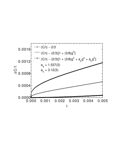
FIG. 4.: Difference $\Delta C/t$ between our Bethe ansatz electronic specific heat coefficient data and the exact coefficient 2/3 at $t=0$ (top data set), versus temperature $t$. Successive data sets show the influence of subtracting cumulative logarithmic correction terms.

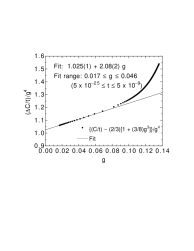
FIG. 5.: Plot showing the estimation of the coefficients of the $g^{4}$ and $g^{5}$ logarithmic correction terms in Eq. (13). The error bars on the data points are smaller than the symbols.

REFERENCES

- [1] H. A. Bethe, Z. Phys. 71, 205 (1931).
- [2] M. Takahashi, Prog. Theor. Phys. 46, 401 (1971); ibid. 50, 1519 (1973).
- [3] M. Suzuki and M. Inoue, Prog. Theor. Phys. 78, 787 (1987).
- [4] M. Takahashi, Phys. Rev. B 43, 5788 (1991); ibid. 44, 12 382 (1991).
- [5] S. Eggert, I. Affleck, and M. Takahashi, Phys. Rev. Lett. 73, 332 (1994).
- [6] J. C. Bonner and M. E. Fisher, Phys. Rev. 135, A640 (1964).
- [7] S. Lukyanov, Nucl. Phys. B 522, 533 (1998).
- [8] A. Klümper, Z. Phys. B 91, 507 (1993).
- [9] A. Klümper, Eur. Phys. J. B 5, 677 (1998).
- [10] I. Affleck, Phys. Rev. Lett. 56, 746 (1986).
- [11] I. Affleck, D. Gepner, H. J. Schulz, and T. Ziman, J. Phys. A 22, 511 (1989).
- [12] M. Karbach and K.-H. Mütter, J. Phys. A 28, 4469 (1995).
- [13] R. B. Griffiths, Phys. Rev. 133, A768 (1964); C. N. Yang and C. P. Yang, Phys. Rev. 150, 327 (1966).
- [14] D. C. Johnston et al., unpublished.