Fluctuating spin $g$-tensor in small metal grains

With the advance of nanoparticle technology, it has become possible to resolve individual energy levels for electrons in ultrasmall metal grains. Recent experiments addressed their Zeeman splitting under the application of a magnetic field $\vec{B}$ [1, 2, 3]. The splitting of a level $\varepsilon_{\mu}$ is described by a $g$-factor, $\delta\varepsilon_{\mu}=\pm\frac{1}{2}\mu_{B}gB_{z}$, where $\mu_{B}$ is the Bohr magneton. A free electron has $g=2$, but in small metal grains the effective $g$-factor may be reduced as a result of spin-orbit scattering [4]. In order to study this reduction, Salinas et al. [3] have doped Al grains (which do not have significant spin-orbit scattering) with Au (which has). For small concentrations of Au, the effective $g$-factor was seen to drop from 2 to around 0.7. Even lower values $g\sim 0.3$ were reported in experiments on Au grains [2].

For disordered systems with spin-orbit scattering, the splitting of a level $\varepsilon_{\mu}$ does not only depend on the magnitude of the magnetic field $\vec{B}$, but also on its direction. Hence, an analysis in terms of a “$g$-tensor” is more appropriate [5]. To be precise, the Zeeman field splits the Kramers’ doublet $\varepsilon_{\mu}\to\varepsilon_{\mu}\pm\delta\varepsilon_{\mu}$ with

$$\delta\varepsilon_{\mu}^{2}=(\mu_{B}/2)^{2}\vec{B}\cdot{\cal G_{\mu}}\cdot\vec{B},$$ (1)

where ${\cal G}_{\mu}$ is a $3\times 3$ tensor. In the absence of spin-orbit scattering, the tensor ${\cal G}_{\mu}$ is isotropic, $({\cal G_{\mu}})_{ij}=4\delta_{ij}$. The effect of spin-orbit scattering on ${\cal G}_{\mu}$ is threefold: It leads to a decrease of the typical magnitude of ${\cal G}_{\mu}$, it makes the tensor structure of ${\cal G}_{\mu}$ important (i.e., it introduces an anisotropic response to the magnetic field $\vec{B}$), and it causes ${\cal G}_{\mu}$ to be different for each level $\varepsilon_{\mu}$. Hence ${\cal G}_{\mu}$ becomes a fluctuating quantity, and it is important to know its statistical distribution. The latter problem was addressed in a recent paper by Matveev et al. [6], however without considering the tensor structure of ${\cal G}_{\mu}$. The anisotropy of the $g$-tensor is a measurable quantity and we here consider the distribution of the entire tensor ${\cal G}_{\mu}$. The distribution $P({\cal G}_{\mu})$ is defined with respect to an ensemble of small metal grains of roughly equal size. The same distribution applies to the fluctuations of ${\cal G}_{\mu}$ as a function of the level $\varepsilon_{\mu}$ in the same grain.

In general, ${\cal G}_{\mu}$ has a contribution ${\cal G}_{\mu}^{\rm spin}$ from the magnetic moment of electron spins, and a contribution ${\cal G}_{\mu}^{\rm orb}$ for the orbital angular moment of the state $|\psi_{\mu}\rangle$. In Ref. [6], the typical sizes of both contributions were estimated as ${\cal G}^{\rm spin}\sim\tau_{\rm so}\Delta$ and ${\cal G}^{\rm orb}\sim\ell/L$, where $\tau_{\rm so}$ is the mean spin-orbit scattering time, $L$ is the grain size, $\Delta\propto L^{-3}$ is the mean level spacing, and $\ell\ll L$ is the elastic mean free path. We restrict ourselves to the spin contribution ${\cal G}^{\rm spin}$, which should be dominant for small grain sizes [6], provided $\tau_{\rm so}$ does not depend on system size, as should be the case for the experiments of Ref. [3]. When orbital contributions are important, the anisotropy of ${\cal G}$ will be affected by the shape of the grain. In that case, our main conclusions apply only to a roughly spherical grain. As the typical magnitude of ${\cal G}$ (we drop the superscript “spin” and the subscript $\mu$ if there is no ambiguity) depends on the microscopic parameters $\tau_{\rm so}$ and $\Delta$, which are in most cases not known accurately, we choose to have the typical magnitude of ${\cal G}$ serve as an external parameter in our theory.

We first present our main results. With a suitable choice of the coordinate axes (“principal axes”), the tensor ${\cal G}$ can be diagonalized. Writing its eigenvalues as $g_{j}^{2}$ and denoting the components of the magnetic field along the principal axes by $B_{j}$, $j=1,2,3$, Eq. (1) takes a particularly simple form,

$$\delta\varepsilon_{\mu}^{2}=\frac{1}{4}\mu_{B}^{2}(g_{1}^{2}B_{1}^{2}+g_{2}^{2}B_{2}^{2}+g_{3}^{3}B_{3}^{2}).$$ (2)

We refer to the numbers $g_{1}$, $g_{2}$, and $g_{3}$ as principal $g$-factors. For a generic metal grain of a cubic material, rotational symmetry implies that, for a given level $\varepsilon_{\mu}$, the positioning of the principal axes is entirely random in space, as long as they are mutually orthogonal. Hence, it remains to study the distribution $P(g_{1},g_{2},g_{3})$ of the principal $g$-factors $g_{1}$, $g_{2}$, and $g_{3}$ for the level $\varepsilon_{\mu}$. Our main result is, that for sufficiently strong spin-orbit scattering, $P(g_{1},g_{2},g_{3})$ is given by the distribution

$$P(g_{1},g_{2},g_{3})\propto\prod_{i<j}|g_{i}^{2}-g_{j}^{2}|\prod_{i}e^{-3g_{i}^{2}/2\langle g^{2}\rangle},$$ (3)

where $g^{2}=\frac{1}{3}(g_{1}^{2}+g_{2}^{2}+g_{3}^{2})$ is the average of $(2\delta\varepsilon_{\mu}/\mu_{B}B)^{2}$ over all directions of $\vec{B}$ and $\langle g^{2}\rangle$ is its average over the ensemble of grains. In random matrix theory [7], this distribution is known as the Laguerre ensemble. Without loss of generality we may assume that $g_{1}^{2}\leq g_{2}^{2}\leq g_{3}^{2}$. Figure 1 shows the averages $\langle g_{j}^{2}\rangle$ and a realization of the principal $g$-factors $g_{1}$, $g_{2}$, and $g_{3}$ for a specific sample, as a function of a parameter $\lambda\sim(\tau_{\rm so}\Delta)^{-1/2}$ measuring the strength of the spin-orbit scattering. (A formal definition of $\lambda$ in a random-matrix model will be given below.) From the figure, one readily observes that, typically, the three principal $g$-factors differ by a factor $2$–$3$. This implies that, in spite of the average rotational symmetry of the grains, the response of a given level $\varepsilon_{\mu}$ to an applied magnetic field is highly anisotropic because of mesoscopic fluctuations. The mathematical origin of this effect is the “level repulsion” factor $|g_{i}^{2}-g_{j}^{2}|$ in the probability distribution (3), which signifies that, to a certain extent, ${\cal G}_{\mu}$ can be viewed a as a “random matrix”.

FIG. 1.: Average of the squares of principal $g$-factors versus spin-orbit scattering strength $\lambda$, obtained from numerical simulation of the random matrix model (Fluctuating spin $g$-tensor in small metal grains) with $N=100$. Inset: $g_{1}$, $g_{2}$, and $g_{3}$ for a specific realization. We have included the sign of $g_{1}$; see the discussion below Eq. (13).

Let us now turn to a more detailed discussion of our results. Without magnetic field, the Hamiltonian ${\cal H}$ of the grain is invariant under time-reversal, so that all eigenstates come in doublets $|\psi_{\mu}\rangle$ and $|{\cal T}\psi_{\mu}\rangle$, where ${\cal T}\psi=i\sigma_{2}\psi^{*}$ is the time-reversal operator. To study the splitting of the doublets by a magnetic field, we add a term $\mu_{B}\vec{B}\cdot\vec{\sigma}$ to ${\cal H}$, $\vec{\sigma}=(\sigma_{1},\sigma_{2},\sigma_{3})$ being the vector of Pauli matrices. From degenerate perturbation theory we find that a level $\varepsilon_{\mu}$ is split into $\varepsilon_{\mu}\pm\delta\varepsilon_{\mu}$, with $\delta\varepsilon_{\mu}$ of the form (1). For the real symmetric $3\times 3$ matrix ${\cal G}_{\mu}$ one has

$${\cal G}_{\mu}=G_{\mu}^{\rm T}G_{\mu},$$ (4)

where $G_{\mu}$ is a real $3\times 3$ matrix with elements

$$(G_{\mu})_{1j}+i(G_{\mu})_{2j} = -2\langle{\cal T}\psi_{\mu}|\sigma_{j}|\psi_{\mu}\rangle$$ (5)

$$(G_{\mu})_{3j} = 2\langle\psi_{\mu}|\sigma_{j}|\psi_{\mu}\rangle,$$ (6)

We use random-matrix theory (RMT) to compute the distribution of ${\cal G}_{\mu}$. In RMT, the microscopic Hamiltonian ${\cal H}$ is replaced by a $2N\times 2N$ random hermitian matrix $H$, where at the end of the calculation the limit $N\to\infty$ is taken. (The factor $2$ accounts for spin.) The wavefunction $\psi_{\mu}(\vec{r})$ is replaced by an $N$-component spinor eigenvector $\psi_{\mu n}$ of $H$, where $n$ is a vector index. To study the effect of spin-orbit scattering, we take $H$ of the form

$$H(\lambda)=S\otimes\openone_{2}+i{\lambda\over\sqrt{4N}}\sum_{j}A_{j}\otimes\sigma_{j},$$ (8)

where $S$ ($A_{j}$) is a real symmetric (antisymmetric) $N\times N$ matrix with the Gaussian distribution

$$P(S) \propto e^{-(\pi^{2}/4N\Delta^{2})\,{\rm tr}\,S^{\rm T}S},$$ (9)

$$P(A_{j}) \propto e^{-(\pi^{2}/4N\Delta^{2})\,{\rm tr}\,A_{j}^{\rm T}A_{j}},\ \ j=1,2,3.$$ (10)

The Hamiltonian $H(\lambda)$ is similar to the Pandey-Mehta Hamiltonian used to describe the effect of time-reversal symmetry breaking in a system of spinless particles [8]. In Eq. (9), $\Delta$ is the average spacing between the Kramers doublets near $\varepsilon=0$. The amount of spin-orbit scattering is measured by the parameter $\lambda\sim(\tau_{\rm so}\Delta)^{-1/2}$ [4]. The case $\lambda=0$ corresponds to the absence of spin-orbit scattering, when $H=S$ is a member of the Gaussian Orthogonal Ensemble (GOE) of random matrix theory. The case $\lambda=(4N)^{1/2}$ corresponds to the case of strong spin-orbit scattering, when $H$ is a member of the Gaussian Symplectic Ensemble (GSE). The ensemble of Hamiltonians $H(\lambda)$ corresponds to a crossover from the GOE to the GSE. Similar crossovers were studied previously in the literature, in particular for the cases GOE–GUE and GSE–GUE (GUE is Gaussian Unitary Ensemble) [8, 9, 10, 11, 12].

The distribution of the tensor ${\cal G}_{\mu}$ for an eigenvalue $\varepsilon_{\mu}$ of the matrix $H(\lambda)$ is related to the statistics of eigenvectors of $H(\lambda)$ in this crossover ensemble. To deal with the twofold degeneracy of the eigenvalue $\varepsilon_{\mu}$, we combine the two $N$-component spinor eigenvectors $\psi_{\mu}$ and ${\cal T}\psi_{\mu}$ into a single $N$-component vector of quaternions $\bar{\psi}=(\psi,{\cal T}\psi)$ [7, 13]. The quaternion vector $\bar{\psi}$ can be parameterized as,

$$\bar{\psi}=\sum_{k=0}^{3}\alpha_{k}u_{k}\otimes\phi_{k},$$ (11)

where the $u_{k}$ are quaternion numbers with $\mbox{tr}\,u_{k}^{\dagger}u_{l}=2\delta_{kl}$ (“quaternion phase factors”), the $\phi_{k}$ are $N$-component real orthonormal vectors, and the $\alpha_{k}$ are positive numbers such that $\sum_{k}\alpha_{k}^{2}=1$ ($k,l=0,1,2,3$). A eigenvector in the GOE corresponds to $\alpha_{0}=1$, $\alpha_{1}=\alpha_{2}=\alpha_{3}=0$, while an eigenvector in the GSE has typically $\alpha_{0}\approx\alpha_{1}\approx\alpha_{2}\approx\alpha_{3}\approx\frac{1}{2}$. A similar parameterization has been applied to the GOE–GUE crossover [9]. Orthogonal invariance of the distributions of $S$ and $A_{j}$, together with the freedom to choose the overall quaternion phase of $\bar{\psi}$, give a distribution of the $u_{k}$ and $\phi_{k}$ that is as random as possible, provided the above mentioned orthogonality constraints are obeyed. Hence, all nontrivial information about the eigenvector statistics is encoded in the numbers $\alpha_{k}$. Substitution of the parameterization (11) into Eq. (6) yields

$$g_{1} = 2(\alpha_{0}^{2}+\alpha_{1}^{2}-\alpha_{2}^{2}-\alpha_{3}^{2}),$$ (12)

$$g_{2} = 2(\alpha_{0}^{2}-\alpha_{1}^{2}+\alpha_{2}^{2}-\alpha_{3}^{2}),$$ (13)

$$g_{3} = 2(\alpha_{0}^{2}-\alpha_{1}^{2}-\alpha_{2}^{2}+\alpha_{3}^{2}).$$ (14)

While the squares $\alpha_{k}^{2}$ ($k=0,1,2,3$) are all positive, the principal $g$-factors as given by Eq. (13) can also be negative. Permutations of the $\alpha_{k}$ alter the signs of the individual $g_{j}$, but not of their product $g_{1}g_{2}g_{3}$. [The product $g_{1}g_{2}g_{3}=\det G$ also follows from Eq. (6); one verifies that it does not change when $|\psi\rangle$ is replaced by a linear combination of $|\psi\rangle$ and $|{\cal T}\psi\rangle$.] Without loss of generality, we may assume that $g_{1}^{2}\leq g_{2}^{2}\leq g_{3}^{2}$, and that $g_{2}$ and $g_{3}$ are positive. Then equation (13) provides the constraint $g_{2}+g_{3}\leq 2+g_{1}$, which poses a bound on the occurrence of negative values for the product $g_{1}g_{2}g_{3}$. We conclude that all information on the eigenvector statistics in the GOE–GSE crossover is encoded in the magnitudes of $g_{1}$, $g_{2}$, and $g_{3}$ and the sign of their product. Since for the level splitting $\delta\varepsilon_{\mu}(\vec{B})$ only the squares $g_{j}^{2}$ are of relevance, we disregard the sign of $g_{1}g_{2}g_{3}$ in the remainder of the paper. The sign of $g_{1}g_{2}g_{3}$ may be determined in principle, however, by a spin-resonance experiment [14].

In order to calculate the distribution $P(g_{1},g_{2},g_{3})$ one has, in principle, to carry out the same program as was done in Refs. [10, 11] for the GOE–GUE crossover. However, it turns out that in the present case the calculation is considerably more complicated. This can already be seen from the mere observation that the wavefunction statistics in the GOE–GSE crossover is governed by three variables $g_{1}$, $g_{2}$, and $g_{3}$, whereas in the case of the GOE–GUE crossover only one variable was needed [10, 11, 12]. In the field-theoretic language of Ref. [11], one has to use a nonlinear sigma model of $16\times 16$ supermatrices, instead of the usual $8\times 8$ for the GOE–GUE crossover [15]. Here we refrain from such a truly heroic enterprise. Instead we focus on the regimes of strong and weak spin-orbit coupling, and study the intermediate regime by means of numerical simulations of the model (Fluctuating spin $g$-tensor in small metal grains).

Before we address the case of strong spin-orbit scattering $\lambda\gg 1$ in the crossover Hamiltonian, we first consider the GSE, corresponding to $\lambda^{2}=4N$. In the GSE, the wavefunction $\psi$ is a vector of independently Gaussian distributed complex numbers. Then, one easily verifies that, for large $N$, the elements of the matrix $G$ of Eq. (6) are real random variables, independently distributed, with a Gaussian distribution of zero mean and variance $2/N$. Hence $G$ is a random real matrix with distribution

$$P(G)\propto\exp(-N{\rm tr}\,G^{\rm T}G/4).$$ (15)

The principal $g$-factors are the eigenvalues $g_{j}^{2}$ of the product ${\cal G}=G^{\rm T}G$. The distribution of the eigenvalues of such a matrix product is known in literature [16]. It is given by Eq. (3) with $\langle g^{2}\rangle=6/N$.

Let us now turn to the Hamiltonian $H(\lambda)$ for large $\lambda\gg 1$, but still $\lambda\ll N^{1/2}$. In that case, spin-rotation invariance is broken globally (so that a wavefunction as a whole does not have a well-defined spin), but not locally; on short length scales, the particle keeps a well-defined spin. We then argue that, in the random matrix language, one may think of the quaternion wavevector $\bar{\psi}$ as consisting of $\sim\lambda^{2}\gg 1$ components, each with a well-defined spin (or “quaternion phase”), but with uncorrelated spins for each component. The distribution of ${\cal G}$ is then given by the distribution for the GSE with $N$ replaced by a number $\sim\lambda^{2}$ [17]. We have found that the precise correspondence is $N\to 2\lambda^{2}$, by estimating the exponential term in the exact distribution, along the lines of Ref. [10, 17]. In order to verify this statement we have numerically generated random matrices of the form (Fluctuating spin $g$-tensor in small metal grains). The comparison with the GSE distribution with $N$ replaced by $2\lambda^{2}$ is excellent, see Fig. 2.

FIG. 2.: Distribution of the orientationally averaged $g$-factor $g^{2}=(g_{1}^{2}+g_{2}^{2}+g_{3}^{2})/3$ (upper left) and of the ratios $r_{12}=|g_{1}/g_{2}|$ (circles) and $r_{23}=|g_{2}/g_{3}|$ (squares, main figure). The solid curves are computed from the theory (17), the data points are numerical simulations of the random matrix model (Fluctuating spin $g$-tensor in small metal grains) with $N=200$ and $\lambda=7.7$. The slight discrepancy between theory and simulations for $r_{12}$ is a finite-$N$ effect; good agreement is obtained with the GSE distribution with $N=200$ (dotted curve). The lower inset shows $\langle g^{2}\rangle$ vs. $1/N$ for $\lambda=4.3$ (diamonds), $6.2$ (squares), and $8.1$ (open circles), together with the theoretical prediction $\langle g^{2}\rangle=3\lambda^{-2}$ for $N\to\infty$ (closed circles).

In order to further analyze $P({\cal G})$ for strong spin-orbit scattering, we introduce the orientationally averaged $g$-factor,

$$g^{2}=\frac{1}{3}(g_{1}^{2}+g_{2}^{2}+g_{3}^{2})=\left\langle{(2\delta\varepsilon_{\mu}/\mu_{B}|B|)^{2}}\right\rangle_{\Omega},$$ (16)

where the brackets $\langle\ldots\rangle_{\Omega}$ indicate an average over all directions of the magnetic field. Further, we introduce the ratios $r_{12}=|g_{1}/g_{2}|$ and $r_{23}=|g_{2}/g_{3}|$ to characterize the anisotropy of ${\cal G}$. Changing variables in Eq. (3), we find that $P(g,r_{12},r_{23})$ reads

$$P \propto {r_{23}^{3}(1-r_{23}^{2})(1-r_{23}^{2}r_{12}^{2})(1-r_{12}^{2})\over(1+r_{23}^{2}+r_{23}^{2}r_{12}^{2})^{9/2}}\,g^{8}e^{-9g^{2}/2\langle g^{2}\rangle}.\!$$ (17)

Note that the distribution of $r_{12}$ and $r_{23}$ does not depend on $\langle g^{2}\rangle$ (provided the spin-orbit scattering is sufficiently strong). The “$g$-factor” $g_{z}$ for a magnetic field in the $z$-direction (which is a random direction with respect to the principal axes) is given by $g_{z}=({\cal G}_{zz})^{1/2}$. Its distribution follows from Eq. (15) as $P(g_{z})\propto g_{z}^{2}\exp(-3g_{z}^{2}/2\langle g^{2}\rangle)$, in agreement with Ref. [6].

The case of weak spin-orbit scattering can be addressed by treating the terms proportional to $\lambda$ in Eq. (Fluctuating spin $g$-tensor in small metal grains) as a small perturbation. To second order in $\lambda$ we find,

$${\cal G}=4-{4\lambda^{2}}\sum_{\nu\neq\mu}a_{\mu\nu}^{\rm T}a_{\mu\nu}^{\vphantom{nosuperscript{\rm T}}}{1\over(\varepsilon_{\nu}-\varepsilon_{\mu})^{2}},$$ (18)

where $\Delta$ is the mean level spacing and $a_{\mu\nu}$ is an antisymmetric $3\times 3$ matrix proportional to the matrix elements of the perturbation in the eigenbasis $\{|\psi_{\nu}\rangle\}$ of $H(0)=S$, $(a_{\mu\nu})_{ij}=N^{-1/2}\langle\psi_{\mu}|A_{k}|\psi_{\nu}\rangle\varepsilon_{kij}$, where $\varepsilon_{kij}$ is the antisymmetric tensor. We first consider the change in the principal $g$-factors due to the matrix element $a_{\mu\nu}$ coupling the level $\varepsilon_{\mu}$ to a close neighboring level $\varepsilon_{\nu}$ where $\nu=\mu+1$ or $\mu-1$. (Level repulsion rules out the possibility that both levels $\varepsilon_{\mu\pm 1}$ are very close.) In view of the energy denominators in Eq. (18), we may expect that this contribution is dominant. Taking only the relevant matrix element $a_{\mu\nu}$ into account, we find

$$g_{3}=2,\ \ g_{1}=g_{2}=2-{\frac{1}{2}\lambda^{2}}{(\varepsilon_{\mu}-\varepsilon_{\nu})^{-2}}{\rm tr}\,a_{\mu\nu}^{\rm T}a_{\mu\nu}^{\vphantom{nosuperscript{\rm T}}},$$ (19)

where $\nu=\mu\pm 1$. Since the spacing distribution $P(|\varepsilon_{\mu}-\varepsilon_{\nu}|)\approx\pi\Delta^{-2}|\varepsilon_{\mu}-\varepsilon_{\nu}|$ for small $\varepsilon_{\mu}-\varepsilon_{\nu}$ [7], we find that the distribution $P(g)$ of both $g_{1}$ and $g_{2}$ has tails $P(g)=(3\lambda^{2}/2\pi)(2-g)^{-2}$ for $2-g\gg\lambda^{2}$. The main effect of contributions from the other energy levels in Eq. (18) is a reduction of $g_{3}$ below $2$, and a separation of $g_{1}$ and $g_{2}$. This is illustrated in Fig. 1. The three regimes of weak, intermediate, and strong spin-orbit scattering are compared in Fig. 3, using a numerical evaluation of the distributions of the three principal $g$-values.

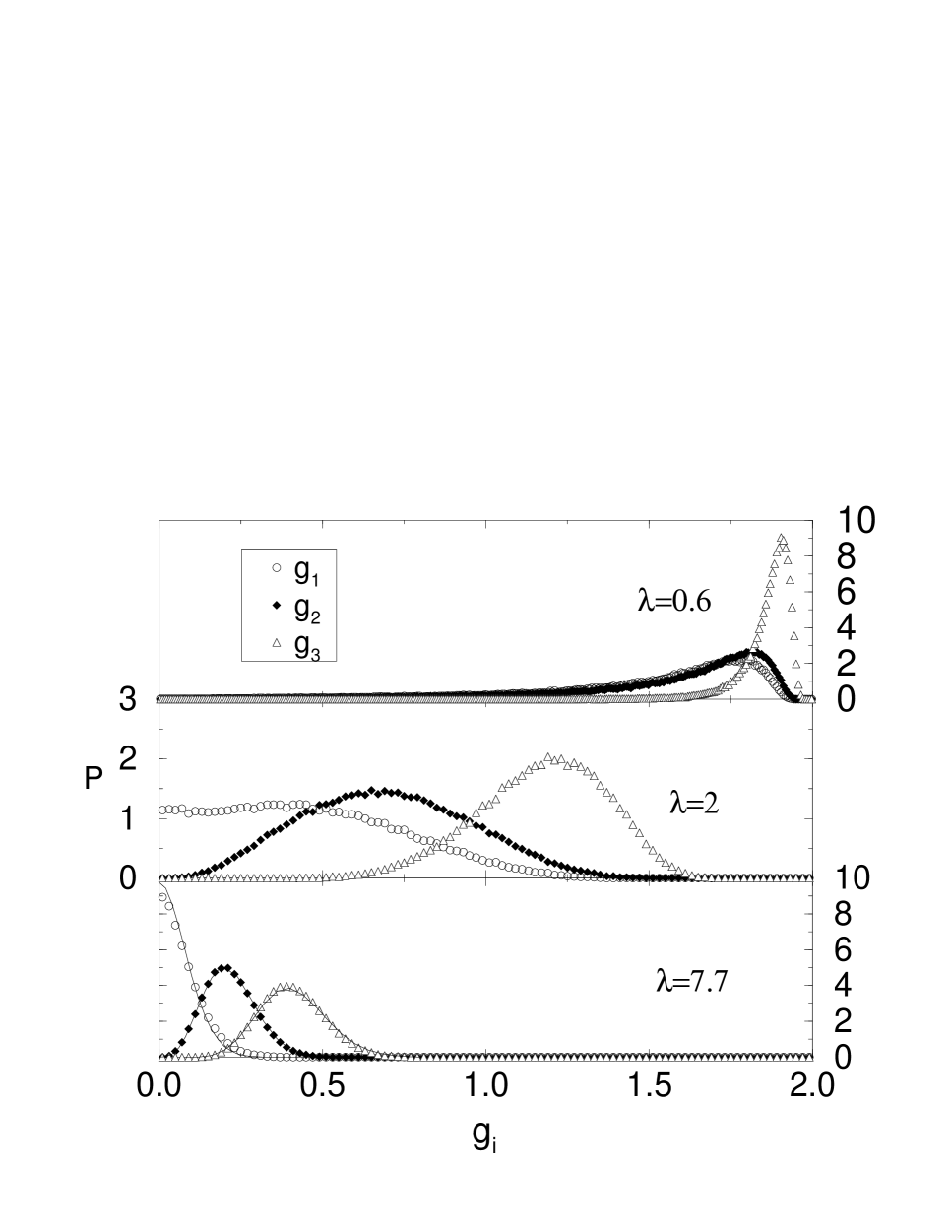
FIG. 3.: Distributions of the principal $g$-factors $g_{1}$, $g_{2}$, $g_{3}$ for $\lambda=0.6$, $2.0$, and $7.7$. The data points are obtained from numerical simulation of Eq. (Fluctuating spin $g$-tensor in small metal grains) with $N=100$.

We gratefully acknowledge discussions with T. A. Arias, D. Davidovic, K. M. Frahm, Y. Oreg, D. C. Ralph, and M. Tinkham. Upon completion of this project, we learned of Ref. [6], which contains some overlap with our work. This work was supported in part by the NSF through the Harvard MRSEC (grant DMR 98-09363), and by grant DMR 99-81283.

REFERENCES

[1] D. C. Ralph, C. T. Black, and M. Tinkham, Phys.
Rev. Lett. 74, 3241 (1995); ibid78, 4087 (1997);
[2] D. Davidovic and M. Tinkham, Phys. Rev. Lett.
83, 1644 (1999); cond-mat/9910396.
[3] D. G. Salinas, S. Guéron, D. C. Ralph, C. T.
Black, and M. Tinkham, Phys. Rev. B 60, 6137 (1999).
[4] W. P. Halperin, Rev. Mod. Phys. 58, 533
(1986).
[5] C. P. Slichter, Principles of Magnetic
Resonance (Springer, Berlin, 1980).
[6] K. A. Matveev, L. I. Glazman, and A. I. Larkin,
cond-mat/0001431.
[7]
M. L. Mehta, Random Matrices (Academic, New York, 1991).
[8]
A. Pandey and M. L. Mehta, Commun. Math. Phys. 87, 449 (1983).
[9]
J. B. French, V. K. B. Kota, A. Pandey, and S. Tomsovic,
Ann. Phys. (N. Y.) 181, 198 (1988).
[10]
H.-J. Sommers and S. Iida, Phys. Rev. E 49, 2513 (1994).
[11]
V. I. Fal’ko and K. B. Efetov, Phys. Rev. B 50, 11267 (1994);
Phys. Rev. Lett. 77, 912 (1996).
[12]
S. A. van Langen, P. W. Brouwer, and C. W. J. Beenakker,
Phys. Rev. E 55, 1 (1997).
[13]
A quaternion is a matrix of the form
where the are real numbers ().
[14] For example, if the principal axes of are
labeled , , and ,
and we apply a static field , then a
resonant AC field , with ,
will produce spin flips for but not for .
[15]
K. M. Frahm, private communication.
[16]
E. Brézin, S. Hikami, and A. Zee, Nucl. Phys. B 464, 411 (1996).
[17]
The same is true for the GOE–GUE crossover, where the relevant
quantity is the “phase-rigidity” . The distribution for large magnetic fields
equals in the GUE, with replaced by , where
is a crossover parameter analogous to , see Ref. [12].