[

Nature of the Spin Glass State

Abstract

The nature of the spin glass state is investigated by studying changes to the ground state when a weak perturbation is applied to the bulk of the system. We consider short range models in three and four dimensions and the infinite range Sherrington-Kirkpatrick (SK) and Viana-Bray models. Our results for the SK and Viana-Bray models agree with the replica symmetry breaking picture. The data for the short range models fit naturally a picture in which there are large scale excitations which cost a finite energy but whose surface has a fractal dimension, $d_{s}$, less than the space dimension $d$. We also discuss a possible crossover to other behavior at larger length scales than the sizes studied.

]

The nature of ordering in spin glasses below the transition temperature, $T_{c}$, remains a controversial issue. Two theories have been extensively discussed: the “droplet theory” proposed by Fisher and Huse[1] (see also Refs. [2, 3, 4]), and the replica symmetry breaking (RSB) theory of Parisi[5, 6, 7]. An important difference between these theories concerns the number of large-scale, low energy excitations. In the RSB theory, which follows the exact solution of the infinite range SK model, there are excitations which involve turning over a finite fraction of the spins and which cost only a finite energy even in the thermodynamic limit. Furthermore, the surface of these excitations is argued[8] to be space filling, i.e. the fractal dimension of their surface, $d_{s}$, is equal to the space dimension, $d$. By contrast, in the droplet theory, the lowest energy excitation which involves a given spin and which has linear spatial extent $L$ typically costs an energy of order $L^{\theta}$, where $\theta$ is a (positive) exponent. Hence, in the thermodynamic limit, excitations which flip a finite fraction of the spins cost an infinite energy. Also, the surface of these excitations is not space filling, i.e. $d_{s}<d$.

Recently we[9, 10, 11] investigated this issue by looking at how spin glass ground states in two and three dimensions change upon changing the boundary conditions. Extrapolating from the range of sizes studied to the thermodynamic limit, our results suggest that the low energy excitations have $d_{s}<d$. Similar results were found in two dimensions by Middleton[12]. In this paper, following a suggestion by Fisher[13], we apply a perturbation to the ground states in the bulk rather than at the surface. The motivation for this is two-fold: (i) We can apply the same method both to models with short range interactions and to infinite range models, like the SK model, and so can verify that the method is able to distinguish between the RSB picture, which is believed to apply to infinite range models, and some other picture which may apply to short range models. (ii) It is possible that there are other low energy excitations which are not excited by changing the boundary conditions[14, 15].

We consider the short-range Ising spin glass in three and four dimensions, and, in addition, the SK and Viana-Bray[16] models. The latter is infinite range but with a finite average coordination number $z$, and is expected to show RSB behavior. All these models have a finite transition temperature.

Our results for the SK and Viana-Bray models show clearly the validity of the RSB picture. However, for the short range models, our data is consistent with a picture suggested by Krzakala and Martin[19] where there are extensive excitations with finite energy, i.e. their energy varies as $L^{\theta^{\prime}}$ with $\theta^{\prime}=0$, but $d_{s}<d$. In three dimensions, this picture is difficult to differentiate from the droplet picture where the energy varies as $L^{\theta}$, because of the small value of $\theta$ ($\simeq 0.2$, obtained from the magnitude of the change of the ground state energy when the boundary conditions are changed from periodic to anti-periodic[17]). It is easier to distinguish the two pictures in 4-D, even though the range of $L$ is less, because $\theta$ is much larger[18] ($\simeq 0.7$).

The Hamiltonian is given by

$${\cal H}=-\sum_{\langle i,j\rangle}J_{ij}S_{i}S_{j},$$ (1)

where, for the short range case, the sites $i$ lie on a simple cubic lattice in dimension $d=3$ or 4 with $N=L^{d}$ sites ($L\leq 8$ in 3-D, $L\leq 5$ in 4-D), $S_{i}=\pm 1$, and the $J_{ij}$ are nearest-neighbor interactions chosen from a Gaussian distribution with zero mean and standard deviation unity. Periodic boundary conditions are applied. For the SK model there are interactions between all pairs chosen from a Gaussian distribution of width $1/\sqrt{N-1}$, where $N\leq 199$. For the Viana-Bray model each spin is connected with $z=6$ spins on average, chosen randomly, the width of the Gaussian distribution is unity, and the range of sizes is $N\leq 399$. To determine the ground state we use a hybrid genetic algorithm introduced by Pal[20], as discussed elsewhere[10].

Let $S_{i}^{(0)}$ be the spin configuration in the ground state for a given set of bonds. Having found $S_{i}^{(0)}$, we then add a perturbation to the Hamiltonian designed to increase the energy of the ground state relative to the other states, and so possibly induce a change in the ground state. This perturbation, which depends upon a positive parameter $\epsilon$, changes the interactions $J_{ij}$ by an amount proportional to $S_{i}^{(0)}S_{j}^{(0)}$, i.e.

$$\Delta{\cal H}(\epsilon)=\epsilon{1\over N_{b}}\sum_{\langle i,j\rangle}S_{i}^{(0)}S_{j}^{(0)}S_{i}S_{j},$$ (2)

where $N_{b}$ is the number of bonds in the Hamiltonian. The energy of the ground state will thus increase exactly by an amount $\Delta E^{(0)}=\epsilon.$ The energy of any other state, $\alpha$ say, will increase by the lesser amount $\Delta E^{(\alpha)}=\epsilon\ q_{l}^{(0,\alpha)},$ where $q_{l}^{(0,\alpha)}$ is the “link overlap” between the states “0” and $\alpha$, defined by

$$q_{l}^{(0,\alpha)}={1\over N_{b}}\sum_{\langle i,j\rangle}S_{i}^{(0)}S_{j}^{(0)}S_{i}^{(\alpha)}S_{j}^{(\alpha)},$$ (3)

in which the sum is over all the $N_{b}$ pairs where there are interactions. Note that the total energy of the states is changed by an amount of order unity.

The decrease in the energy difference between a low energy excited state and the ground state is given by

$$\delta E^{(\alpha)}=\Delta E^{(0)}-\Delta E^{(\alpha)}=\epsilon\ (1-q_{l}^{(0,\alpha)}).$$ (4)

If this exceeds the original difference in energy, $E^{(\alpha)}-E^{(0)}$, for at least one of the excited states, then the ground state will change due to the perturbation. We denote the new ground state spin configuration by $\tilde{S}_{i}^{(0)}$, and indicate by $q_{l}$ and $q$, with no indices, the link- and spin-overlap between the new and old ground states.

Next we discuss the expected behavior of $q$ and $q_{l}$ for the various models. For the SK model, it is easy to derive the trivial relation, $q_{l}=q^{2}$ (for large $N$). Since RSB theory is expected to be correct, there are some excited states which cost a finite energy and which have an overlap $q$ less than unity. According to Eq. (4), these have a finite probability of becoming the new ground state. Hence the average value of $q$ and $q_{l}$ over many samples, denoted by $[\cdots]_{\mathrm{av}}$, should tend to a constant less than unity in the thermodynamic limit. This behavior is shown in the inset of Fig. 1. For the Viana-Bray model, where there is no trivial connection between $q$ and $q_{l}$, we show in Fig. 1 data for $R=(1-[q_{l}]_{\mathrm{av}})/(1-[q]_{\mathrm{av}})$ for several values of $\epsilon$. This also appears to saturate. We plot this ratio rather than $[q]_{\mathrm{av}}$ or $[q_{l}]_{\mathrm{av}}$ for better comparison with the short range case below. For both models we took $\epsilon$ to be a multiple of the transition temperature (the mean field approximation to it, $T_{c}^{MF}=\sqrt{z}$, for the Viana-Bray model), so that a perturbation of comparable magnitude was applied in both cases.

FIG. 1.: Data for $R=(1-[q_{l}]_{\mathrm{av}})/(1-[q]_{\mathrm{av}})$ for the Viana-Bray model with coordination number $z=6$ for several values of $\epsilon$. The curvature is a strong indication that the data tends to a non-zero value for $N\to\infty$, as for the SK model. The best fits to $a+b/N^{c}$, shown by the lines, give $a=0.872\pm 0.005,0.883\pm 0.01$ and $0.84\pm 0.03$ for $\epsilon=\sqrt{6},\epsilon=\sqrt{6}/2$ and $\epsilon=\sqrt{6}/4$ respectively. Inset: $1-[q]_{\mathrm{av}}$ for the SK model with the strength of the perturbation given by $\epsilon=1$. Because $q_{l}=q^{2}$, the behavior of $[q_{l}]_{\mathrm{av}}$ is very similar. The data is clearly tending to a constant at large $N$. The solid line is the best fit and has $a=0.377\pm 0.004$.

FIG. 2.: A scaling plot of the data for $[q]_{\mathrm{av}}$ in 3-D according to Eq. (8). The data collapse is very good with $\mu=0.44$. The solid curve is a polynomial fit ($\chi^{2}=14.9$, $d.o.f.=13$), constrained to go through the origin, omitting the $L=3$ data. The dashed line is the linear term in the fit.

What do we expect for the short range models? In the RSB theory, $1-[q]_{av}$ and $1-[q_{l}]_{av}$ (and hence the ratio $R$) should saturate to a finite value for large $L$. To derive the prediction of the droplet theory, suppose that the energy to create an excitation of linear dimension, $l$, has a characteristic scale of $l^{\theta^{\prime}}$ (we use $\theta^{\prime}$ rather than $\theta$ to allow for the possibility that this exponent is different from the one found by changing the boundary conditions). Let us assume that large clusters ($l\approx L$) dominate and ask for the probability that a large cluster is excited. The energy gained from the perturbation is $\epsilon(1-q_{l})\sim\epsilon/L^{(d-d_{s})}$ since $1/L^{(d-d_{s})}$ is the fraction of the system containing the surface (i.e. the broken bonds) of the cluster. Generally this will not be able to overcome the $L^{\theta^{\prime}}$ energy cost to create the cluster. However, there is a distribution of cluster energies and if we make the plausible hypothesis that this distribution has a finite weight at the origin, then the probability that the cluster is excited is proportional to $1/L^{d-d_{s}+\theta^{\prime}}$. In other words

$$1-[q]_{\mathrm{av}}\sim\epsilon/L^{\mu}\ \ {\mathrm{w}here}\ \ \mu=\theta^{\prime}+d-d_{s}.$$ (5)

As discussed above, $1-q_{l}$ is of order $1/L^{(d-d_{s})}$ and so

$$1-[q_{l}]_{\mathrm{av}}\sim\epsilon/L^{\mu_{l}}\ \ {\mathrm{w}here}\ \ \mu_{l}=\theta^{\prime}+2(d-d_{s}).$$ (6)

Similar expressions have been derived by Drossel et al.[21] in another context. Eqs. (5) and (6) are expected to be valid only asymptotically in the limit $\epsilon\to 0$. In order to include data for a range of values of $\epsilon$ we note that the data is expected to scale as

$$1-[q]_{\mathrm{av}} = F_{q}(\epsilon/L^{\mu}),$$ (7)

$$1-[q_{l}]_{\mathrm{av}} = L^{-(d-d_{s})}F_{q_{l}}(\epsilon/L^{\mu}),$$ (8)

where the scaling functions $F_{q}(x)$ and $F_{q_{l}}(x)$ both vary linearly for small $x$. Note that the above discussion applies also to a picture in which $\theta^{\prime}=0$ and $d_{s}<d$.

FIG. 3.: A plot of $R=(1-[q_{l}]_{\mathrm{av}})/(1-[q]_{\mathrm{av}})$, the surface to volume ratio of the clusters, in 3D as a function of system size for different different values of $\epsilon$. For clarity the $\epsilon=\tau/2$ data is omitted. The dependence on $\epsilon$ is quite weak, and for each value of $\epsilon$ the data gives a good fit to a straight line with slope [equal to $-(d-d_{s})$] consistent with Eq. (9). The inset shows a scaling plot of the data according to Eq. (8) with the same value of $\mu$ as in Fig. 2. The solid curve is a polynomial fit ($\chi^{2}=26.0$, $d.o.f.=18$).

A scaling plot of our results for $1-[q]_{\mathrm{av}}$ in 3D is shown in Fig. 2. We consider a range of $\epsilon$ from $\sqrt{6}/4$ to $4\sqrt{6}$ (note that $T_{c}^{MF}=\sqrt{6}$) and find that the data collapse well onto the form expected in Eq. (8) with $\mu=0.44\pm 0.02.$

It is also convenient to plot the ratio $R$, which represents the surface to volume ratio of the excited clusters. This has a rather weak dependence on $\epsilon$ and, as shown in Fig. 3, the data for each of the values of $\epsilon$ fits well the power law behavior $L^{-(d-d_{s})}$, expected from Eqs. (5) and (6), with $d-d_{s}$ between 0.40 and 0.41 (the goodness of fit parameter, $Q$, is $0.07,0.03,0.85,0.23,0.10$, in order of increasing $\epsilon$). The inset to Fig. 3 shows that there are small deviations from the asymptotic behaviour, which can be accounted for by a scaling function with the same value of $\mu$ as in Fig. 2 and with

$$d-d_{s}=0.42\pm 0.02\ \ (3D).$$ (9)

From this value of $\mu$ and Eqs. (5) and (9) we find

$$\theta^{\prime}=0.02\pm 0.03\ \ (3D).$$ (10)

In order to test the RSB prediction, we tried fits of the form $R=a+b/L^{c}$, which give $a=0.28\pm 0.18,0.01\pm 0.14,0.04\pm 0.11$, and $-0.28\pm 0.18$ ($Q=0.08,0.01,0.72$, and 0.52) for $\epsilon/\tau=0.25,0.5,1$ and $2$. These are consistent with $a=0$ though a fairly small positive value, which would imply $d_{s}=d$, cannot be ruled out. For $\epsilon/\tau=4$ the fit gives a small positive value, $0.18\pm 0.07$ ($Q=0.79$), but this is likely too large a value of $\epsilon$ to be in the asymptotic regime for these sizes (see the inset of Fig. 3). The form $R=a+b/L+c/L^{2}$ also fits reasonably well the data and gives $a$ between 0.41 and 0.48 ($Q=0.16,0.03,0.82,0.80,0.16$). However, for both forms the data are very far from the asymptotic limit $R\sim a$ for the sizes considered, unlike for the Viana-Bray model (compare the main parts of Figs.  1 and  3). By contrast, the deviation from the asymptotic behavior $R\sim L^{-(d-d_{s})}$ is quite small (see the inset of Fig. 3).

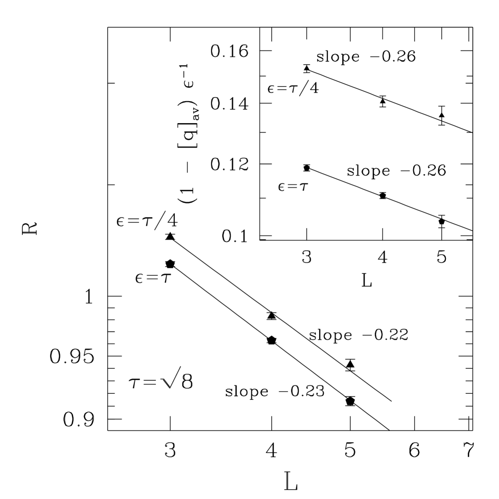
FIG. 4.: The main figure shows the ratio $R=(1-[q_{l}]_{\mathrm{av}})/(1-[q]_{\mathrm{av}})$ for different values of $\epsilon$ in 4-D. The inset shows corresponding data for $[q]_{\mathrm{av}}$.

In Fig. 4 we show analogous results in 4-D. The calculations were performed for two different values $\epsilon=\sqrt{8}/4$ and $\sqrt{8}$ ($=T_{c}^{MF}$). The exponents are essentially the same for these two values of the perturbation and the fits give $\mu=0.26\pm 0.04$, $d-d_{s}=0.23\pm 0.02$ , and so from Eq. (5) we get our main results for 4D:

$$\theta^{\prime}=0.03\pm 0.05,\quad d-d_{s}=0.23\pm 0.02\ \ (4D).$$ (11)

The data in Fig. 4 is consistent with the scaling form in Eq. (8) but the data for the two values of $\epsilon$ are too widely separated to demonstrate scaling.

Interestingly, our results in both 3-D and 4-D are consistent with $\theta^{\prime}=0$, and, within the error bars, (which are purely statistical) incompatible with the relation $\theta^{\prime}=\theta$, since $\theta\simeq 0.20$ in 3-D[17, 10] and $\theta\simeq 0.7$ in 4-D[18]. In 3-D, $\theta-\theta^{\prime}$ is small, but in 4-D this difference is larger and hence the conclusion that $\theta^{\prime}\neq\theta$ is stronger. However, the conclusion that $d-d_{s}>0$ is less strong in 4-D because our value for $d-d_{s}$ is quite small and the range of sizes is smaller than in 3-D.

It would be interesting, in future work, to study the nature of these excitations to see how they differ from the excitation of energy $L^{\theta}$ (with $\theta>0$) induced by boundary condition changes[10, 17, 18]. In particular, if their volume is space filling, one would expect a non-trivial order parameter distribution, $P(q)$, at finite temperatures.

To conclude, an interpretation of our results for short range models which is natural, in that it fits the data with a minimum number of parameters and with small corrections to scaling, is that there are large-scale low energy excitations which cost a finite energy, and whose surface has fractal dimension less than $d$. This picture differs from the one suggested by Houdayer and Martin[15], in which $d_{s}=d$. Furthermore, the results for short range models appear quite different from those of the mean-field like Viana-Bray model for samples with a similar coordination number and a similar number of spins. Other scenarios, such as the droplet theory (with $\theta^{\prime}=\theta\ (>0)$) or an RSB picture (where $\theta^{\prime}=0,d-d_{s}=0$), require larger corrections to scaling, but we cannot rule out the possibility of crossover to one of these behaviors at larger sizes.

We would like to thank D. S. Fisher for suggesting this line of enquiry, and for many stimulating comments. We also acknowledge useful discussions and correspondence with G. Parisi, E. Marinari, O. Martin, M. Mézard and J.-P. Bouchaud. We are grateful to D. A. Huse, M. A. Moore and A. J. Bray for suggesting the scaling plot in Fig. 2 and one of the referees for suggesting plotting the ratio $R$. This work was supported by the National Science Foundation under grant DMR 9713977. M.P. also is supported in part by a fellowship of Fondazione Angelo Della Riccia. The numerical calculations were supported by computer time from the National Partnership for Advanced Computational Infrastructure.

REFERENCES

- [1] D. S. Fisher and D. A. Huse, J. Phys. A. 20 L997 (1987); D. A. Huse and D. S. Fisher, J. Phys. A. 20 L1005 (1987); D. S. Fisher and D. A. Huse, Phys. Rev. B 38 386 (1988).
- [2] A. J. Bray and M. A. Moore, in Heidelberg Colloquium on Glassy Dynamics and Optimization, L. Van Hemmen and I. Morgenstern eds. (Springer-Verlag, Heidelberg, 1986).
- [3] W. L. McMillan, J. Phys. C 17 3179 (1984).
- [4] C. M. Newman and D. L. Stein, Phys. Rev. B 46, 973 (1992); Phys. Rev. Lett., 76 515 (1996); Phys. Rev. E 57 1356 (1998).
- [5] G. Parisi, Phys. Rev. Lett. 43, 1754 (1979); J. Phys. A 13, 1101, 1887, L115 (1980; Phys. Rev. Lett. 50, 1946 (1983).
- [6] M. Mézard, G. Parisi and M. A. Virasoro, Spin Glass Theory and Beyond (World Scientific, Singapore, 1987).
- [7] K. Binder and A. P. Young, Rev. Mod. Phys. 58 801 (1986).
- [8] E. Marinari, G. Parisi, F. Ricci-Tersenghi, J. Ruiz-Lorenzo and F. Zuliani, J. Stat. Phys. 98, 973 (2000).
- [9] M. Palassini and A. P. Young, Phys. Rev. B60, R9919, (1999).
- [10] M. Palassini and A. P. Young, Phys. Rev. Lett. 83, 5216 (1999).
- [11] M. Palassini and A. P. Young, cond-mat/9910278.
- [12] A. A. Middleton, Phys. Rev. Lett. 83, 1672 (1999).
- [13] D. S. Fisher, private communication.
- [14] N. Kawashima, J. Phys. Soc. Jpn. 69, 987 (2000).
- [15] J. Houdayer and O. C. Martin, Europhys. Lett. 49, 794 (2000).
- [16] L. Viana and A. J. Bray, J. Phys. C 18, 3037 (1985).
- [17] A. K. Hartmann, Phys. Rev. E 59, 84 (1999). A. J. Bray and M. A. Moore, J. Phys. C, 17, L463 (1984); W. L. McMillan, Phys. Rev. B 30, 476 (1984).
- [18] A. K. Hartmann, Phys. Rev. E 60, 5135 (1999). K. Hukushima, Phys. Rev. E 60, 3606 (1999).
- [19] F. Krzakala and O. C. Martin cond-mat/0002055.
- [20] K. F. Pal, Physica A 223, 283 (1996); K. F. Pal, Physica A 233, 60 (1996).
- [21] B. Drossel, H. Bokil, M. A. Moore and A. J. Bray, Eur. Phys. J. 13, 369 (2000).