Wetting-induced effective interaction potential between spherical particles

Abstract

Using a density functional based interface displacement model we determine the effective interaction potential between two spherical particles which are immersed in a homogeneous fluid such as the vapor phase of a one-component substance or the A-rich liquid phase of a binary liquid mixture composed of A and B particles. If this solvent is thermodynamically close to a first-order fluid-fluid phase transition, the spheres are covered with wetting films of the incipient bulk phase, i.e., the liquid phase or the B-rich liquid, respectively. Below a critical distance between the spheres their wetting films snap to a bridgelike configuration. We determine phase diagrams for this morphological transition and analyze its repercussions on the effective interaction potential. Our results are accessible to force microscopy and may be relevant to flocculation in colloidal suspensions.

I Introduction

In view of understanding a particular phenomenon in condensed matter, theory is supposed to identify the corresponding relevant degrees of freedom and to provide the effective interaction between them by, approximately, integrating out the remaining ones so that one is left with a manageable model. It is a major challenge to determine the effective interactions because that requires to calculate the partition function of the whole system under the constraint of a fixed configuration of the relevant degrees of freedom. The benefit for carrying out this constrained calculation, which in general is more difficult than the original full problem, is twofold. First, there is a gain in transparency by describing the system in terms of relevant degrees of freedom. Secondly, it is typically less risky to apply approximations for the partial trace because they only concern the less relevant degrees of freedom.

The determination of the phase behavior and of the structural properties of multi-component fluids represents a case study for this general approach. If the composing particles of the mixture are of comparable size and shape their degrees of freedom have to be treated on equal footing. The well developed machinery of liquid state theory [1] offers various techniques to cope with this problem. However, these techniques fail to yield reliable results if, e.g., one component is much larger than the others; in this case numerical simulations become inefficient and integral theories lose their accuracy. Colloidal suspensions are a paradigmatic case for such highly asymmetric solutions. For their description these difficulties can be overcome by resorting to the general scheme laid out at the beginning with the positions of the colloidal particles as the relevant degrees of freedom. Accordingly the degrees of freedom of the small solvent particles are to be integrated out for a fixed configuration of the colloidal particles which we assume to be smooth, monodisperse spheres. At sufficiently low concentrations of the suspended particles this leads to an effective pair potential between them. In many cases the effective potential resembles the bare one, i.e., the one in the absence of the solvent, but with modified, effective interaction parameters which depend on the thermodynamic variables of the system such as pressure and temperature.

The effective pair potential acquires additional new features if the solvent is enriched with particles of medium size such as, e.g., polymers. If the colloidal particles come close to each other the depletion zones around them, generated by the finite size of the medium particles, overlap leading to an entropically driven attraction of the colloidal particles [2, 3]. Correlation effects can modify the form and the range of these depletion forces considerably [4, 5]. These effective potentials have indeed turned out to be successful in describing the phase behavior of colloidal suspensions [6].

Qualitatively new aspects arise if the solvent particles exhibit a strong cooperative behavior of their own such as a phase transition which proliferates to the effective potential between the large particles. If the solvent undergoes a continuous phase transition, thermal Casimir forces between the large particles are induced due to the geometrical constraint they pose for the critical fluctuations [7, 8]. Such forces are long-ranged and have a strong influence on the phase behavior of the colloidal particles [9, 10]. If the solvent is thermodynamically close to a first-order phase transition, wetting phenomena [11] can occur at the surfaces of the dissolved particles (see Ref. [12] and references therein). If the bulk phase of the solvent is the vapor phase of a one-component fluid, the surfaces of the large spheres can be covered by a liquidlike wetting film. This situation corresponds to aerosol particles floating in a vapor. If the bulk phase of the solvent is the A-rich liquid phase of a binary liquid mixture composed of (small) A and B molecules, the dissolved colloidal particles can be coated by the B-rich liquid phase of the mixture. If the wet spheres approach each other, at a critical distance the two wetting films snap to a bridgelike structure. This morphological phase transition is expected to yield a nonanalytic form of the effective interaction potential between the large spheres. This nonanalyticity demonstrates that cooperative phenomena among those degrees of freedom which are integrated out can leave clearly visible fingerprints on the effective interaction between the remaining relevant degrees of freedom. The study of this kind of profileration is not only of theoretical interest in its own right but seems to play an important (albeit not exclusive [13]) role for the experimentally observed flocculation of colloidal particles dissolved in a binary liquid mixture close to its demixing transition into an A-rich and a B-rich liquid phase [14, 15, 16, 17, 18]. This observation has triggered numerous theoretical efforts devoted to various possible explanations of it. Since they are reviewed in Sec. I of Ref. [12] and more recently in Ref. [19] the interested reader is referred to there and we refrain from repeating this discussion here.

In our present analysis of this problem we apply density functional theory [20] which offers two advantages. First, this technique is particularly well suited to calculate, as required here, free energies under constraints. Secondly, it allows one to keep track of the basic molecular interaction potentials of the system. We focus our interest on thermodynamic states of the solvent which are sufficiently far away from its critical point so that the emerging liquid-vapor interfaces of the wetting films exhibit only a small width. Therefore we can apply the so-called sharp-kink approximation which considers only steplike variations of the solvent density distribution and thus leaves the interface position as the main statistical variable. This approximation has turned out to be surprisingly accurate for the description of wetting phenomena [21]. Our analysis extends and goes beyond previous efforts [22, 23] which are based on a similar interface displacement model grounded on a phenomenological ansatz. Whereas Refs. [22] and [23] are aimed at mapping out the phase diagram in terms of interaction parameters for the bridging transition mentioned above, we focus on the effective interaction potentials between the wet spheres, which are not presented in Refs. [22] and [23], and on their microscopic origin. Inter alia, this allows us to compare the effective interaction potential between the colloidal particles with the bare one, i.e., in the absence of the solvent, and thus to comment on the quantitative relevance of the solvent-mediated interaction. Moreover, we present the phase diagram of the system in terms of the thermodynamic variables temperature and chemical potential which is also not contained in Refs. [22] and [23].

In Sec. II we describe the implementation of a simple version of density functional theory for the present problem. For reasons of simplicity we confine our analysis to liquid-vapor coexistence of a one-component solvent; the generalization to a binary solvent is straightforward. In Sec. III we present some examples for the numerically calculated wetting film morphologies and discuss a phase diagram for the aforementioned morphological transition, and in Sec. IV we analyze the effective wetting-induced interaction potential between the spheres as a function of the distance between the spheres and the undersaturation. The experimental relevance of our model calculations is discussed in Sec. V and Sec. VI summarizes our main results. The Appendix contains some technical details.

II Density functional theory

A Model

We consider two identical, homogeneous, and smooth spherical particles of radius $R$ whose centers of mass are separated by a distance $D$ (see Fig. 1). They are immersed in a fluid of particles of number density $\rho({\mathbf{r}})$ which interact via a Lennard-Jones potential

$$\phi(r)=4\epsilon\left(\left(\frac{\sigma}{r}\right)^{12}-\left(\frac{\sigma}{r}\right)^{6}\right).$$ (1)

The system is symmetric with respect to a rotation around the axis which connects the centers of mass of the spheres (Fig. 1) and with respect to a reflection at a plane in the middle between the spheres that is perpendicular to the symmetry axis. Since we work in a grand canonical ensemble and the fluid particles are subject to the external potential exerted by the spheres, the equilibrium number density profile of the fluid particles exhibits these symmetries, too. Therefore we describe the system in cylindrical coordinates $(r_{\perp},\phi,z)$, with the $z$ axis being the symmetry axis of the system. The two centers of mass of the spheres are located at $(r=0,z=\pm D/2)$ such that the spheres occupy the volumes ${\mathcal{S}}_{\pm}=\{{\mathbf{r}}(r_{\perp},\phi,z)=(x,y,z)=(r_{\perp}\cos\phi,r_{\perp}\sin\phi,z)\in{\mathbb{R}}^{3}|\pm D/2-R\leq z\leq\pm D/2+R,\sqrt{r_{\perp}^{2}+(z\mp D/2)^{2}}\leq R\}$. The external potential exerted by both spheres on each individual fluid particle is

$$v_{tot}(r_{\perp},z;R)=v\left(\sqrt{r_{\perp}^{2}+(z-D/2)^{2}};R\right)+v\left(\sqrt{r_{\perp}^{2}+(z+D/2)^{2}};R\right)$$ (2)

where (see Eq. (A.4) in Ref. [12])

$$v(r;R) = \frac{9}{8}u_{9}\left(\frac{1}{r(r+R)^{8}}-\frac{1}{r(r-R)^{8}}\right)-u_{9}\left(\frac{1}{(r+R)^{9}}-\frac{1}{(r-R)^{9}}\right)$$ (4)

$$-\frac{3}{2}u_{3}\left(\frac{1}{r(r+R)^{2}}-\frac{1}{r(r-R)^{2}}\right)+u_{3}\left(\frac{1}{(r+R)^{3}}-\frac{1}{(r-R)^{3}}\right)$$

is the interaction potential between a single sphere of radius $R$ and a fluid particle at a distance $r>R$ from the center of mass of the sphere. In a continuum description, $v(r;R)$ follows from an integration of the Lennard-Jones potential

$$\phi_{sf}(r)=4\epsilon_{sf}\left(\left(\frac{\sigma_{sf}}{r}\right)^{12}-\left(\frac{\sigma_{sf}}{r}\right)^{6}\right)$$ (5)

between a molecule of the spherical substrate and a fluid particle. The subscript $sf$ denotes the parameters of the dispersion interaction between a particle in the fluid and a particle in the spheres. One has $u_{3}=\frac{2\pi}{3}\epsilon_{sf}\rho_{s}\sigma_{sf}^{6}$ and $u_{9}=\frac{4\pi}{45}\epsilon_{sf}\rho_{s}\sigma_{sf}^{12}$ where $\rho_{s}$ is the number density of the particles forming the spheres. (Many colloidal particles exhibit an even more complicated substrate potential because they are coated by a material different from their core so that they are no longer radially homogeneous as assumed for Eq. (4).)

Within our density functional approach the equilibrium particle number density distribution of the inhomogeneous fluid surrounding the spheres in a grand canonical ensemble minimizes the functional [20]

$$\Omega([\rho({\mathbf{r}})];T,\mu) = \int\limits_{{\mathcal{V}}_{f}}d^{3}r\Big{(}f_{HS}(\rho({\mathbf{r}}),T)+\big{(}v_{tot}({\mathbf{r}})-\mu\big{)}\rho({\mathbf{r}})\Big{)}$$ (7)

$$+\frac{1}{2}\int\limits_{{\mathcal{V}}_{f}}\int\limits_{{\mathcal{V}}_{f}}d^{3}r\,d^{3}r^{\prime}\,w(|{\mathbf{r}}-{\mathbf{r}}^{\prime}|)\rho({\mathbf{r}})\rho({\mathbf{r}}^{\prime}).$$

${\mathcal{V}}_{f}={\mathcal{V}}\setminus({\mathcal{S}}_{+}\cup{\mathcal{S}}_{-})$ is the volume accessible for the fluid particles, ${\mathcal{V}}$ is the total volume of the system; ${\mathcal{V}}\to{\mathbb{R}}^{3}$ in the thermodynamic limit. Equation (7) does not include the bare interaction potential $\Phi(D;R)$ (see, c.f., Sec. V) between the solid spheres, separated by vacuum, generated by the dispersion forces between the molecules forming the two spheres. $f_{HS}(\rho,T)$ is the free energy density of a hard-sphere fluid of number density $\rho$ at temperature $T$. In Eq. (7), the hard-sphere reference fluid is treated in local density approximation. We apply the Weeks-Chandler-Andersen procedure [24] to split up $\phi(r)$ into an attractive part $\phi_{att}(r)$ and a repulsive part $\phi_{rep}(r)$. The latter gives rise to an effective, temperature dependent hard-sphere diameter

$$d(T)=\int\limits_{0}^{2^{1/6}\sigma}dr\,\left(1-\exp\left(-\frac{\phi_{rep}(r)}{k_{B}T}\right)\right)$$ (8)

which is inserted into the Carnahan-Starling expression [25]

$$f_{HS}(\rho,T)=k_{B}T\rho\left(\ln(\rho\lambda^{3})-1+\frac{4\eta-3\eta^{2}}{(1-\eta)^{2}}\right)$$ (9)

for the free energy density $f_{HS}$ of the hard-sphere fluid, where $\eta=\frac{\pi}{6}\rho(d(T))^{3}$ is the dimensionless packing fraction and $\lambda$ is the thermal de Broglie wavelength. We approximate the attractive part of the interaction $\phi_{att}(r)$ by

$$w(r)=\frac{4w_{0}\sigma^{3}}{\pi^{2}}(r^{2}+\sigma^{2})^{-3}$$ (10)

with

$$w_{0}=\int_{{\mathbb{R}}^{3}}d^{3}r\,w(r)=\int_{{\mathbb{R}}^{3}}d^{3}r\,\phi_{att}(r)=-\frac{32}{9}\sqrt{2}\pi\epsilon\sigma^{3}$$ (11)

in order to simplify subsequent analytical calculations. The double integral in Eq. (7) takes into account this attractive interaction within mean-field approximation.

In the bulk the particle density $\rho_{\gamma}$ (where $\gamma=l,g$ denotes the liquid and vapor phase, respectively) is spatially constant, leading to (see Eq. (7))

$$\Omega_{b}(\rho_{\gamma},T,\mu)=f_{HS}(\rho_{\gamma},T)+\frac{1}{2}w_{0}\rho_{\gamma}^{2}-\mu\rho_{\gamma}$$ (12)

for the grand canonical free energy density of the bulk fluid. Minimization of $\Omega_{b}$ with respect to $\rho_{\gamma}$ yields the equilibrium densities. The line $\mu=\mu_{0}(T)$ of bulk liquid-vapor coexistence and the two bulk densities $\rho_{l}$ and $\rho_{g}$ at coexistence follow from

$$\left.\frac{\partial\Omega_{b}}{\partial\rho}\right|_{\rho=\rho_{g}}=\left.\frac{\partial\Omega_{b}}{\partial\rho}\right|_{\rho=\rho_{l}}=0\quad\mbox{and}\quad\Omega_{b}(\rho_{g})=\Omega_{b}(\rho_{l}).$$ (13)

For $\mu\neq\mu_{0}$, i.e., off coexistence, only the liquid or the vapor phase is stable. In this case the density of the metastable phase corresponds to the second local minimum of $\Omega_{b}$.

B General expressions for the contributions to the effective interaction potential

Henceforth we consider the case that the substrate is sufficiently attractive so that the liquid phase is preferentially adsorbed. Therefore, if in the bulk the vapor phase is stable ($\mu\leq\mu_{0}$), the fluid density is significantly increased in the vicinity of both spheres. In the spirit of the so-called sharp-kink approximation (see Sec. I and Ref. [21]) we assume that a thin film of constant density $\rho_{l}$ but with locally varying thickness is adsorbed at the surfaces of the spheres, separating the spheres from the bulk vapor phase of density $\rho_{g}$. This wetting film encapsulating both spheres is characterized by a function $h(z)$:

$$\rho({\mathbf{r}})=\rho(r_{\perp},\phi,z)=\Theta(r_{\perp}-(R+d_{s}))\bigg{(}\Theta(h(z)-r_{\perp})\rho_{l}+\Theta(r_{\perp}-h(z))\rho_{g}\bigg{)}$$ (14)

where $\Theta$ denotes the Heaviside step function. The length $d_{s}$ takes into account the excluded volume at the surfaces of the spheres which the centers of the fluid particles cannot penetrate due to repulsive forces. The profile $h(z)$ as given by Eq. (14) can describe both a configuration in which the wetting films surrounding each sphere are connected by a liquid bridge as well as the configuration in which both single spheres are surrounded by disjunct wetting layers. In the latter configuration there is a region around $z=0$ with $h(z)=0$.

Inserting $\rho(r_{\perp},\phi,z)$ from Eq. (14) into the functional $\Omega$ in Eq. (7) leads to a decomposition of $\Omega=\mbox{Vol}({\mathcal{V}}_{f})\Omega_{b}(\rho_{g})+\Omega_{S}$ into a bulk and subdominant contributions. The bulk contribution is $\mbox{Vol}({\mathcal{V}}_{f})\Omega_{b}(\rho_{g})$ (with $\Omega_{b}$ given by Eq. (12)) and corresponds to the vapor phase which is stable in the bulk. The subdominant contribution is

$$\Omega_{S}[h]=\Omega_{sl}+\Omega_{ex}[h]+\Omega_{ei}[h]+\Omega_{lg}[h]$$ (15)

where only $\Omega_{sl}$ is independent of $h(z)$ and all the other three contributions are functionals of $h(z)$. Since we have not found an indication for spontaneous symmetry breaking, in the following we discuss only symmetric configurations with $h(z)=h(-z)$.

$$\Omega_{ex}[h(z)]=\mbox{Vol}({\mathcal{L}})\Big{(}\Omega_{b}(\rho_{l})-\Omega_{b}(\rho_{g})\Big{)}$$ (16)

with

$$\mbox{Vol}({\mathcal{L}})=2\pi\int\limits_{0}^{L_{z}}dz\,h^{2}(z)-\frac{8\pi}{3}R^{3}$$ (17)

is an excess contribution which takes into account that the volume ${\mathcal{L}}={\mathcal{K}}\setminus({\mathcal{S}}_{-}\cup{\mathcal{S}}_{+})$ is filled with the metastable liquid instead of the vapor phase; ${\mathcal{K}}=\{{\mathbf{r}}(r_{\perp},\phi,z)\in{\mathbb{R}}^{3}|r_{\perp}\leq h(z)\}$ is the volume enclosed by the liquid-vapor interface. (The excluded volume due to $d_{s}$ enters into $\Omega_{sl}$ (see, c.f., Eq. (23)).) This free energy contribution $\Omega_{ex}$ vanishes at two-phase coexistence $\mu=\mu_{0}(T)$ (compare Eq. (13)). $2L_{z}$ is the extension of the total volume of the system ${\mathcal{V}}$ in $z$ direction; $L_{z}\to\infty$ in the thermodynamic limit and $h(z>z_{max})=0$ with $z_{max}\ll L_{z}$.

$$\Omega_{ei}[h(z)]=2\Delta\rho\int\limits_{{\mathcal{V}}_{-}\setminus{\mathcal{K}}_{-}}d^{3}r\,\Big{(}\rho_{l}(t({\mathbf{r}},{\mathcal{S}}_{-})+t({\mathbf{r}},{\mathcal{S}}_{+}))-v_{tot}({\mathbf{r}})\Big{)}$$ (18)

can be interpreted as the integrated effective interaction between the spheres and the liquid-vapor interface described by $h(z)$; $\Delta\rho=\rho_{l}-\rho_{g}$. ${\mathcal{V}}_{-}$ is that part of the volume ${\mathcal{V}}$ with $z<0$ (we note again that ${\mathcal{V}}_{-}\to{\mathbb{R}}_{-}^{3}$ in the thermodynamic limit which is always considered here), analogously ${\mathcal{K}}_{-}$ is the part of the set ${\mathcal{K}}$ with $z<0$. In Eq. (18) we have introduced the interaction potential

$$t({\mathbf{r}};{\mathcal{M}})=\int\limits_{{\mathcal{M}}}d^{3}r^{\prime}\,w(|{\mathbf{r}}-{\mathbf{r}}^{\prime}|)$$ (19)

between a fluid particle at ${\mathbf{r}}$ and a region ${\mathcal{M}}$ (with ${\mathbf{r}}\not\in{\mathcal{M}}$) homogeneously filled with the same fluid particles (analogous to the function $t(z)$ introduced in Refs. [11] and [21] in the case of a planar substrate). $v_{tot}$ is the total interaction potential between a fluid particle and both spheres (see Eq. (2)). Finally,

$$\Omega_{lg}[h(z)]=-(\Delta\rho)^{2}\int\limits_{{\mathcal{V}}_{-}\setminus{\mathcal{K}}_{-}}d^{3}r\,\Big{(}t({\mathbf{r}};{\mathcal{K}}_{-})+t({\mathbf{r}};{\mathcal{K}}_{+})\Big{)}$$ (20)

is the free energy contribution from the free liquid-gas interface. It is a nonlocal functional of $h(z)$ in contrast to $\Omega_{ex}$ and $\Omega_{ei}$ whose dependence on $h(z)$ enters only via the integration volume ${\mathcal{K}}_{-}$. The local approximation thereof, which is provided by the gradient expansion of Eq. (20), is

$$\Omega_{lg}^{loc}=4\pi\sigma_{lg}^{(p)}\int\limits_{0}^{L_{z}}dz\,h(z)\,\sqrt{1+\left(\frac{dh}{dz}\right)^{2}}.$$ (21)

In Eq. (21)

$$\sigma_{lg}^{(p)}=-\frac{1}{2}(\Delta\rho)^{2}\int\limits_{0}^{\infty}dz\,\int\limits_{z}^{\infty}dz^{\prime}\int\limits_{{\mathbb{R}}^{2}}d^{2}r_{\parallel}w\left(\sqrt{r_{\parallel}^{2}+z^{\prime 2}}\right)$$ (22)

is the interfacial tension of a planar, free liquid-vapor interface in sharp-kink approximation. We note that, strictly speaking, the surface tension of a curved liquid-vapor interface depends on the local radius of curvature (see Fig. 2 in Ref. [12] and the references therein concerning the Tolman length). This curvature dependence is omitted in the local model presented here. However, for spheres of radius $R\geq 20\sigma$ as considered henceforth the curvature correction is less than $1\%$. Similar arguments hold for the deviation of the actual liquidlike density in the wetting film from the bulk value $\rho_{l}$.

For our choice of interaction potentials (Eq. (1) and (5)) a tedious calculation leads to explicit expressions for the contributions $\Omega_{ei}$ and $\Omega_{lg}$ which are given in the Appendix. The remaining contribution

$$\Omega_{sl}=-\rho_{l}\int\limits_{{\mathcal{V}}_{-}\setminus{\mathcal{S}}_{-}}d^{3}r\,\Big{(}\rho_{l}(t({\mathbf{r}},{\mathcal{S}}_{-})+t({\mathbf{r}},{\mathcal{S}}_{+}))-2v_{tot}({\mathbf{r}})\Big{)}-\Omega_{b}(\rho_{l})\frac{8\pi}{3}((R+d_{s})^{3}-R^{3}),$$ (23)

which is independent of $h(z)$, is the sphere-liquid interfacial free energy corresponding to the interface between the spheres and the liquid phase. The last term in Eq. (23) takes into account the excluded volumes at the surfaces of the spheres. In the limit of large separations $D$ one has

$$\Omega_{sl}(D\to\infty)-2\Omega_{sl}^{(1)}\sim D^{-6}$$ (24)

with the sphere-liquid interfacial free energy $\Omega_{sl}^{(1)}$ of a single sphere immersed in the liquid phase. The leading power law $\sim D^{-6}$ in Eq. (24) can be inferred from the following consideration: if present, the second sphere displaces a spherical volume from the homogeneous liquid phase so that the free energy of the interaction of the first sphere with the bulk liquid is reduced by the interaction free energy of that sphere with the displaced spherical liquid volume. This latter interaction decays as $D^{-6}$ for large separations $D$, at which the dispersion interaction between two spherical objects resembles the dispersion interaction between two pointlike particles. (Here, as before, we have not yet taken into account the bare interaction potential $\Phi(D;R)$ between the two solid spheres; but see, c.f., Sec. V.)

Up to the bulk contribution the grand canonical potential of the system is the minimum of $\Omega_{S}[h(z)]$ with respect to the profile $h(z)$:

$$\Omega_{S}=\Omega_{S}(D;R)=\min_{\{h(z)\}}(\Omega[h(z)]).$$ (25)

Thus the equilibrium interface morphology $h(z)$ minimizes $\Omega_{S}[h(z)]$ which includes the contributions $\Omega_{ex}[h(z)]$, $\Omega_{ei}[h(z)]$, $\Omega_{lg}[h(z)]$, and $\Omega_{sl}$. The functional used in Refs. [22] and [23] (Eq. (1) in both references) is, albeit formulated in another coordinate system and using a more phenomenological ansatz for the basic interaction potentials, essentially identical with the sum $(\Omega_{lg}^{loc}+\Omega_{ex}+\Omega_{ei})[h(z)]$. However, this model description does neither incorporate the bare dispersion interaction of the two spheres (c.f., Sec. V) nor the free energy contribution $\Omega_{sl}$ which describes the sphere-liquid interfacial free energy. We emphasize that the consideration of the contribution $\Omega_{sl}$ – which does not depend on $h(z)$ – is not essential for the determination of the equilibrium wetting film morphology and hence it is not relevant for the thermodynamic phase diagram of thin-thick and bridging transitions (Fig. 2 in Ref. [23]) for a fixed separation $D$ between the spheres. But the term $\Omega_{sl}$ is crucial to the shape of the effective, wetting-induced interaction potential between the spheres, i.e., its dependence on $D$ (see Eq. (24)).

III Morphology of the wetting layers

A Interface profiles

The actual wetting layer morphology $h(z)$ follows from numerical minimization of the functional $\Omega_{S}[h(z)]$ (Eq. (15)) for a given temperature $T$ and undersaturation $\Delta\mu=\mu_{0}(T)-\mu$, with the contributions $\Omega_{ex}$ (Eq. (16)), $\Omega_{ei}$ (Eq. (18)), $\Omega_{sl}$ (Eq. (23)), and $\Omega_{lg}$ (Eq. (20) within the nonlocal and Eq. (21) for the local theory). Within a range of parameters $(T,\Delta\mu)$ the numerical minimization yields two different solutions for $h(z)$, one with a liquid bridge and one without, depending on the initial function $h(z)$ used in the iteration scheme for the minimization. For small separations $a\ll 2R$ only the solution which exhibits a liquid bridge is stable whereas for large separations $a\gg 2R$ only the solution without bridge minimizes $\Omega_{S}$. For large distances $D$ the minimization consistently yields twice the result known for a single individual sphere enclosed by a wetting film (compare Ref. [12]). This observation amounts to a useful check of the numerical procedure.

As a first example, in Fig. 2 we present the numerical results for a wetting layer enclosing two spheres of radius $R=20\sigma$. For our particular choice of interaction parameters, at coexistence $\Delta\mu=0$ the wetting film on each of the single spheres alone exhibits a first-order thin-thick transition (which is the remnant of the first-order wetting transition on the corresponding planar substrate, see Fig. 8(a) in Ref. [12]) at $T_{tt}^{*}=k_{B}T/\epsilon\approx 1.271$ (which corresponds to $T_{tt}/T_{c}\approx 0.9$ where $T_{c}$ is the critical temperature of gas-liquid coexistence in the bulk). The planar substrate, i.e., a single sphere in the limit $R\to\infty$, exhibits a genuine first-order wetting transition (with the film thickness jumping to a macroscopic value) at $T_{w}^{*}\approx 1.053$ ($T_{w}/T_{c}\approx 0.75$, $T_{tt}/T_{w}\approx 1.21$). Figure 2(a) depicts a typical solution with a bridge, here for a separation $a=D-2R=10\sigma$ ($D=50\sigma$) and the thermodynamic parameters $T^{*}=1.3>T_{tt}^{*}$ and $\Delta\mu=0$, i.e., at liquid-vapor coexistence. The solution without a bridge for the same choice of parameters is shown in Fig. 2(b). The latter solution has a higher free energy than the former one. Therefore the solution with bridge is thermodynamically stable whereas the solution without bridge is metastable. For the solution without a bridge the distortion of the liquidlike layer around one sphere due to the presence of the other sphere is not visible. Finally, Fig. 2(c) displays the wetting film morphology for the stable state with bridge at the temperature $T^{*}=1.2$, i.e., below the thin-thick transition temperature $T_{tt}^{*}$. (We note that the thin-thick transition temperature $T_{tt}$ for each sphere is slightly shifted by the presence of the second sphere. However, as already pointed out in Ref. [23], this effect is negligibly small.) In any case, the difference between the nonlocal and the local theory is very small. This latter result is in accordance with the findings for the comparison between the nonlocal and the local description of the three-phase contact line on a homogeneous substrate and of the wetting layer morphology on a chemically structured substrate (compare Ref. [26]). For this reason, henceforth we only consider the local theory.

Figure 3 shows another pertinent example. Here we study the wetting layer morphology for two larger spheres of radius $R=50\sigma$ as a function of the undersaturation $\Delta\mu$ along the isotherm $T^{*}=1.2$. The interaction potential parameters are the same as for the previous first example and the separation of the surfaces $a$ is $20\sigma$ ($D=120\sigma$). At coexistence each single sphere exhibits a first-order thin-thick transition at $T_{tt}^{*}\approx 1.191$ (i.e., $T_{tt}/T_{c}\approx 0.84$ and $T_{tt}/T_{w}\approx 1.13$). In analogy to the prewetting line on a homogeneous substrate there is a line of thin-thick transitions $(T,\Delta\mu_{tt}(T))$ which intersects the liquid-vapor coexistence line at $(T=T_{tt},\Delta\mu=0)$ (compare with, c.f., Fig. 4 and Fig. 8(a) in Ref. [12]). At the temperature $T^{*}=1.2>T_{tt}^{*}$ considered here the thin-thick transition occurs at $\Delta\mu_{tt}^{*}=\Delta\mu_{tt}/\epsilon\approx 0.0103$. Upon reducing the undersaturation along the isotherm, starting at, e.g., $\Delta\mu^{*}=0.05$, first the configuration with thin films and without bridge is stable (Fig. 3(a)). For $\Delta\mu\leq\Delta\mu_{bt}$ (bridging transition) with $\Delta\mu_{bt}^{*}\approx 0.0235>\Delta\mu_{tt}^{*}(T)$ the solution with bridge becomes stable, but the layers enclosing the spheres still remain thin (Fig. 3(b)). Upon further reduction of $\Delta\mu$, at $\Delta\mu_{tt}(T)$ the second transition from a solution with bridge and thin films to a solution with bridge and thick films (Fig. 3(c)) takes place. (As before, concerning the value of $T_{tt}^{*}$ at coexistence, also the value $\Delta\mu_{tt}^{*}(T)$ is practically unchanged by the presence of the second sphere – even for the bridge configuration.) We note that for this choice of parameters and in the case of a solution with bridge and thin films (Fig. 3(b)) the profile $h(z)$ exhibits six turning points instead of only two as for the case of a solution with bridge and thick films (Fig. 3(c)). This rich curvature behavior is caused by the details of the effective interaction potential between the spherical substrate surfaces and the liquid-vapor interface (see Sec. 2.3 in Ref. [12]), similar to the curvature behavior of the liquid-vapor interface when it meets a homogeneous, planar substrate forming a three-phase contact line (compare Ref. [26]). These features may also occur for a bridge configuration with thin films at coexistence and $T<T_{tt}$.

B Phase diagram

The example presented in the previous paragraph shows that besides the gas-liquid coexistence curve $\Delta\mu=0$ the $T$-$\Delta\mu$ phase diagram of the system contains two distinct lines of first-order phase transitions: a line of thin-thick transitions $(T,\Delta\mu_{tt}(T))$ on the single spheres (which is the remnant of the line of prewetting transitions on the corresponding flat substrate and which is, as stated above, practically unshifted by the presence of the second sphere) and a second, independent line of bridging transitions $(T,\Delta\mu_{bt}(T))$. If one crosses the latter along an isotherm $T=T_{0}$ approaching coexistence $(T_{0},\Delta\mu\to 0)$, at $\Delta\mu=\Delta\mu_{bt}(T_{0})$ a transition from the configuration without bridge $(\Delta\mu>\Delta\mu_{bt}(T_{0}))$ to a configuration with bridge $(\Delta\mu<\Delta\mu_{bt}(T_{0}))$ occurs. The derivative $\partial\Omega_{S}/\partial\Delta\mu$ is discontinuous at $\Delta\mu_{bt}$, indicating that the bridging transition is first order. Figure 4 shows the $T$-$\Delta\mu$ phase diagram for the two spheres with $R=20\sigma$ for $D=50\sigma$ ($a=10\sigma$). The line of thin-thick transitions intersects the liquid-vapor coexistence line at $T_{tt}^{*}\approx 1.271$ with a finite, negative slope (compare Fig. 8(a) in Ref. [12]). It extends into the vapor phase region ($\Delta\mu>0$) of the phase diagram and ends at a critical point. The line of bridging transitions intersects the coexistence line also with a finite, negative slope. On the other end, within our sharp-kink interface model, it happens to be cut off at that metastability line in the phase diagram at which the second minimum of the bulk free energy at high fluid density (Eq. (12)) ceases to exist so that for larger undersaturations the liquid phase is not even metastable. Within a more sophisticated approach, e.g., by seeking the full minimal density distributions of Eq. (7), the line of bridging transitions is expected to end in a critical point, too. (Concerning the effect of fluctuations on these mean field predictions see the following paragraph.) The line of bridging transitions is entirely located in the region where the liquidlike films on the spheres are thin. Moreover, the effect of the presence of the liquid bridge on the line of thin-thick transitions is negligibly small. In Fig. 4 the relative location of the bridging transition line and the thin-thick transition line corresponds to our specific choice of the interaction potential parameters as well as the chosen size of and distance between the spheres. Changing these parameters will lead to shifts of these lines and, possibly, to different topologies of the phase diagram. Here we refrain from exhaustingly presenting all possibilities which can occur according to Refs. [22] and [23].

Since the liquid volume enclosed by the interface $h(z)$ is quasi-zerodimensional, fluctuation effects destroy the sharp first-order phase transition (see Refs. [27] and [28]). In Sec. 4 of Ref. [12] it has been extensively discussed how finite size effects smear out the thin-thick transition such that the thickness increases sharply but continuously within a range $\delta\mu$ around $\Delta\mu_{tt}(T)$; these results apply analogously to the present case. Using similar approximations we obtain a range $\delta\mu$ between $\delta\mu^{*}\approx 0.004$ for $T^{*}=1.16$ and $\delta\mu^{*}\approx 0.02$ for $T^{*}=1.26$ over which the bridging transitions shown in Fig. 4 are smeared out around $\Delta\mu_{bt}(T)$. Thus close to $\Delta\mu=0$ the quasi-first-order thin-thick transitions are clearly visible. However, for larger values of $\Delta\mu$ they become progressively smeared out such that their critical points predicted by mean field theory are erased by fluctuations.

IV Effective film-induced interaction potential

A Shape of the effective potential, metastability, and asymptotic behavior

In the following we change our point of view: we vary the distance $D$ between the centers of mass of the spheres instead of the thermodynamic parameters $T$ and $\Delta\mu$. Figure 5 shows the grand canonical potential $\Omega_{S}$ corresponding to the wetting layer morphologies for the case $R=20\sigma$ and $T^{*}=1.2$ (Fig. 2(c)) as a function of the separation $a=D-2R$ for several values of $\Delta\mu$. $\Omega_{S}$ is the minimum of $\Omega_{S}[h(z)]$ (Eq. (15)) for the given set of parameters $T$, $\Delta\mu$, and $D=2R+a$. For each value of $\Delta\mu$ there are two branches of the free energy, one corresponding to the solution without bridge, which for the case $R=20\sigma$ considered here exists only for $a\gtrsim 0.15R$, and the other corresponding to the solution with bridge which exists up to $a\approx 0.65R$ and $a\approx 0.6R$ for $\Delta\mu^{*}=0$ and $\Delta\mu^{*}=0.01$, respectively. At a certain value $D=D_{bt}$ or, equivalently, $a=a_{bt}$, which are functions of $\Delta\mu$, a first-order phase transition occurs with discontinuous derivative $\partial\Omega_{S}/\partial D$ between the solutions with and without bridge. The main effect of increasing the undersaturation $\Delta\mu$ is that the free-energy curves are rigidly shifted upwards. This shift is approximately proportional to $\Delta\mu$ and larger in the case of the solution with bridge, resulting in the dependence of $D_{bt}$ on $\Delta\mu$. The values of $\Omega_{S}$ shown in Fig. 5 are obtained within the local theory. The nonlocal theory yields the same functional dependence $\Omega_{S}(D)$ but with a slight and rigid shift of the free-energy curves, relative to the results of the local theory, of the order of $0.1\%$ and of the same sign and size for both the solutions with and without bridge. Finite-size effects again destroy the sharp first-order bridging transition; we obtain a range $\delta D\sim 0.1\sigma$ (corresponging to $\delta D\sim 0.005R$) over which the bridging transitions shown in Fig. 5 are smeared out.

The thermodynamic states which are located on the metastable branches of the free energy curves survive during an average lifetime $\tau\approx\tau_{0}\exp(\Delta\Omega_{S}/k_{B}T)$ where $\Delta\Omega_{S}$ is the height of the energy barrier that separates the metastable from the stable branch and $\tau_{0}$ is a characteristic microscopic time scale for the dynamics associated with the transition from a metastable to a stable wetting layer configuration. The energy barrier is highest in the vicinity of the bridging transition and vanishes near the ends of the metastable branches. An estimation of the energy barrier height yields, e.g., $\Delta\Omega_{S}\approx 75\epsilon$ for $\Delta\mu=0$ and $D=50\sigma$ ($a=0.5R$), and with $k_{B}T\sim\epsilon$ it follows that $\exp(\Delta\Omega_{S}/k_{B}T)\sim 10^{32}$, i.e., the metastable unbridged state for $a=0.5R$ near the bridging transition remains stable practically forever. However, at, e.g., $a=0.2R$ one has $\exp(\Delta\Omega_{S}/k_{B}T)\sim 10^{11}$ so that with $\tau_{0}\sim 1$ps$\dots 1$ns one may observe a decay of the metastable states near the ends of the metastable branches within seconds or minutes. Thus the change of the morphology of the wetting films is expected to exhibit pronounced hysteresis effects as function of $D$.

Obviously, in the limit of large separation $D\to\infty$ (in which only the configuration without a bridge is stable) the grand canonical potential $\Omega_{S}(D)$ approaches the limiting value $2\Omega_{S}^{(1)}$ corresponding to the free energy of two individual spheres, each surrounded by a wetting layer. It is convenient to separate this constant contribution $2\Omega_{S}^{(1)}$ from the grand canonical potential $\Omega_{S}$ of the system and thus to define an excess free energy $\Omega_{E}(D)=\Omega_{S}(D)-2\Omega_{S}^{(1)}$ which contains all contributions from the wetting-layer induced interaction between the two spheres. In the limit $D\to\infty$, i.e., in the absence of a liquid bridge, this excess free energy $\Omega_{E}(D)$ decays as $D^{-6}$ (see Eq. (24) and, c.f., Sec. V). We note that for the example shown in Fig. 5 the coefficient of this leading order is positive, i.e., the effective potential in the absence of a liquid bridge is repulsive. This is owed to the choice $T<T_{tt}$ for this example: the spheres disfavor the adsorption of thick liquid films and the presence of the second sphere with its surrounding liquidlike layer leads to an additional cost in free energy which diminishes for increasing $D$. For the choice $T>T_{tt}$, i.e., if the spheres favor the adsorption of liquid (e.g., for $T^{*}=1.3$ as in Figs. 2(a) and (b)) the coefficient of $D^{-6}$ is negative and the effective interaction is attractive. However, in the presence of a liquid bridge, i.e., for sufficiently small values of $D$, the effective potential shows the same qualitative behavior as in Fig. 5 also for the case of thick wetting layers ($T^{*}=1.3>T_{tt}^{*}$) as well as for the larger spheres ($R=50\sigma$) with thin or thick films.

B Effective interaction potential for large spheres

In this subsection we consider the limiting case that the sphere radius $R$ is much larger than the diameter $\sigma$ of the solvent particles and that the separations $a$ between the surfaces of the spheres are proportional to $R$: $R\gg\sigma$, $\sigma\ll a\approx R$. For such large separations as compared to $\sigma$ the contributions $\Omega_{sl}$ (Eq. (23)), $\Omega_{ei}$ (Eq. (18)), and $\Phi$ (c.f., Eq. (31)) become vanishingly small relative to the contributions $\Omega_{lg}$ (Eq. (20)) and $\Omega_{ex}$ (Eq. (16)). For the case described above $\Omega_{lg}$ and $\Omega_{ex}$ scale proportional to the surface area of the spheres, i.e., $\sim R^{2}$, whereas for $a/\sigma\to\infty$, $R/\sigma\to\infty$, $a/R$ finite, $\Phi(D;R)$ remains finite $\sim\epsilon_{ss}\sigma_{ss}^{6}\rho_{s}^{2}$ with a proportionality constant of the order $1$. Analogously, in the same limit $\Omega_{ei}-2\Omega_{ei}^{(1)}$ (Eq. (18)) and $\Omega_{sl}-2\Omega_{sl}^{(1)}$ (Eq. (23)) are determined by finite terms $\sim\Delta\rho\rho_{l}\epsilon\sigma^{6}$ and $\sim\Delta\rho\rho_{s}\epsilon_{sf}\sigma_{sf}^{6}$ and of terms $\sim\rho_{l}^{2}\epsilon\sigma^{6}$ and $\sim\rho_{l}\rho_{s}\epsilon_{sf}\sigma_{sf}^{6}$, respectively, each with a proportionality constant of the order $1$. Therefore measured in units of $8\pi R^{2}$ the unbridged branch of $\Omega_{E}$ in Fig. 5(b) vanishes in the limit $R\to\infty$. Moreover, on this scale the excluded volume at small $a$ disappears from the figure, too, because $d_{s}/R\to 0$.

Fig. 6 shows the excess effective interaction potential $\Omega_{E}$ in the limit of large spheres for the case $\Delta\mu=0$, i.e., at two-phase coexistence in the solvent. In this limit and for $\Delta\mu=0$, $\Omega_{lg}$ is the only relevant contribution to $\Omega_{S}$ because $\Omega_{ex}(\Delta\mu=0)=0$. Accordingly, in this case the bridging transition is determined by the equality of the surface areas of the liquid-vapor interfaces for the unbridged and bridged configuration. From this condition and from dimensional analysis it follows that for large spheres $D_{bt}(\Delta\mu=0)$ is determined by the equation

$$8\pi(R+l_{0})^{2}\sigma_{lg}^{(p)}=8\pi(R+l_{0})^{2}\sigma_{lg}^{(p)}f\left(\frac{D_{bt}}{R+l_{0}}\right)$$ (26)

where $f$ is, for dimensional reasons, a universal function of $D/(R+l_{0})$ alone which describes the surface area of the bridged configuration; $l_{0}$ is the equilibrium wetting layer thickness on a single sphere. Since the line of bridging transitions lies below the line of thin-thick transitions, $l_{0}$ remains microscopicly small at the bridging transition (Fig. 4). Therefore one has

$$D_{bt}(\Delta\mu=0)=\lambda(R+l_{0})$$ (27)

with a universal number

$$\lambda\approx 2.32$$ (28)

determined by $f(\lambda)=1$ (compare Fig. 6). If one applies this reasoning to Fig. 5 one finds $\lambda\approx 2.39$. Therefore even for $R=20\sigma$ this macroscopic approximation leads to a surprisingly small error of only $3\%$ for $D_{bt}(\Delta\mu=0)$. Accordingly, in Fig. 5 the full curves corresponding to $\Delta\mu=0$ closely resemble the ones in Fig. 6 describing the case of large spheres. The only differences appear for small separations $a$ where the bridged branch linearly extends down to its minimum value $\Omega_{E}/(8\pi(R/\sigma)^{2})\approx-0.0227\epsilon$ at $a/R=0$ (Fig. 6). Only in this range of separations the effect of the contributions $\Omega_{ei}$ and $\Omega_{sl}$ becomes significant, leading to the deeper minimum visible in Fig. 5. Thus for $\Delta\mu=0$ and large $R$ the dependence of the effective interaction potential on $R$ for the bridged configuration is captured by the indicated rescaling of the axes in Fig. 5(b). However, our numerical analysis shows that the smallness of the deviations between the macroscopic description valid for $R\gg\sigma$ and the actual results for $R=20\sigma$ is somewhat fortuitous. Whereas the dependence of $D_{bt}(\Delta\mu=0)$ on $R$ is indeed weak, the shape of the potential (for $\Delta\mu=0$) reduces to that shown in Fig. 6 only for $R$ larger than several hundred $\sigma$ and, surprisingly, for $R$ up to $20\dots 30\sigma$ with the deviations being maximal for $R\approx 100\sigma$.

Off coexistence $\Delta\Omega_{b}=\Omega_{b}(\rho_{l})-\Omega_{b}(\rho_{g})\approx\Delta\mu\Delta\rho$ is positive so that Eq. (26) has to be augmented correspondingly:

$$8\pi(R+l_{0})^{2}+\frac{8\pi\Delta\Omega_{b}}{3\sigma_{lg}^{(p)}}\left((R+l_{0})^{3}-R^{3}\right)={\mathcal{A}}+\frac{\Delta\Omega_{b}}{\sigma_{lg}^{(p)}}\mbox{Vol}({\mathcal{L}})$$ (29)

where ${\mathcal{A}}$ and $\mbox{Vol}({\mathcal{L}})$ (Eq. (17)) are the area of the liquid-vapor interface and the volume of the liquid, respectively, for the bridged configuration. They are obtained by inserting into Eqs. (21) and (17) that profile $h(z)$ which solves the differential equation determining the minimum of $\Omega_{lg}[h]+\Omega_{ex}[h]$ together with the appropriate boundary conditions. By splitting off a factor $(R+l_{0})^{2}$ from ${\mathcal{A}}$ and $(R+l_{0})^{3}$ from $\mbox{Vol}({\mathcal{L}})$ dimensional analysis shows that up to terms $\sim l_{0}/R$ the critical distance for the bridging transition is given by a universal scaling function $\Lambda$:

$$D_{bt}(\Delta\mu)=\Lambda\left(\frac{\Delta\rho\Delta\mu R}{\sigma_{lg}^{(p)}}\right)R$$ (30)

with $\Lambda(0)=\lambda$. Thus off coexistence the critical bridging transition depends, apart from an explicit factor $R$, on $R$ and $\Delta\mu$ via the scaling variable $\Delta\rho\Delta\mu R/\sigma_{lg}^{(p)}$. This property is shared by the whole bridged branch of the effective interaction potential. Thus increasing $R$ for fixed undersaturation $\Delta\mu$ has the same effect as increasing $\Delta\mu$ for fixed $R$. From Fig. 5(b), in which the unbridged branch will disappear in the limit $R\gg\sigma$, one infers that the range and the depth of $\Omega_{E}$ decrease for increasing $R$ at fixed undersaturation $\Delta\mu$. The behavior of $D_{bt}$ and of the bridged branch of the effective interaction potential off coexistence and for $R\to\infty$ is determined by the behavior of the scaling function $\Lambda(x)$ in the limit $x\to\infty$. Our numerical data indicate that $\Lambda(x\to\infty)<2$ so that due to the geometric constraint $D\geq 2R$ there is no bridging transition and the bridged branch of the effective potential vanishes for any value of $\Delta\mu$ in the limit $R\to\infty$. The cost in free energy due to the excess contribution $\Omega_{ex}$ suppresses the formation of a liquidlike bridge in the case of macroscopicly large spheres. In turn, this means that for any finite value of $\Delta\mu$ there is a large but finite critical radius $R_{c}$ for which the critical separation $a_{bt}$ for the bridging transition attains the value $a_{bt}=0$, such that for $R>R_{c}$ there is no bridging transition. The determination of $R_{c}$ requires to analyze the full dependence of $\Lambda$ on the scaling variable $x$. This, however, implies such a large numerical effort that it is beyond the scope of the present paper.

V Discussion

A Total interaction potential

The bare dispersion interaction between the two spheres is not included in Eq. (7). According to Hamaker [29] this contribution is given by

$$\Phi(D;R)=-\frac{A_{ss}}{12}\left(\frac{4R^{2}}{(D-2R)(D+2R)}+\frac{4R^{2}}{D^{2}}+2\ln\left(\frac{(D-2R)(D+2R)}{D^{2}}\right)\right)$$ (31)

as the dispersion interaction between two identical spheres of radius $R$ at center-of-mass distance $D$. In the limit $a/R\ll 1$, where $a=D-2R$ (see Fig. 1(a)) is the smallest separation between the surfaces of the spheres, Eq. (31) reduces to

$$\Phi(D=2R+a;R\gg a)\approx-\frac{A_{ss}}{12}\,\frac{R}{a}$$ (32)

which corresponds to the Derjaguin approximation whereas $\Phi(D\gg R;R)=-16A_{ss}R^{6}/(9D^{6})$. Thus except for the $D$-independent bulk contribution $\mbox{Vol}({\mathcal{V}}_{f})\Omega_{b}(\rho_{g})$ the total grand canonical potential of the system is

$$\Omega_{tot}(D;R)=\Omega_{S}(D;R)+\Phi(D;R)$$ (33)

where $\Omega_{S}(D;R)$ is given by the minimum value $\min_{\{h(z)\}}(\Omega_{S}[h(z)])$ for given $D$ and $R$ (Eqs. (15) and (25)); in analogy to $\Omega_{E}$ we define the excess total free energy $\Omega_{E,tot}=\Omega_{tot}-2\Omega_{S}^{(1)}$. $A_{ss}$ is the Hamaker constant appertaining to the bare dispersion interaction between the particles in the spheres. In the case of pairwise additivity of the molecular interactions and in the absence of retardation effects one has $A_{ss}=4\pi^{2}\epsilon_{ss}\sigma_{ss}^{6}\rho_{s}^{2}$ if the interaction potential between two individual molecules in the spheres is given by a Lennard-Jones potential (Eq. (5)) with the parameters $\epsilon_{ss}$ and $\sigma_{ss}$. Typically $A_{ss}$ is of the order of $10^{-19}$J or, equivalently, $10\dots 100\epsilon$. If the vacuum between the spheres is replaced by a medium of condensed matter the interaction between the spheres is screened [30]. In our present model this medium is the bulk vapor phase modified by the presence of the liquidlike films adsorbed on the spheres and the screening effect is described microscopicly by the functional $\Omega[\rho({\mathbf{r}})]$.

In Refs. [31] and [32] this additional screening effect, due to spherical shells of adsorbed, homogeneous layers surrounding spherical particles, on the dispersion interaction between the latter immersed in another homogeneous medium has been calculated macroscopicly. Beyond molecular scales these results should closely correspond to the configuration without liquid bridge discussed herein because the deviation of the spherical shape of one wetting layer due to the presence of the second sphere is very small. Indeed, the interaction energy calculated in Refs. [31] and [32] is practically the same as the sum of the $D$-dependent contributions in $\Omega_{ei}$ (Eq. (18)) and $\Omega_{sl}$ (Eq. (23)) for the configurations without bridge – for these configurations $\Omega_{lg}$ and $\Omega_{ex}$ do not contribute to the dependence of $\Omega_{S}$ on $D$ – and the direct dispersion interaction $\Phi(D;R)$. In Ref. [31] the total dispersion interaction is shown to be always attractive if the Hamaker constants $A_{ij}$ corresponding to the interaction between any two media $i$ and $j$ are chosen such that $A_{ij}=\sqrt{A_{ii}\,A_{jj}}$. Although the effective interaction induced by the wetting layers shown in Figs. 5(b) and 7 for the configuration without bridge is repulsive, we note that the sum $\Omega_{tot}$ of this interaction and of the bare dispersion potential $\Phi(D;R)$ is also attractive if we choose the Hamaker constant in Eq. (31) accordingly, i.e., $A_{ss}=A_{sf}^{2}/A$ (Fig. 7). Therefore our results are consistent with those obtained in Ref. [31]. Since only effective interactions between finite volumes enter into the total excess interaction potential $\Omega_{E,tot}$ and these effective interactions decay as $D^{-6}$ in the limit of large separations $D$, the same holds for $\Omega_{E,tot}$.

Figure 5 shows that as soon as the wetting films snap to a liquidlike bridge, whether it is stable or metastable, there is an attractive wetting-layer-induced force $-\partial\Omega_{E}/\partial D$ that pulls the spheres together. From Fig. 5 one can infer that this attractive force is of the order of $40\epsilon/\sigma$ in the range between $a\approx 4\sigma$ (i.e., $0.2R$ for $R=20\sigma$ discussed in this figure) and $a\approx 10\sigma$ ($0.5R$) where the effective potential varies almost linearly. At the small separation $a_{min}\approx 2.5\sigma$ the effective potential $\Omega_{E}$ induced by the bridgelike wetting layer is minimal and the wetting-induced force is zero. Finally, at smaller separations the interaction is repulsive leading to a stabilization of the spheres at $D=D_{min}=2R+a_{min}$. Within the range $a\ll R$ the bare, direct dispersion interaction between the spheres (Eqs. (31) and (32)) gives rise to a force $F_{bare}(a)\approx-A_{ss}R/12a^{2}$. The estimate $A_{ss}\approx 4\pi^{2}\epsilon_{sf}^{2}\sigma_{sf}^{12}\rho_{s}^{2}/\epsilon\sigma^{6}\sim 400\epsilon$ for the case of pairwise additive interactions without retardation follows from the ansatz $A_{sf}=\sqrt{A\,A_{ss}}$, so that the bare dispersion force in our example with $R=20\sigma$ is $F_{bare}(a)\approx-670\epsilon\sigma/a^{2}$. Therefore in the range where the bridge-induced force is almost constant ($4\sigma\lesssim a\lesssim 10\sigma$) the direct, bare dispersion force decays from approximately $-40\epsilon/\sigma$ (which is of the same order of magnitude as the bridge-induced force) to approximately $-6\epsilon/\sigma$, whereas for smaller separations it becomes the dominant force.

B Relevance for force microscopy

Our model calculations can be tested experimentally by force microscopy. This can be done by suitably fixing one sphere in the fluid and by attaching the second one to the tip of a force microscope. Alternatively, both spheres can be positioned by optical tweezers and the force law can be inferred by monitoring optically their dynamics after switching off the tweezers. At separations between the spheres which are comparable with the diameter $\sigma$ of the solvent particles the actual effective interaction potential will exhibit an additional oscillatory contribution due to packing effects which decays exponentially on the scale $\sigma$ [33]. In order to obtain these oscillations one would have to resort to density functional theories which are more sophisticated than the one in Eq. (7). This, in turn, would make it much more difficult to obtain the bridgelike configuration, to map out the complete phase diagram, and to obtain results for large spheres. According to Subsec. IV B, for $R\gg\sigma$ and at two-phase coexistence $\Delta\mu=0$ the bridging transition occurs at distances $a$ which are proportional to $R$. In this case, due to $R\gg\sigma$, the effective interaction potential will be practically unaffected by this oscillatory contribution for the vast portion $\sigma\ll a\ll a_{bt}$ of the range of the effective interaction potential.

C Relevance for charge stabilized colloidal suspensions

Whereas the kinds of experiments considered in the previous subsection are focused on two individual spherical particles, we discussed in the Introduction that the effective interaction potential enters into the collective behavior of colloidal suspensions such that the bridging transition may trigger flocculation. If colloidal suspensions would be governed by dispersion forces alone, most of them would flocculate even in the absence of the wetting-induced forces discussed here because the dispersion forces generate the so-called primary minimum in the effective interaction potential close to contact. Since this minimum is much deeper than $k_{B}T$ the colloidal particles would simply stick together permanently. This effect, which is undesired for many applications, can be avoided by endowing the particles with electrical charges which adds a screened Coulomb repulsion between the charged particles. As a result, such charge stabilized colloidal suspensions are characterized by effective interaction potentials in which a substantial energy barrier separates the aforementioned primary minimum from a second, much more shallow minimum at larger distances. Since this potential barrier is typically large compared with $k_{B}T$ the phase behavior of the colloidal particles is practically independent of the primary minimum formed by the dispersion forces and determined by the shape of the potential outside the barrier. As demonstrated by Figs. 5 and 7 the range of the wetting-induced forces is about $0.55R$, in good agreement with $D_{bt}\approx 2.32(R+l_{0})$ (see Eqs. (27) and (28)). On the other hand the position (and height) of the aforementioned energy barrier depends sensitively on the size of the total charge on the spheres, the amount of salt in the solvent, and the dispersion forces and can be varied over a wide range. With a high salt concentration the barrier position can be as small as a few tens of nm. Thus under such circumstances the wetting-induced interaction potentials would be relevant even for colloidal particles whose radii are only a few tens of nm.

D Relevance for stericly stabilized colloidal suspensions

There is another class of colloidal suspensions for which the wetting-induced forces can be of practical importance. By coating the colloidal particles with polymers and by matching the refractive indices of the colloidal particles and the bulk fluid (in our case study the vapor phase or, more realisticly in the present context, the A-rich liquid phase of a binary liquid mixture acting as the solvent) the colloidal particles behave effectively like hard spheres (see, e.g., Refs. [34] and [35]). Through this index matching the sum of the bare interaction potential $\Phi(D;R)$ and the effective interaction potential $\Omega_{sg}$, which would arise if the spheres were immersed in the homogeneous and unperturbed bulk solvent, vanishes. Within our model $\Omega_{sg}$ is given by the expression in Eq. (23) with $\rho_{l}$ replaced by $\rho_{g}$, which is the density of the bulk phase. Since the index matching works for the bulk phase, it does not work for the wetting phase. As a consequence the wetting-induced forces appear against a background effective potential of hard spheres. Therefore for this class of colloidal suspensions the wetting phenomena discussed here are expected to have a pronounced effect on their phase behavior. Within our model, for index-matched suspensions the total effective interaction potential is given by

$$\Omega_{tot,im}(D;R)=\Omega_{tot}(D;R)-(\Phi(D;R)+\Omega_{sg}(D;R))=\Omega_{S}(D;R)-\Omega_{sg}(D;R)$$ (34)

and in analogy to $\Omega_{E}$ and $\Omega_{E,tot}$ we define

$$\Omega_{E,im}(D;R)=\Omega_{tot,im}(D;R)-2\Omega_{im}^{(1)}(R)$$ (35)

with $\Omega_{E,im}(D\to\infty;R)=0$ for the unbridged solutions. Figure 8 displays $\Omega_{tot,im}$ and $\Omega_{E,im}$ as function of $a=D-2R$ for the same system as in Figs. 5 and 7. $\Omega_{sg}$ is about $30\%$ smaller than $\Omega_{S}$ for the unbridged solution and also approaches its asymptote $2\Omega_{sg}^{(1)}$ from above. As before (see the discussion of Fig. 7 above), the resulting total effective interaction between spheres in an index-matched bulk fluid for the state with liquid bridge is still attractive and of the same order of magnitude as the bare dispersion interaction between the spheres, i.e., in the absence of the solvent.

VI Summary

We have obtained the following main results:

1. Based on microscopic interaction potentials and within a simple version of density functional theory (Eqs. (7)–(11)) we have calculated the grand canonical potential of a system of two spheres immersed in a bulk fluid phase (Fig. 1). The microscopic interactions are chosen such that the spheres prefer the adsorption of a second fluid phase which is thermodynamically close to the bulk fluid phase. Accordingly, a single sphere immersed in the fluid is covered by a homogeneous wetting layer of this second phase of thickness $l_{0}$. These thin wetting layers covering the spheres lead to an effective wetting-induced interaction potential $\Omega_{S}(D)$ between the spheres. We have systematically determined the dependence of $\Omega_{S}$ on the distance $D$ between the spheres in terms of the morphology $h(z)$ of the wetting film enclosing the spheres (Eqs. (15)–(23)). We find that the shape of the effective interaction potential $\Omega_{S}(D)$ depends, inter alia, on the effective interaction of two spheres immersed in the homogeneous wetting phase (Eq. (23)). This contribution, which is independent of $h(z)$, is not incorporated in previous phenomenological models for this system [22, 23].

2. The equilibrium interfacial profiles of the wetting layers are determined numerically by minimizing the free energy functional $\Omega_{S}[h(z)]$ in Eqs. (15)–(23). We have calculated the rich structure of these equilibrium profiles (Fig. 3) for spheres of radii $R=20\sigma$ (Fig. 2) and $R=50\sigma$ (Fig. 3) where $\sigma$ denotes the diameter of the solvent particles. As function of distance $D$, temperature $T$, and undersaturation $\Delta\mu$ the system undergoes a first-order “bridging transition” between the two configurations shown in Fig. 1. For a fixed distance $D$ we have mapped out the phase diagram of bridging transitions in the $T$-$\Delta\mu$ plane (Fig. 4). It turns out that the bridging transition differs from and to a large extent is independent of the thin-thick transition of the wetting layer on each single sphere which is a remnant of the prewetting transition on the corresponding flat substrate. Thus one has to distinguish between the prewetting line for a first-order wetting transition on a planar substrate, the thin-thick transition line for wetting on a single sphere, and the bridging transition line for two spheres (Fig. 4). At two-phase coexistence $\Delta\mu=0$ and for $R\gg\sigma$ the bridging transition is determined by the equality of the surface areas of the interfaces in the bridged and the unbridged configuration, leading to a universal ratio $D_{bt}(\Delta\mu=0)/(R+l_{0})\approx 2.32$ for the critical distance $D_{bt}(\Delta\mu=0)$ of the bridging transition at coexistence (Fig. 6 and Subsec. IV B). Off coexistence $D_{bt}(\Delta\mu,R)$ is described by a universal scaling function (Eq. (30)).

3. At large distances and depending on the temperature relative to the thin-thick transition temperature on a single sphere the wetting-induced effective interaction potential can be either attractive or repulsive; in both cases it decays $\sim D^{-6}$ for large $D$. The bridging transition leads to a strong break in slope of the effective interaction potential at $D=D_{bt}$. This is the fingerprint of a cooperative phenomenon among the fluid particles whose degrees of freedom have been integrated out (see Sec. I). Metastable branches of the effective potential give rise to pronounced hysteresis effects (Fig. 5).

4. In the case that a bridge of the wetting phase connects the spheres (i.e., $D<D_{bt}$) there is an attractive wetting-induced interaction (Fig. 5) that pulls the spheres together. Within a wide range of separations $a=D-2R$ of the spherical surfaces this force is of the same order of magnitude as the bare dispersion interaction potential $\Phi$ (Eq. (31)) between the spheres. This bare interaction of two spheres (corresponding to the case that they are separated by vacuum) has to be added to the effective potential $\Omega_{S}$ to yield the total interaction potential $\Omega_{tot}$ between the spheres which is attractive at large distances (Eqs. (31), (33), and Fig. 7).

5. The wetting-induced force between spherical particles is experimentally accessible directly through suitable force microscopy techniques (Subsec. V B). Moreover, in Subsec. V D we argue that this force influences the phase behavior of stericly stabilized, index-matched colloidal suspensions. The total effective interaction potential for such a case is shown in Fig. 8; it is repulsive at large distances. The phase behavior of charge stabilized colloidal suspensions (Subsec. V C) is only affected by the wetting-induced interaction potential if the screening length of the Coulomb repulsion in the solvent is smaller than $a_{bt}=D_{bt}-2R\approx 0.32R$. Depending on the size of the charges, the salt concentration of the solvent, and the underlying dispersion forces this criterion may be fulfilled even for colloidal particles whose radii are only a few tens of nm.

Contributions to the free energy

Our choice of interaction potentials $\phi(r)$ (Eq. (1)) and $\phi_{s}(r)$ (Eq. (5)) leads to the following expressions for the contributions to the free energy $\Omega_{S}$ (with the thermodynamic limit already carried out):

$$\Omega_{ei}[h(z)]=2\Delta\rho\left(\rho_{l}\int\limits_{0}^{\infty}dz\,(g_{+}(z)+g_{-}(z))-\int\limits_{0}^{\infty}dz\,(f_{+}(z)+f_{-}(z))\right)$$ (36)

with

$$g_{\pm}(z) = 2w_{0}\sigma^{2}\frac{R_{1}}{\sigma}-w_{0}\sigma^{2}\left(\frac{h^{2}(z)}{\sigma^{2}}+\left(\frac{z}{\sigma}\pm\frac{D}{2\sigma}\right)^{2}-\frac{R_{1}^{2}}{\sigma^{2}}+1\right)$$ (39)

$$\times\left(\arctan\left(\sqrt{\frac{h^{2}(z)}{\sigma^{2}}+\left(\frac{z}{\sigma}\pm\frac{D}{2\sigma}\right)^{2}}+\frac{R_{1}}{\sigma}\right)\right.-$$

$$\left.\arctan\left(\sqrt{\frac{h^{2}(z)}{\sigma^{2}}+\left(\frac{z}{\sigma}\pm\frac{D}{2\sigma}\right)^{2}}-\frac{R_{1}}{\sigma}\right)\right)$$

where $R_{1}=R+d_{s}$ and

$$f_{\pm}(z) = \frac{\pi u_{9}}{4}\left(\frac{1}{7}\left(\frac{1}{(k_{\pm}+R)^{7}}-\frac{1}{(k_{\pm}-R)^{7}}\right)+R\left(\frac{1}{(k_{\pm}+R)^{8}}+\frac{1}{(k_{\pm}-R)^{8}}\right)\right)$$ (41)

$$-\pi u_{3}\left(\frac{1}{k_{\pm}+R}-\frac{1}{k_{\pm}-R}+R\left(\frac{1}{(k_{\pm}+R)^{2}}+\frac{1}{(k_{\pm}-R)^{2}}\right)\right)$$

with $k_{\pm}=\sqrt{h^{2}(z)+(z\pm D/2)^{2}}$. The contribution $\Omega_{lg}$ is given by

$$\Omega_{lg}[h(z)] = -w_{0}\sigma^{3}(\Delta\rho)^{2}\int\limits_{0}^{\infty}dz\int\limits_{0}^{\infty}dz^{\prime}\,\left(\frac{1}{y_{-}^{4}}\left(\frac{qy_{-}^{6}+y_{-}^{4}(2q^{2}+p^{2})+3p^{2}qy_{-}^{2}+p^{4}}{(p^{2}+2y_{-}^{2}q+y_{-}^{4})^{3/2}}-p\right)\right.$$ (43)

$$+\left.\frac{1}{y_{+}^{4}}\left(\frac{qy_{+}^{6}+y_{+}^{4}(2q^{2}+p^{2})+3p^{2}qy_{+}^{2}+p^{4}}{(p^{2}+2y_{+}^{2}q+y_{+}^{4})^{3/2}}-p\right)\right)$$

where the abbreviations $y_{\pm}$, $p$, and $q$ are defined by

$$y_{\pm}^{2}=\sigma^{2}+(z\pm z^{\prime})^{2},$$ (44)

$$p=h^{2}(z)-h^{2}(z^{\prime}),$$ (45)

and

$$q=h^{2}(z)+h^{2}(z^{\prime}).$$ (46)

The double integral in Eq. (43) demonstrates the nonlocal functional dependence of $\Omega_{lg}$ on $h(z)$.

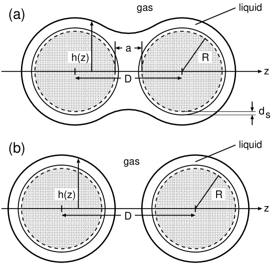
FIG. 1.: Wetting film (thick full line) surrounding two identical homogeneous spheres of radius $R$ which are separated by a distance $D$. The whole system is rotationally symmetric around the $z$ axis which runs through both centers of mass. The position of the liquid-vapor interface which encloses both spheres is described by a function $h(z)$, i.e., in cylindrical coordinates the sharp interface is given by the manifold $\{{\mathbf{r}}(r_{\perp},\phi,z)=(r_{\perp}\cos\phi,r_{\perp}\sin\phi,z)\in{\mathbb{R}}^{3}|r_{\perp}=h(z)\}$. The origin of the coordinate system is in the middle between the two spheres so that their centers are located at $z=\pm D/2$. $a=D-2R$ is the shortest separation between the surfaces of the spheres. Within the so-called sharp-kink approximation this interface separates a region of constant liquid number density $\rho_{l}$ from the surrounding bulk vapor phase of constant number density $\rho_{g}$. Close to the surfaces of the spheres the repulsive interaction leads to a volume with thickness $d_{s}$ excluded for the centers of the fluid particles. For sufficiently large values of $D$ the bridgelike wetting film configuration shown in (a) breaks up into two disjunct pieces so that $h(z)=0$ for a finite interval around $z=0$ (b).

FIG. 2.: Morphologies of liquidlike wetting layers on two adjacent, identical spheres with radius $R=20\sigma$. The center-of-mass distance between them is $D=50\sigma$. The pictures show cross-sections through the system defined by the plane $y=0$; the system is rotationally symmetric around the $z$ axis (see Fig. 1). The thick full lines denote the liquid-vapor interface, the thin dashed lines the surfaces of the spheres. (a) and (b): layer configuration with and without liquid bridge, respectively, for the temperature $T^{*}=k_{B}T/\epsilon=1.3>T_{tt}^{*}$ and at liquid-vapor coexistence $\Delta\mu=0$. Because of its higher free energy the configuration without bridge is metastable (c.f., Fig. 4). These configurations are characterized by the interaction potential parameters $u_{3}=6.283\epsilon\sigma^{3}$, $u_{9}=0.838\epsilon\sigma^{9}$, and $d_{s}=\sigma$. The temperature is above the thin-thick transition temperature $T_{tt}^{*}\approx 1.271$ for each single sphere. In (c) the interaction parameters and $D$ are the same, but the temperature $T^{*}=1.2$ is below the thin-thick transition temperature $T_{tt}^{*}$, so that the wetting layer around a single sphere is thinner than in (a) and (b). Also at this temperature the bridge configuration is the stable one (c.f., Fig. 4).

FIG. 3.: Morphologies of liquidlike wetting layers on two adjacent, identical spheres with radius $R=50\sigma$, $D=120\sigma$, and for the same choice of interaction parameters as in Fig. 2. The thick full lines denote the liquid-vapor interface, the thin dashed lines the surfaces of the spheres. These pictures magnify the region between the spheres. The temperature is $T^{*}=1.2$, which is above the thin-thick transition temperature $T_{tt}^{*}\approx 1.191$ at coexistence for a single sphere, and the pictures differ with respect to the undersaturation: $\Delta\mu^{*}=\Delta\mu/\epsilon=0.05$ in (a), $0.015$ in (b), and $0.01$ in (c). Between (a) and (b), at $\Delta\mu_{bt}^{*}\approx 0.0235$ the system undergoes the first-order transition from the state without bridge to the state with bridge, and at $\Delta\mu_{tt}^{*}\approx 0.0103$ between (b) and (c) there is a thin-thick transition of the wetting layer around the single spheres which is the remnant of the prewetting transition on the corresponding flat substrate (see, c.f., Fig. 4). Note that in (b) there are six turning points ($\bullet$) of the profile $h(z)$ whereas in (c) there are only two.

FIG. 4.: Temperature-undersaturation phase diagram of wetting layer configurations for two spheres with $R=20\sigma$ at a fixed distance $D=50\sigma$ ($a=10\sigma$). The interaction potential parameters are the same as in Fig. 2. The three configurations shown in Fig. 2(a)-(c) are located at the respective thermodynamic states “a” to “c” ($\blacklozenge$). The line of liquid-vapor coexistence $\Delta\mu=0$ separates the region where in the bulk the vapor phase is stable and the liquid phase is metastable ($-\Delta\mu<0$) from the region where the liquid phase is stable and the vapor phase is metastable ($-\Delta\mu>0$). The dotted “metastability line” (“ml”) separates the region where the liquid phase in the bulk is still metastable $(-\Delta\mu>-\Delta\mu_{ml}(T))$ from the region where only the vapor phase is stable in the bulk $(-\Delta\mu<-\Delta\mu_{ml}(T))$. The liquidlike layer on each individual sphere exhibits a first-order thin-thick transition at $-\Delta\mu=-\Delta\mu_{tt}(T)$ (dashed line “tt”). This line intersects the liquid-vapor coexistence line at $T_{tt}^{*}\approx 1.271$ and ends at a critical point ($\bullet$) in the vapor phase region; $T_{tt,c}^{*}\approx 1.275$ and $-\Delta\mu_{tt,c}^{*}\approx-0.0144$. For the present choice of interaction potential parameters, at lower temperatures and larger undersaturations $-\Delta\mu=-\Delta\mu_{bt}(T)$ (full line “bt”) the first-order bridging transitions between the configurations with bridge $(-\Delta\mu>-\Delta\mu_{bt}(T))$ and without bridge $(-\Delta\mu<-\Delta\mu_{bt}(T))$ occur. This line intersects the coexistence line linearly. Within the sharp-kink approximation the line of bridging transitions happens to be cut off by the “metastability line”; within a more sophisticated approach the line “bt” is expected to end at a critical point, too. The locations of the thin-thick transitions in the phase diagram are practically not affected by the presence of the bridge. The dashed-double-dotted lines ($-\cdot\cdot-$) are metastable extensions of the thin-thick and bridging transition lines, respectively. The dashed-dotted line “p” ($-\cdot-$) is the prewetting line for the corresponding planar substrate. It joins the liquid-vapor coexistence line $\Delta\mu=0$ tangentially at the first-order wetting transition temperature $T_{w}^{*}\approx 1.053$ ($\blacktriangle$) and ends at a critical point ($\blacksquare$) in the vapor phase region. For a discussion of the effects of fluctuations on this mean-field phase diagram see the main text.

FIG. 5.: (a) Dependence of the grand canonical potential $\Omega_{S}$ on the separation $a=D-2R$ and the undersaturation $\Delta\mu$ for the same system as in Figs. 2(c) and 4, i.e., for $R=20\sigma$ and $T^{*}=1.2<T_{tt}^{*}$. The dots indicate the end points of metastable branches. For $a<2d_{s}$ (with $d_{s}=\sigma=0.05R$ here) the excluded volumes around the spheres overlap. In the limit $D\to\infty$ the stable solution is the one without a liquid bridge; in this limit $\Omega_{S}(D\to\infty)=2\Omega_{S}^{(1)}$ is twice the free energy of a single sphere surrounded by a wetting layer. At the separation $D_{bt}$ or $a_{bt}$, where the two free energy branches intersect for a given $\Delta\mu$, a first-order morphological phase transition between a configuration with a liquid bridge and a state without bridge takes place. The equilibrium thickness of the homogeneous wetting layer around a single sphere is $l_{0}\approx 1.3\sigma$, so that $D_{bt}/(R+l_{0})\approx 2.39$; the slight deviation from the prediction of Eqs. (27) and (28) is due to the still rather small size of the spheres. We note that, in contrast to the case shown here, for $T>T_{tt}$ the free energy curve corresponding to the solutions without bridge approaches its asymptote from below. (b) Same as in (a), showing the excess free energy $\Omega_{E}=\Omega_{S}-2\Omega_{S}^{(1)}$. In this presentation the results for the solutions without bridge and for different undersaturations $\Delta\mu$ collapse onto a single line. $\Omega_{E}(D\to\infty)$ decays as $D^{-6}$.

FIG. 6.: Excess free energy $\Omega_{E}=\Omega_{S}-2\Omega_{S}^{(1)}$ for $\Delta\mu=0$ in the limit of large spheres, i.e., $R\gg\sigma$, $\sigma\ll a\approx R$. In this limit the excess free energy branch for the unbridged solution vanishes if it is measured in units of $8\pi R^{2}$. Off two-phase coexistence, i.e., for $\Delta\mu\neq 0$ the branch for the bridged solution is determined only by the contributions $\Omega_{lg}$ (Eq. (20)) and $\Omega_{ex}$ (Eq. (16)) to the free energy. At two-phase coexistence $\Delta\mu$ and $\Omega_{ex}$ vanish so that $\Omega_{E}$ is solely determined by $\Omega_{lg}$. Therefore within the local theory with $\Omega_{lg}^{(loc)}$ (Eq. (21)) the bridged solution is a minimal area surface, i.e., its mean curvature is zero. Since $a\gg d_{s}\approx\sigma$ the excluded volume at small $a$ disappears from the figure. Therefore, compared with the full curve in Fig. 5(b) the potential curve here is effectively shifted to smaller values of $a$. Moreover, the actual minimum of the effective interaction potential at small $a\gtrsim\sigma$ (compare Fig. 5), which is due to the influence of the contributions $\Omega_{ei}$ and $\Omega_{sl}$, is not visible on this scale either. The critical separation for the bridging transition ($\blacklozenge$) is given by $a_{bt}/R\approx 0.32$ (Eqs. (27) and (28)). If the thermodynamic state of the system is driven into the off-coexistence region $\Delta\mu>0$ the whole excess free energy branch for the bridged solution is shifted upwards (compare Fig. 5). For any finite value of $\Delta\mu$, in the limit $R\to\infty$ there is no bridging transition anymore (see the main text).

FIG. 7.: Excess free energy $\Omega_{E}=\Omega_{S}-2\Omega_{S}^{(1)}$ (dashed lines) and excess total free energy $\Omega_{E,tot}=\Omega_{S}-2\Omega_{S}^{(1)}+\Phi$ (full lines) for $\Delta\mu=0$. Here $T^{*}=1.2$ and $R=20\sigma$ so that the dashed lines are identical with the full lines in Fig. 5(b). The dots indicate the end points of metastable branches. The parameters $\epsilon_{ss}$ and $\sigma_{ss}$ of the pair potential between the particles forming the spheres are chosen such that the condition $A_{sf}=\sqrt{A\,A_{ss}}$ for the corresponding Hamaker constants is satisfied. Although the wetting-layer induced potential for the solutions without bridge is repulsive, the total interaction potential including the bare dispersion potential is attractive. For small separations $a$ or $D$ the bare dispersion potential dominates. In the limit $D\to\infty$, i.e., for the configurations without bridge, $\Omega_{E}$ and $\Omega_{E,tot}$ decay as $D^{-6}$ as expected for dispersion interactions.

FIG. 8.: Same as in Fig. 5 but with $\Omega_{tot,im}=\Omega_{S}-\Omega_{sg}$ (a) and with $\Omega_{E,im}=\Omega_{tot,im}-2\Omega_{im}^{(1)}$ (b). We choose again $T^{*}=1.2$, $R=20\sigma$, and the interaction parameters as in the previous figures. The dots indicate the end points of metastable branches. The total interaction potential for index-matched spheres and bulk fluid is again repulsive: since the temperature is below the thin-thick transition temperature $T_{tt}$ the adjacent spheres dislike the presence of additional liquid in their vicinity and therefore it is energetically advantageous to separate them as much as possible. $\Omega_{E,im}$ for the solutions without bridge is smaller than $\Omega_{E}$. However, for the bridged solutions, $\Omega_{E,im}$ and $\Omega_{E}$ as well as the corresponding wetting-induced forces are of almost the same size, respectively.

REFERENCES

- [1] See, e.g., J. P. Hansen and I. R. McDonald, Theory of Simple Liquids, 2nd. Ed. (Academic, London, 1986).
- [2] S. Asakura and F. Oosawa, J. Chem. Phys. 22, 1255 (1954).
- [3] Y. Mao, M. E. Cates, and H. N. W. Lekkerkerker, Physica A 222, 10 (1995).
- [4] B. Götzelmann, R. Evans, and S. Dietrich, Phys. Rev. E 57, 6785 (1998); B. Götzelmann, R. Roth, S. Dietrich, M. Dijkstra, and R. Evans, Europhys. Lett. 47, 398 (1999).
- [5] R. Roth, B. Götzelmann, and S. Dietrich, Phys. Rev. Lett. 83, 448 (1999).
- [6] M. Dijkstra, R. van Roij, and R. Evans, Phys. Rev. Lett. 81, 2268 (1998); ibid 82, 117 (1999); Phys. Rev. E 59, 5744 (1999).
- [7] T. W. Burkhardt and E. Eisenriegler, Phys. Rev. Lett. 74, 3189 (1995); E. Eisenriegler and U. Ritschel, Phys. Rev. B 51, 13717 (1995).
- [8] A. Hanke, F. Schlesener, E. Eisenriegler, and S. Dietrich, Phys. Rev. Lett. 81, 1885 (1998).
- [9] H. Löwen, Phys. Rev. Lett. 74, 1028 (1995); Z. Physik B 97, 269 (1995).
- [10] R. Netz, Phys. Rev. Lett. 76, 3646 (1996).
- [11] S. Dietrich, in Phase Transitions and Critical Phenomena, edited by C. Domb and J. L. Lebowitz (Academic, London, 1988), Vol. 12, p. 1.
- [12] T. Bieker and S. Dietrich, Physica A 252, 85 (1998); ibid 259, 466 (1998); and references therein.
- [13] B. M. Law, J.-M. Petit, and D. Beysens, Phys. Rev. E 57, 5782 (1998); J.-M. Petit, B. M. Law, and D. Beysens, J. Colloid Interface Sci. 202, 441 (1998).
- [14] D. Beysens and D. Estève, Phys. Rev. Lett. 54, 2123 (1985); V. Gurfein, D. Beysens, and F. Perrot, Phys. Rev. A 40, 2543 (1989); J. S. van Duijneveldt and D. Beysens, J. Chem. Phys. 94, 5222 (1991); V. Gurfein, F. Perrot, and D. Beysens, J. Colloid Interface Sci. 149, 373 (1992); T. Narayanan, A. Kumar, E. S. R. Gopal, D. Beysens, P. Guenoun, and G. Zalczer, Phys. Rev. E 48, 1989 (1993); D. Beysens, J.-M. Petit, T. Narayanan, A. Kumar, and M. L. Broide, Ber. Bunsenges. Phys. Chem. 98, 382 (1994); A. Kumar and D. Beysens, Physica A 224, 68 (1996).
- [15] P. D. Gallagher and J. V. Maher, Phys. Rev. A 46, 2012 (1992); M. L. Kurnaz and J. V. Maher, Phys. Rev. E 51, 5916 (1995).
- [16] Z. Király, L. Turi, I. Dékány, K. Bean, and B. Vincent, Colloid Polym. Sci. 274, 779 (1996); and references therein.
- [17] Y. Jayalakshmi and E. W. Kaler, Phys. Rev. Lett. 78, 1379 (1997).
- [18] H. Grüll and B. Woermann, Ber. Bunsenges. Phys. Chem. 101, 814 (1997).
- [19] T. Gil, J. H. Ipsen, and C. F. Tejero, Phys. Rev. E 57, 3123 (1998).
- [20] R. Evans, Adv. Phys. 28, 143 (1979).
- [21] S. Dietrich and M. Napiórkowski, Phys. Rev. A 43, 1861 (1991).
- [22] H. T. Dobbs, G. A. Darbellay, and J. M. Yeomans, Europhys. Lett. 18, 439 (1992).
- [23] H. T. Dobbs and J. M. Yeomans, J. Phys: Condens. Matter 4, 10133 (1992).
- [24] J. D. Weeks, D. Chandler, and H. C. Andersen, J. Chem. Phys. 54, 5237 (1971); H. C. Andersen, J. D. Weeks, and D. Chandler, Phys. Rev. A 4, 1597 (1971).
- [25] N. F. Carnahan and K. E. Starling, J. Chem. Phys. 51, 635 (1969).
- [26] C. Bauer and S. Dietrich, Eur. Phys. J. 10, 767 (1999).
- [27] V. Privman and M. E. Fisher, J. Stat. Phys. 33, 385 (1983); J. Appl. Phys. 57, 3327 (1985).
- [28] M. P. Gelfand and R. Lipowsky, Phys. Rev. B 36, 8725 (1987).
- [29] H. C. Hamaker, Physica 4, 1058 (1937).
- [30] J. Israelachvili, Intermolecular and surface forces, 2nd ed. (Academic, London, 1991).
- [31] M. J. Vold, J. Coll. Sci. 16, 1 (1961).
- [32] D. W. J. Osmond, B. Vincent, and F. A. Waite, J. Colloid Interface Sci. 42, 262 (1973); B. Vincent, J. Colloid Interface Sci. 42, 270 (1973).
- [33] M. Kinoshita, Mol. Phys. 94, 485 (1998); and references therein.
- [34] P. N. Pusey and W. van Megen, Nature 320, 340 (1986).
- [35] W. Poon, P. N. Pusey, and H. Lekkerkerker, Physics World 9, p. 27, April 1996.