Incorporation of Density Matrix Wavefunctions in Monte Carlo Simulations: Application to the Frustrated Heisenberg Model

Abstract

We combine the Density Matrix Technique (DMRG) with Green Function Monte Carlo (GFMC) simulations. Both methods aim to determine the groundstate of a quantum system but have different limitations. The DMRG is most successful in 1-dimensional systems and can only be extended to 2-dimensional systems for strips of limited width. GFMC is not restricted to low dimensions but is limited by the efficiency of the sampling. This limitation is crucial when the system exhibits a so–called sign problem, which on the other hand is not a particular obstacle for the DMRG. We show how to combine the virtues of both methods by using a DMRG wavefunction as guiding wave function for the GFMC. This requires a special representation of the DMRG wavefunction to make the simulations possible within reasonable computational time. As a test case we apply the method to the 2–dimensional frustrated Heisenberg antiferromagnet. By supplementing the branching in GFMC with Stochastic Reconfiguration (SR) we get a stable simulation with a small variance also in the region where the fluctuations due to minus sign problem are maximal. The sensitivity of the results to the choice of the guiding wavefunction is extensively investigated.

We analyse the model as a function of the ratio of the next–nearest to nearest neighbor coupling strength which is a measure for the frustration. In agreement with earlier calculations it is found from the DMRG wavefunction that for small ratios the system orders as a Néel type antiferromagnet and for large ratios as a columnar antiferromagnet. The spin stiffness suggests an intermediate regime without magnetic long range order. The energy curve indicates that the columnar phase is separated from the intermediate phase by a first order transition. The combination of DMRG and GFMC allows to substantiate this picture by calculating also the spin correlations in the system. We observe a pattern of the spin correlations in the intermediate regime which is in–between dimerlike and plaquette type ordering, states that have recently been suggested. It is a state with strong dimerization in one direction and weaker dimerization in the perpendicular direction and thus it lacks the the square symmetry of the plaquette state.

PACS numbers: 75.40.Mg, 75.10.Jm, 02.70.Lq

I Introduction

The Density Matrix Technique (DMRG) has proven to be a very efficient method to determine the groundstate properties of low dimensional systems [1]. For a quantum chain it produces extremely accurate values for the energy and the correlation functions. In two dimensional systems the calculational effort increases rapidly with the size of the system. The most favorable geometry is that of a long small strip. In practice the width of the strip is limited to around 8 to 10 lattice sites. Greens Function Monte Carlo (GFMC) is not directly limited by the size of the system but by the efficiency of the importance sampling. When the system has a minus sign problem the statistics is ruined in the long run and accurate estimates are impossible. Many proposals [2] have been made to alleviate or avoid the minus sign problem with varying success, but all of them introduce uncontrollable errors in the sampling. In the DMRG calculation of the wavefunction the minus sign problem is not manifestly present. In all proposed cures of the minus sign problem the errors decrease when the guiding wavefunction approaches the groundstate.

The idea of this paper is that DMRG wavefunctions are much better, also for larger systems, than the educated guesses which usually feature as guiding wave functions. Moreover DMRG is a general technique to construct a wavefunction without knowing too much about the nature of the groundstate, with the possibility to systematically increase the accuracy. Thus DMRG wavefunctions would do very well when they could be used as guiding functions in the importance sampling of the GFMC. There is a complicating factor which prevents a straightforward implementation of this idea due to the fact that interesting systems are so large that it is impossible to use a wavefunction via a look–up table. The value of the wavefunction in a configuration has to be calculated by an in–line algorithm. This has limited the guiding wavefunctions to simple expressions which are fast to evaluate. Consequently such guiding wavefunctions are not an accurate representation of the true groundstate wavefunction, in particular if the physics of the groundstate is not well understood. In this paper we describe a method to read out the DMRG wavefunction in an efficient way by using a special representation of the DMRG wavefunction.

A second problem is that a good guiding wavefunction alleviates the minus sign problem, but cannot remove it as long as it is not exact. We resolve this dilemma by applying the method of Stochastic Reconfiguration which has recently been proposed by Sorella [3]. The viability of our method is tested for the frustrated Heisenberg model.

The behavior of the Heisenberg antiferromagnet has been intruiging for a long time and still is in the center of research. The groundstate of the antiferromagnetic 1-dimensional chain with nearest neighbor coupling is exactly known. In higher dimensions only approximate theories or simulation results are available. The source of the complexity of the groundstate are the large quantum fluctuations which counteract the tendency of classical ordering. The unfrustrated 2–dimensional Heisenberg antiferromagnet orders in a Néel state and by numerical methods the properties of this state can be analyzed accurately [4]. The situation is worse when the interactions are competing as in a 2-dimensional square lattice with antiferromagnetic nearest neighbor $J_{1}$ and next nearest neighbor $J_{2}$ coupling. This spin system with continuous symmetry can order in 2 dimensions at zero temperature, but it is clear that the magnetic order is frustrated by the opposing tendencies of the two types of interaction. The ratio $J_{2}/J_{1}$ is a convenient parameter for the frustration. For small values the system orders antiferromagnetically in a Néel type arrangement, which accomodates the nearest neighbor interaction. For large ratios a magnetic order in alternating columns of aligned spins (columnar phase) will prevail; in this regime the roles of the two couplings are reversed: the nearest neighbor interaction frustrates the order imposed by the next nearest neighbor interaction. In between, for ratios of the order of 0.5, the frustration is maximal and it is not clear which sort of groundstate results. This problem has been attacked by various methods but not yet by DMRG and only very recently by GFMC [5]. This paper addresses the issue by studying the spin correlations.

A simple road to the answer is not possible since the behavior of the system with frustration presents some fundamental problems. The most severe obstacle is that frustration implies a sign problem which prevents the straightforward use of the GFMC simulation technique. Moreover the frustration substantially complicates the structure of the groundstate wavefunction. Generally frustration encourages the formation of local structures such as dimers and plaquettes which are at odds, but not incompatible, with long range magnetic order. These correlation patterns are the most interesting part of the intermediate phase and the main goal of this investigation.

Many attempts have been made to clarify the situation. Often simple approximations such as mean–field or spin–wave theory give useful information about the qualitative behavior of the phase diagram. A fairly sophistocated mean–field theory using the Schwinger boson representation does not give an intermediate phase [6]. Given the complexity of the phase diagram and the subtlety of the effects it is not clear whether such approximate methods can give in this case a reliable clue to the qualitative behavior of the system.

Exact calculations have been performed on small systems up to size $6\times 6$ by Schulz et al. [7]. Although this information is very accurate and unbiased to possible phases, the extrapolation to larger systems is a long way, the more so in view of indications that the anticipated finite size behavior only applies for larger systems. Another drawback of these small systems is that the groundstate is assumed to have the full symmetry of the lattice. Therefore the symmetry breaking, associated with the formation of dimers, ladders or plaquettes, which is typical for the intermediate state, can not be observed directly.

More convincing are the systematic series expansion as reported recently by Kotov et al. [8],[9] and by Singh et al. [10], which bear on an infinite system. They start with an independent dimers (plaquettes) and study the series expansion in the coupling between the dimers (plaquettes). By the choice of the state, around which the perturbation expansion is made, the type of spatial symmetry breaking is fixed. These studies favor in the intermediate regime the dimer state over the plaquette state. Their dimer state has dimers organized in ladders in which the chains and the rungs have nearly equal strength. So the system breaks the translational invariance only in one direction. The energy differences are however small and the series is finite, so further investigation is useful. Our simulations yield correlations in good agreement with theirs, but do not confirm the picture of translational invariant ladders. Instead we find an additional weaker symmetry breaking along the ladders, such that we come closer to the plaquette picture.

Very recently Capriotti and Sorella [5] have carried out a GFMC simulation for $J_{2}=0.5J_{1}$ and have studied the susceptibilities for the orientational and translational symmetry breaking. They conclude that the groundstate is a plaquette state with full symmetry between the horizontal and vertical direction.

From the purely theoretical side the problem has been discussed by Sachdev and Read [11] on the basis of a large spin expansion. From their analysis a scenario emerges in which the Néel phase disappears upon increasing frustration in a continuous way. Then a gapped spatial–inhomogeneous phase with dimerlike correlations appears. For even higher frustration ratios a first order transition takes place to the columnar phase. Although this scenario is qualitative, without precise location of the phase transition points, it definitively excludes dimer formation in the magnetically ordered Néel and columnar phase. It is remarkable that two quite different order parameters (the magnetic order and the dimer order) disappear simultaneously and continuously on opposite sides of the phase transition. In this scenario, this is taken as an indication of some kind of duality of the two phases.

Given all these predictions it is of utmost interest to further study the nature of the intermediate state. Due to the smallness of the differences in energy between the various possibilities, the energy will not be the ideal test for the phase diagram. Therefore we have decided to focus directly on the spin correlations as a function of the ratio $J_{2}/J_{1}$. In this paper we first investigate the 2–dimensional frustrated Heisenberg model by constructing the DMRG wave function of the groundstate for long strips up to a width of 8 sites. The groundstate energy and the spin stiffness which are calculated, confirm the overal picture described above, but the results are not accurate enough to allow for a conclusive extrapolation to larger systems. Then we study an open 10x10 lattice by means of the GFMC technique using DMRG wavefunctions as guiding wavefunction for the importance sampling. The GFMC are supplemented with Stochastic Reconfiguration as proposed by Sorella [3] as an extension of the Fixed Node technique [12]. This method avoids the minus sign problem by replacing the walkers regularly by a new set of positive sign with the same statistical properties. The first observation is that GFMC improves the energy of the DMRG in a substantial and systematic way as can be tested in the unfrustrated model where sufficient information is available from different sources. Secondly the spin correlations become more accurate and less dependent on the technique used for constructing the DMRG wavefunction. The DMRG technique is focussed on the energy of the system and less on the correlations. The GFMC probes mostly the local correlations of the system as all the moves are small and correspond to local changes of the configurations. With these spin correlations we investigate the phase diagram for various values of the frustration ratio $J_{2}/J_{1}$.

The paper begins with the definition of the model to avoid ambiguities. Then a short description of our implementation of the DMRG method is given. We go into more detail about the way how the constructed wavefunctions can be used as guiding wavefunctions in the GFMC simulation. This is a delicate problem since the full construction of a DMRG wavefunction takes several hours on a workstation. Therefore we separate off the construction of the wavefunction and cast it in a form where the configurations can be obtained from each other by matrix operations on a vector. So the length of the computation of the wavefunction in a configuration scales with the square of the number of states included in the DMRG wavefunction. But even then the actual construction of the value of the wavefunction in a given configuration is so time consuming that utmost effiency must be reached in obtaining the wavefunction for successive configurations. The remaining sections are used to outline the GFMC and the Stochastic Reconfiguration and to discuss the results. We concentrate on the correlation functions since we see them as most significant for the structure of the phases. We give first a global evaluation of the correlation function patterns for a wide set of frustration ratios and then focus on a number of points to see the dependence on the guiding wavefunction and to deduce the trends. The paper closes with a discussion and a comparison with other results in the literature.

II The Hamiltonian

The hamiltonian of the system refers to spins on a square lattice.

$${\cal H}=J_{1}\sum_{(i,j)}{\bf S}_{i}\cdot{\bf S}_{j}+J_{2}\sum_{[i,j]}{\bf S}_{i}\cdot{\bf S}_{j}.$$ (1)

The ${\bf S}_{i}$ are spin $\frac{1}{2}$ operators and the sum is over pairs of nearest neigbors $(i,j)$ and over pairs of next nearest neighbors $[i,j]$ on a quadratic lattice. Both coupling constants $J_{1}$ and $J_{2}$ are supposed to be positive. $J_{1}$ tries to align the nearest neigbor spin in an antiferromagnetic way and $J_{2}$ tries to do the same with the next nearest neighbors. So the spin system is frustrated, implying an intrinsic minus sign in the simulations that cannot be gauged away by a rotation of the spin operators.

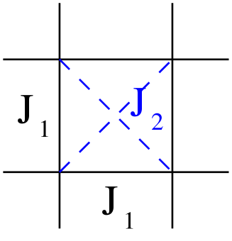
FIG. 1.: The interaction constants $J_{1}$ and $J_{2}$

In order to prepare for the representation of the hamiltonian we express the spin components in spin raising and lowering operators

$${\bf S}_{i}\cdot{\bf S}_{j}=\frac{1}{2}(S^{+}_{i}S^{-}_{j}+S^{-}_{i}S^{+}_{j})+S^{z}_{i}S^{z}_{j}.$$ (2)

We will use the $z$ component representation of the spins and a complete state of the spins will be represented as

$$|R\rangle=|s_{1},s_{2},\cdots,s_{N}\rangle,$$ (3)

where the $s_{j}$ are eigenvalues of the $S^{z}_{j}$ operator. The diagonal matrix elements of the hamiltonian are in the representation (3) given by

$$\langle R|{\cal H}|R\rangle=J_{1}\sum_{(i,j)}s_{i}s_{j}+J_{2}\sum_{[i,j]}s_{i}s_{j}.$$ (4)

The off-diagonal elements are between two nearby configurations $R^{\prime}$ and $R$. $R^{\prime}$ is the same as $R$ except at a pair of nearest neighbors sites $(i,j)$ or next nearest neighbor sites $[i,j]$, for which the spins $s_{i}$ and $s_{j}$ are opposite. In $R^{\prime}$ the pair is turned over by the hamiltonian. Then

$$\langle R^{\prime}|{\cal H}|R\rangle=\frac{1}{2}J_{1}\hskip 28.45274pt{\rm or}\hskip 28.45274pt\langle R^{\prime}|{\cal H}|R\rangle=\frac{1}{2}J_{2},$$ (5)

depending on whether a nearest or a next nearest pair is flipped.

III The DMRG Procedure

The DMRG procedure approximates the groundstate wavefunction by searching through various representations in bases of a given dimension $m$ [1]. Here we take the standard method (with two connecting sites) for granted and make the preparations for the extraction of the wavefunction.

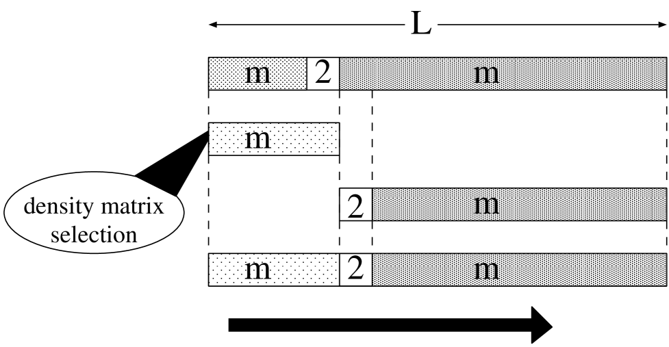
FIG. 2.: The DMRG procedure with one connecting site

The system is mapped onto a 1-dimensional chain (see Fig. 2) and separated into two parts: a left and right hand part. They are connected by one site. Each part is represented in a basis of at most $m$ states. With a representation of all the operators in the hamiltonian in these bases one can find the groundstate of the system. We thus have several representations of the groundstate depending on the way in which the system is divided up into subsystems. The point is to see how these representations are connected and how they possibly can be improved. We take a representation for the right hand parts and improve those on the left. So we assume that for a given division we have the groundstate of the whole system and we want to enlarge the left hand side at the expense of the right hand side. The first step is to include the connecting site in the left hand part. This enlarges the basis for the left hand side from $m$ to $2m$ and a selection has to be made of $m$ basis states. This goes with the help of the density matrix for the left hand side as induced by the wavefunction for the whole system. For later use we write out the basic equations for the density matrix in the configuration representation. Let, at a certain stage in the computation, $|\Phi\rangle$ be the approximation to the groundstate. The configurations of the right hand part and the left hand part are denoted by $R_{r}$ and $R_{l}$. Then the density matrix for the left hand part reads

$$\langle R_{l}|\rho|R^{\prime}_{l}\rangle=\sum_{R_{r}}\langle R_{l},R_{r}|\Phi\rangle\langle\Phi|R^{\prime}_{l},R_{r}\rangle.$$ (6)

In practice we do not solve the eigenvalues of the density matrix in the configuration representation, but in a projection on a smaller basis. White [1] has shown that the best way to represent the state $|\Phi\rangle$ is to select the $m$ eigenstates $|\alpha\rangle$ with the largest eigenvalue

$$\sum_{R^{\prime}_{l}}\langle R_{l}|\rho|R^{\prime}_{l}\rangle\langle R^{\prime}_{l}|\alpha\rangle=\lambda_{\alpha}\langle R_{l}|\alpha\rangle.$$ (7)

The next step is to break up the right hand part into a connecting site and a remainder. With the basis for this remainder and the newly acquired basis for the left hand part we can again compute the groundstate of the whole system as indicated in the lower part of the figure. Now we are in the same position as we started, with the difference that the connecting site has moved one position to the right. Thus we may repeat the cycle till the right hand part is so small that it can exactly be represented by $m$ states or less. Then we have constructed for the left hand part a new set of bases, all containing $m$ states, for system parts of variable length. Next we reverse the roles of left and right and move back in order to improve the bases for the right hand parts with the just constructed bases for the left hand part.

The process may be iterated till it converges towards a steady state. The great virtue of the method is that it is variational. In each step the energy will lower till it saturates. In 1-dimensional system the method has proven to be very accurate [1]. So one wonders what the main trouble is in higher dimensions.

FIG. 3.: Two 1–dimensional paths through the system: “straight” (a) and “meandering” (b).

In Fig. 3 we have drawn 2 possible ways to map the system on a 1-dimensional chain. One sees that if we divide again the chain into a left hand part and a right hand part and a connecting site, quite a few sites of the left hand part are nearest or next nearest neighbors of sites of the right hand part. So the coupling between the two parts of the chain is not only through the connecting site but also through sites which are relatively far away from each other in the 1-dimensional path. The operators for the spins on these sites are not as well represented as those of the connecting site, which is fully represented by the two possible spin states. Yet the correlations between the interacting sites count as much for the energy of the system as those interacting with the connecting site. One may say that the further away two interacting sites are in the 1-dimensional chain the poorer their influence is accounted for. This consideration explains in part why open systems can be calculated more accurately than closed systems, even in 1-dimensional systems.

It is an open question which map of the 2-dimensional onto a 1-dimensional chain gives the best representation of the groundstate of the system. Also other divisions of the system than those suggested by a map on a 1–dimensional chain are possible and we have been experimenting with arrangements which reflect better the 2–dimensional character of the lattice[13]. They are promising but the software for these is not as sophisticated as the one developed by White [14] for the 1-dimensional chain. We therefore have restricted our calculations to the two paths shown here. The second choice. the “meandering” path, was motivated by the fact that it has the strongest correlated sites most nearby in the chain and this choice was indeed justified by a lower energy for a given dimension $m$ of the representation than for the “straight” path.

The DMRG calculations as well as the corresponding GFMC simulations are carried out for both paths. The meandering path has to be preferred over the straight path as the DMRG wavefunctions generally give a better energy value and the simulations suffer less from fluctuations. Nevertheless we have also investigated the straight path, since the path chosen leaves its imprints on the resulting correlation pattern and the paths break the symmetries in different ways. Both paths have an orientational preference. In open systems the translational symmetry is broken anyway, but the meandering path has in addition a staggering in the horizontal direction. This together with the horizontal nearest neighbor sites appearing in the meandering path gives a preference for horizontal dimerlike correlations in this path. On the other hand the straight path prefers the dimers in the vertical direction. Comparing the results of the two choices, allows us to draw further conclusions on the nature of the intermediate state.

IV Extracting configurations from the DMRG wavefunction

It is clear that the wavefunction which results from a DMRG-procedure is quite involved and it is not simple to extract its value for a given configuration. We assume now that the DMRG wavefunction has been obtained by some procedure and we will give below an algorithm to obtain efficiently the value for an arbitrary configuration (see also [13] for an alternative description).

The first step is the construction of a set of representations for the wavefunction in terms of two parts (without a connecting site in between). Let the left hand part contain $l$ sites and the other part $N-l$ sites. We denote the $m$ basis states of the left hand part by the index $\alpha$ and those of the right hand part by $\bar{\alpha}$. The eigenstates of the two parts are closely linked and related as follows

$$\left\{\begin{array}[]{rcl}\langle R_{l}|\alpha\rangle&=&\displaystyle\frac{1}{\sqrt{\lambda_{\alpha}}}\sum_{R_{r}}\langle\Phi|R_{l},R_{r}\rangle\langle R_{r}|\bar{\alpha}\rangle,\\[8.53581pt] \langle R_{r}|\bar{\alpha}\rangle&=&\displaystyle\frac{1}{\sqrt{\lambda_{\alpha}}}\sum_{R_{l}}\langle\alpha|R_{l}\rangle\langle R_{l},R_{r}|\Phi\rangle.\end{array}\right.$$ (8)

It means that for every eigenvalue $\lambda_{\alpha}$ there is and eigenstate $\alpha$ for the left hand part and an $\bar{\alpha}$ for the right hand density matrix. The proof of (8) follows from insertion in the density matrix eigenvalue equation (7).

The second step is a relation for the groundstate wavefunction in terms of these eigenfunctions. Generally we have

$$\langle R_{l},R_{r}|\Phi\rangle=\sum_{\alpha,\bar{\beta}}\langle R_{l}|\alpha\rangle\langle R_{r}|\bar{\beta}\rangle\langle\alpha\bar{\beta}|\Phi\rangle,$$ (9)

while due to (8) we find

$$\begin{array}[]{rcl}\langle\alpha\bar{\beta}|\Phi\rangle&=&\displaystyle\sum_{R_{l},R_{r}}\langle\alpha|R_{l}\rangle\langle\bar{\beta}|R_{r}\rangle\langle R_{l},R_{r}|\Phi\rangle\\[5.69054pt] &=&\displaystyle\sqrt{\lambda_{\alpha}}\sum_{R_{r}}\langle\bar{\beta}|R_{r}\rangle\langle R_{r}|\bar{\alpha}\rangle\ =\delta_{\alpha,\beta}\sqrt{\lambda_{\alpha}}.\end{array}$$ (10)

Thus we can represent the groundstate as

$$\langle R_{l},R_{r}|\Phi\rangle=\sum_{\alpha}\sqrt{\lambda^{l}_{\alpha}}\langle R_{l}|\alpha\rangle_{l}\langle R_{r}|\bar{\alpha}\rangle_{N-l}.$$ (11)

For this part of the problem we have to compute and store the set of $m$ eigenvalues $\lambda^{l}_{\alpha}$ for each division $l$. We point out again that we have on the left hand side the wavefunction and on the right hand side representations for given division $l$, which all lead to the same wavefunction. The last step is to see the connection between these representations.

As intermediary we consider a representation of the wavefunction with one site $s_{l}$ separating the spins $s_{1}\cdots s_{l-1}$ on the left hand side from $s_{l+1}\cdots s_{N}$ on the right hand side. Using the same basis as in (11) we have

$$\begin{array}[]{l}\langle s_{1}\cdots s_{l-1},s_{l},s_{l+1}\cdots s_{N}|\Phi\rangle=\\[5.69054pt] \sum_{\alpha,\alpha^{\prime}}\langle s_{1}\cdots s_{l-1}|\alpha\rangle\phi^{l}_{\alpha,\alpha^{\prime}}(s_{l})\langle s_{l+1}\cdots s_{N}|\bar{\alpha^{\prime}}\rangle.\end{array}$$ (12)

We compare this representation in two ways with (11). First we combine the middle site with the left hand part. This leads to $m$ states which can be expressed as linear combinations of the states of the enlarged segment

$$\sum_{\alpha}\langle s_{1}\cdots s_{l-1}|\alpha\rangle\phi^{l}_{\alpha,\alpha^{\prime}}(s_{l})=\sum_{\alpha^{\prime\prime}}\langle s_{1}\cdots s_{l}|\alpha^{\prime\prime}\rangle T^{l}_{\alpha^{\prime\prime},\alpha^{\prime}}.$$ (13)

In fact this relation is the very essence of the DMRG procedure. The wave function in the larger space is projected on the eigenstates of the the density matrix of that space. Since the process of zipping back forth has converged there is indeed a fixed relation (13). However when we insert (13) into (12) and compare it with (11) we conclude that the matrix $T$ must be diagonal

$$T^{l}_{\alpha^{\prime\prime},\alpha^{\prime}}=\delta_{\alpha^{\prime\prime},\alpha^{\prime}}\sqrt{\lambda^{l}_{\alpha^{\prime}}}.$$ (14)

This leads to the recursion relation

$$\langle s_{1}\cdots s_{l}|\alpha^{\prime}\rangle=\sum_{\alpha}\langle s_{1}\cdots s_{l-1}|\alpha\rangle A^{l}_{\alpha,\alpha^{\prime}}(s_{l})$$ (15)

with

$$A^{l}_{\alpha,\alpha^{\prime}}(s_{l})=\phi^{l}_{\alpha,\alpha^{\prime}}(s_{l})/\sqrt{\lambda^{l}_{\alpha^{\prime}}}.$$ (16)

The second combination concerns the contraction of the middle site with the right hand part. This leads to the recursion relation

$$\langle s_{l}\cdots s_{N}|\bar{\alpha}\rangle=\sum_{\alpha^{\prime}}B^{l-1}_{\alpha,\alpha^{\prime}}(s_{l})\langle s_{l+1}\cdots s_{N}|\bar{\alpha}^{\prime}\rangle$$ (17)

with

$$B^{l-1}_{\alpha,\alpha^{\prime}}(s)=\phi^{l}_{\alpha,\alpha^{\prime}}(s)/\sqrt{\lambda^{l-1}_{\alpha}}.$$ (18)

The $A$ and $B$ matrices are the essential ingredients of the calculation of the wavefunction. From (18) and (16) follows that they are related as

$$B^{l-1}_{\alpha,\alpha^{\prime}}(s)=\sqrt{\lambda^{l}_{\alpha^{\prime}}\,/\,\lambda^{l-1}_{\alpha}}\,A^{l}_{\alpha,\alpha^{\prime}}(s).$$ (19)

By the recursion relations the basis states are expressed as products of $m\times m$ matrices. The determination of the DMRG wavefunction and the matrices $A$ (or $B$) is part of the determination of the DMRG wavefunction which is indeed lengthy but fortunately no part of the simulation. The matrices can be stored and contain the information to calculate the wavefunction for any configuration. The value of the wavefunction is now obtained as the product of matrices acting on a vector. Thus the calculational effort scales with $m^{2}$. Using relation (19) one reconfirms by direct calculation that the wavefunction is indeed independent of the division $l$.

When the simulation is in the configuration $R$, all the $\langle R_{l}|\alpha\rangle_{l}$ and the $\langle R_{r}|\bar{\alpha}\rangle_{N-l}$ are calculated and stored, with the purpose to calculate the wavefunctions more efficiently for the configurations $R^{\prime}$ which are connected to $R$ by the hamiltonian and which are the candidates for a move. The structure of of these nearby states is $R^{\prime}=s_{1}\cdots s_{l_{2}}\cdots s_{l_{1}}\cdots s_{N}\quad(l_{2}>l_{1})$. So we have that for $R^{\prime}$ the representation

$$\langle R^{\prime}|\Phi\rangle=\sum_{\alpha}\sqrt{\lambda^{l_{2}}_{\alpha}}\langle s_{1}\cdots s_{l_{2}}\cdots s_{l_{1}}|\alpha\rangle\langle s_{l_{2}+1}\cdots s_{N}|\bar{\alpha}\rangle$$ (20)

holds. Now we see the advantage of having the wavefunction stored for all the divisions. The second factor in (20) is already tabulated; the first factor involves a number of matrix multiplications equal to the distance in the chain of the two spins $l_{1}$ and $l_{2}$ till one reaches a tabulated function. One can use the tables for a certain number of moves but after a while it starts to pay off to make a fresh list.

V Green Function Monte Carlo simulations

The GFMC technique employs the operator

$${\cal G}=1-\epsilon{\cal H}$$ (21)

and uses the fact that the groundstate $|\Psi_{0}\rangle$ results from

$$|\Psi_{0}\rangle\sim{\cal G}^{n}|\Phi\rangle,\quad\quad\quad\epsilon\ll 1,\quad\quad\quad n\epsilon\gg 1$$ (22)

where in principle $|\Phi\rangle$ may be any function which is non-orthogonal to the groundstate. In view of the possible symmetry breaking, the overlap is a point of serious concern on which we come back in the discussion. In practice we will use the best $|\Phi\rangle$ that we can construct conveniently by the DMRG–procedure described above. The closer $|\Phi\rangle$ is to the groundstate the smaller the number of factors $n$ in the product needs to be in order to find the groundstate. Evaluating (22) in the spin representation gives for the projection on the trial wavefunction the following long product

$$\langle\Phi|\Psi_{0}\rangle\simeq\sum_{\bf R}\langle\Phi|R_{M}\rangle\left[\prod^{M}_{i=1}\langle R_{i}|{\cal G}|R_{i-1}\rangle\right]\langle R_{0}|\Phi\rangle.$$ (23)

Here the sum is over paths ${\bf R}=(R_{M},\cdots R_{1},R_{0})$ which will be generated by a Markov process. The Markov process involves a transition probability $T(R_{i}\leftarrow R_{i-1})$ and the averaging process uses a weight $m(R)$. Its is natural to connect the transition probabilities to the matrix elements of the Greens Function ${\cal G}$. But here comes the sign problem into the game: the transition probabilities have to be positive (and normalized). So we put the transition rate proportional to the absolute value of the matrix element of the Greens Function

$$T(R\leftarrow R^{\prime})=\frac{|\langle R|{\cal G}|R^{\prime}\rangle|}{\sum_{R^{\prime\prime}}|\langle R^{\prime\prime}|{\cal G}|R^{\prime}\rangle|}.$$ (24)

This implies that we have to use a sign function $s(R,R^{\prime})$

$$s(R,R^{\prime})=\frac{\langle R|{\cal G}|R^{\prime}\rangle}{|\langle R|{\cal G}|R^{\prime}\rangle|}$$ (25)

and a weight factor

$$m(R)=\sum_{R^{\prime}}|\langle R^{\prime}|{\cal G}|R\rangle|.$$ (26)

All these factors together form the matrixelement of the Green Function

$$\langle R|{\cal G}|R^{\prime}\rangle=T(R\leftarrow R^{\prime})s(R,R^{\prime})m(R^{\prime}).$$ (27)

If the matrix elements of the Greens Function were all positive, or could be made positive by a suitable transformation, we would not have to introduce the sign function. We leave its consequences to the next section. By the representation (27) we can write the contribution of the path as a product of transition probabilities, signs and local weights. The transition probabilities control the growth of the Markov chain. The signs and weights constitute the weight of a path

$$M({\bf R})=m_{f}(R_{M})\left[\prod^{M}_{i=1}s(R_{i},R_{i-1})m(R_{i-1})\right]m_{i}(R_{0}).$$ (28)

The initial and final weight have to be chosen such that the weight of the paths corresponds to the expansion (23). For the innerproduct $\langle\Phi|\Psi_{0}\rangle$ we get

$$m_{i}(R)=\langle R|\Phi\rangle,\quad\quad\quad m_{f}(R)=\langle\Phi|R\rangle.$$ (29)

With this final weight we have projected the groundstate on the trial wave. This allows us to calculate the so–called mixed averages. For that purpose we define the local estimator ${\cal O}$

$$O(R)=\frac{\langle\Phi|{\cal O}|R\rangle}{\langle\Phi|R\rangle}\,,$$ (30)

which yields the mixed average

$$\langle{\cal O}\rangle_{m}\equiv\frac{\langle\Phi|{\cal O}|\Psi_{0}\rangle}{\langle\Phi|\Psi_{0}\rangle}=\frac{\sum_{{\bf R}}O(R_{M})M({\bf R})}{\sum_{{\bf R}}M({\bf R})}.$$ (31)

For operators not commuting with the hamiltonian the mixed average is an approximation to the groundstate average. Later on we will improve on it.

In this raw form the GFMC would hardly work because all paths are generated with equal weight. One can do better by importance sampling in which one transforms the problem to a Greens Function with matrix elements

$$\langle R|\tilde{{\cal G}}|R^{\prime}\rangle=\frac{\langle\Phi|R\rangle\langle R|{\cal G}|R^{\prime}\rangle}{\langle\Phi|R^{\prime}\rangle}.$$ (32)

Generally this can be seen as a similarity transformation on the operators and from now on everywhere operators with a tilde are related to their counterpart without a tilde as in (32). It gives only a minor change in the formulation. The transition rates are based on the matrix elements of $\tilde{{\cal G}}$ and so are the signs and weights. Thus we have a set of definitions like (24)–(26) with everywhere a tilde on top. It leads also to a change of the initial and final weight

$$\tilde{m}_{i}(R)=|\langle\Phi|R\rangle|^{2},\quad\quad\quad\tilde{m}_{f}(R)=1.$$ (33)

By chosing these weights the formula (30) for the average still applies with a weight $\tilde{M}({\bf R})$ made up as in (28) with the weights and signs with a tilde. Using the tilde operators the local estimator (30) reads

$$O(R)=\sum_{R^{\prime}}\langle R^{\prime}|\tilde{{\cal O}}|R\rangle.$$ (34)

We will speak about the various paths in terms of independent walkers that sample these paths. As some walkers become more important than others in the process, it is wise to improve the variance by branching, which we will discuss later with the sign problem. Before we embark on the discussion of the sign problem we want to summarize a number of aspects of the GFMC simulation relevant to our work.

• The steps in the Markov process are small, only the ones induced by one term of the hamiltonian feature in a transition to a new state. This makes the subsequent states quite correlated. So many steps have to be performed before a statistical independent configuration is reached; on the average a number of the order of the number of sites.

• In every configuration the wave function for a number of neighboring states (the ones which are reachable by the Greens Function), has to be evaluated. This is a time consuming operation and it makes the simulation quite slow, because out of the possibilities (of order $N$) only one is chosen and all the information gathered on the others is virtually useless.

• The necessity to choose a small $\epsilon$ in the Greens Function seems a further slow down of the method, but it can be avoided by the technique of continuous time steps developed by Ceperley and Trivedi [15]. In this method the possibility of staying in the same configuration (the diagonal element of the Greens Function) is eliminated and replaced by a waiting time before a move to another state is made. (For further details in relation to the present paper we refer to [13])

• The average (30) can be improved by replacing it by

  $$\langle{\cal O}\rangle_{im}=2\frac{\langle\Phi|{\cal O}|\Psi_{0}\rangle}{\langle\Phi|\Psi_{0}\rangle}-\frac{\langle\Phi|{\cal O}|\Phi\rangle}{\langle\Phi|\Psi_{0}\rangle}$$ (35)

  of which the error with respect to the true average is of second order in the deviation of $|\Phi\rangle$ from $|\Psi_{0}\rangle$. For conserved operators, such as the energy, this correction is not needed since the the mixed average gives already the correct value.

VI The sign problem and its remedies

In the hamiltonian (1) the $z$ component of the spin operator keeps the spin configuration invariant, whereas the $x$ and $y$ components change the configuration. The typical change is that a pair of nearest or next nearest neighbors is spin reversed. Inspecting the Greens Function it means that all changes to another configuration involve a minus sign! Thus the Greens Function is as far as possible from the ideal of positive matrix elements. The diagonal terms are positive, but they always are positive for sufficiently small $\epsilon$. Importance sampling can remove minus signs in the transition rates, when the ratio of the guiding wavefunction involves also a minus sign. For $J_{2}\neq 0$ no guiding wavefunction can remove the minus sign problem completely. In Fig. 3 we show a loop of two nearest neighbor spin flips followed by a flip in a next nearest neighbor pair, such that the starting configuration is restored. The product of the ratios of the guiding wavefunction drops out in this loop, but the product of the three matrix elements has a minus sign. So at least one of the transitions must involve a minus sign.

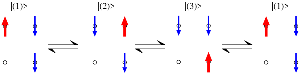
FIG. 4.: Illustration of the sign problem in the frustrated Heisenberg model. The shown sequence of spin flips always involves a sign that can not be gauged away by a different choice of guiding wavefunctions

For unfrustrated systems these loops do not exist and one can remove the minus sign by a transformation of the spin operators

$$S^{x}_{i}\rightarrow-S^{x}_{i},\quad\quad\quad S^{y}_{i}\rightarrow-S^{y}_{i},\quad\quad\quad S^{z}_{i}\rightarrow S^{z}_{i}$$ (36)

which leave the commutation operators invariant. Applying this transformation on every other spin (the white fields of a checkerboard) all flips involving a pair of nearest neighbors then give a positive matrix element for the Greens Function. So when $J_{2}=0$ the appearant sign problem is transformed away. For sufficiently small $J_{2}$, Marshall [16] has shown that the wave function of the system has only positive components (after the “Marshall” sign flip (36)). So the minus sign problem is not due to the wave function but to the frustration. (For the Hubbard model it is the guiding wave function which must have minus signs due to the Pauli principle, while the bare transition probabilities can be taken positive).

Due to the minus sign the weight of a long path picks up a arbitrary sign. Generally the weights are also growing along a path. Thus if various paths are traced out by a number of independent walkers, the average over the paths or the walkers becomes a sum over large terms of both signs, or differently phrased: the average becomes small with respect to the variance; the signal gets lost in the noise.

Ceperley and Alder [12] constructed a method, Fixed Node Monte Carlo (FNMC), which avoids the minus sign problem at the expense of introducing an approximation. Their method is designed for continuum systems and handling fermion wavefunctions. They argued that the configuration space in which the wavefunction has a given sign, say positive, is sufficient for exploring the properties of the groundstate, since the other half of the configuration space contains identical information. Thus they designed a method in which the walkers remain in one domain of a given sign, essentially by forbidding to cross the nodes of the wavefunction. The approximation is that one has to take the nodal structure of the guiding wavefunction for granted and one cannot improve on that, at least not without sophistocation (nodal release). The method is variational in the sense that errors in the nodal structure always raise the groundstate energy.

It seems trivial to take over this idea to the lattice but it is not. The reason is that in continuum systems one can make smaller steps when a walker approaches a node without introducing errors. In a lattice system the configuration space is discrete; so the location of the node is not strictly defined. The important part is that, loosely speaking the nodes are between configurations and one cannot make smaller moves than displacing a particle over a lattice distance or flip a pair of spins. Van Bemmel et al. [17] adapted the FNMC concept to lattice systems preserving its variational character. This extension to the lattice suffers from the same shortcoming as the method of Ceperley and Alder: the “nodal” structure of the guiding wavefunction is given and cannot be improved by the Monte Carlo process. Recently Sorella [3] proposed a modification which overcomes this drawback. It is based on two ingredients.

Sorella noticed that the following effective hamiltonian yields also an upper bound to the energy:

$$\begin{array}[]{rcl}\langle R|\tilde{{\cal H}}_{\rm eff}|R^{\prime}\rangle&=&\left\{\begin{array}[]{rcl}\langle R|\tilde{{\cal H}}|R^{\prime}\rangle&{\rm if}&\langle R|\tilde{{\cal H}}|R^{\prime}\rangle<0\\[5.69054pt] -\gamma\langle R|\tilde{{\cal H}}|R^{\prime}\rangle&{\rm if}&\langle R|\tilde{{\cal H}}|R^{\prime}\rangle>0\quad(\gamma\geq 0)\end{array}\right.\\[17.07164pt] \langle R|\tilde{{\cal H}}_{\rm eff}|R\rangle&=&\langle R|\tilde{{\cal H}}|R\rangle+(1+\gamma)V_{\rm sf}(R)\end{array}$$ (37)

Here the “sign flip” potential is the same as that of ten Haaf et al. [18] and given by

$$V_{\rm sf}(R)=\sum_{R^{\prime}_{\rm na}}\langle R^{\prime}_{\rm na}|\tilde{{\cal H}}|R\rangle$$ (38)

where the subscript “na” (not–allowed) on $R^{\prime}$ restricts the summation to the moves for which the matrix element of the hamiltonian is positive (37).

If the guiding wavefunction were to coincide with the true wavefunction, the simulation of the effective hamiltonian, which is sign free by construction, yields exact averages. So one may expect that good guiding wavefunctions lead to good upperbounds for the energy. This upperbound increases with $\gamma$, indicating that $\gamma=0$ seems the best choice, which is the effective hamiltonian of ten Haaf et al.[18]. That hamiltonian however is a truncated version of the true hamiltonian in which all the dangerous moves are eliminated. The sign flip potential must correct this truncation by suppressing the probability that the walker will stay in a configuration with a large potential.

The second ingredient uses the fact that the hamiltonian (37) explores a larger phase space and therefore contains more information than the truncated one. Parallel to the simulation of the effective hamiltonian one can calculate the weights for the true hamiltonian. As we saw in the summary of the GFMC method, forcefully made positive transition rates still contain the correct weights when supplemented with sign functions. For the true weights of the transition probabilities as given in (37), the “sign function” must be chosen as

$$s(R,R^{\prime})=\left\{\begin{array}[]{lcl}1&{\rm if}&\langle R|\tilde{{\cal H}}|R^{\prime}\rangle>0\\[11.38109pt] -1/\gamma&{\rm if}&\langle R|\tilde{{\cal H}}|R^{\prime}\rangle<0\\[11.38109pt] \displaystyle\frac{1-\epsilon\langle R|\tilde{{\cal H}}|R\rangle}{1-\epsilon\langle R|\tilde{{\cal H}}_{\rm eff}|R\rangle}&{\rm if}&R=R^{\prime}\end{array}\right.$$ (39)

With these “signs” in the weights a proper average can be calculated, but these averages suffer from the sign problem, the more so the smaller $\gamma$ is as one sees from (39). So some intermediate value of $\gamma$ has to be chosen. Fortunately the results are not too sensitively dependent on $\gamma$; the value $\gamma=0.5$ is a good compromise and has been taken in our simulations.

In any simulation some walkers obtain a large weight and others a small one. To lower the variance branching is regularly applied, which means a multiplication of the heavily weighted walkers in favor of the removal of those with small weight. It is not difficult to do this in an unbiased way. Sorella [3] proposed to use the branching much more effectively in conjunction with the signs defined in (39). The average sign is an indicator of the usefulness of the set of walkers. Start with a set of walkers with positive sign. When the average sign becomes unacceptably low, the process is stopped and a reconfiguration takes place. The walkers are replaced by another set with positive weights only, such that a number of measurable quantities gives the same average. The more observables are included the more faithful is the replacement. The construction of the equivalent set requires the solution of a set of linear equations. With the new set of walkers one continues the simulation on the basis of the effective hamiltonian and one keeps track of the true weights with signs. The reconfiguration on the basis of some observables gives at the same time a measure for these obervables. Thus measurement and reconfiguration go together. As the number of observables that can be included is limited some biases are necessarily introduced. Sorella showed that the error in the energy of the guiding wave function is easily reduced by a factor of 10, whereas reduction by the FNMC of ten Haaf et al. [18] rather gives only a factor 2.

FIG. 5.: The energy as function of the frustration ratio

VII Results for the DMRG

In this section we give a brief summary of the results of a pure DMRG–calculation. Extensive details can be found in [13]. The systems are strips of widths up to $W=8$ and of various lengths $L$. They are periodic in the small direction and open in the long direction. The periodicity enables us to study the spin stiffness. We have chosen open boundaries in the long direction to avoid the errors in the DMRG wavefunction due to periodic boundaries. Since we have good control of the scaling behavior in $L$ we extrapolate to $L\rightarrow\infty$ [13]. In the small direction we are restricted to $W=2,4,6$ and 8 as odd values are not compatible with the antiferromagnetic character of the system. For wider system sizes the number of states which has to be taken into account exceeds the possiblities of the present workstations. Our criterion is that the value of the energy does not drift anymore appreciably upon the inclusion of more states. This does not mean that the wavefunction is virtually exact, since the energy is a rather insensitive probe for the wavefunction. For instance correlation functions still improve from the inclusion of more states. In Fig. 5 we present the energy as function of the ratio $J_{2}/J_{1}$, for strip widths 4,6 and 8 together with the best extrapolation to infinite width systems. The figure strongly suggests that the infinite system undergoes a first order phase transition around a value 0.6. This can be attributed to the transition to a columnar order (lines of opposite magnetisation). It is impossible to deduce more information from such an energy curve as other phase transitions are likely to be continuous with small differences in energy between the phases.

The spin stiffness can be calculated with the DMRG–wavefunction for systems which are periodic in at least one direction [13].

FIG. 6.: The stiffness ${\bf\rho}_{s}$ as function of the frustration ratio. Finite size extrapolations put the region where $\rho_{s}$ vanishes between 0.38 and 0.62 [7]

The result of the computation is plotted in Fig. 5. One observes a substantial decrease of $\rho_{s}$ in the frustrated region indicating the appearance of a magnetically disordered phase. In contrast to the energy the data do not allow a meaningful extrapolation to large widths. The lack of clear finite size scaling behavior in the regime of small values of $W$ prevents to draw firm conclusions on the disappearence of the stiffness in the middle regime.

For the correlation functions following from the DMRG wavefunction we refer to [13].

VIII Results for GFMC with SR

We now come to the crux of this study: the simulations of the system with GFMC, using the DMRG wavefunctions to guide the importance sampling. All the simulations have been carried out for $10\times 10$ lattice with open boundaries. Standardly we have 6000 walkers and we run the simulations for about $10^{4}$ measurements. These measuring points are not fully independent and the variance is determined by chopping up the simulations into 50-100 groups, often carried out in parallel on different computers. We first give an overall assessment of the correlation function pattern and then analyze some values of the ratio $J_{2}/J_{1}$.

In the first series we have used the guiding wavefunction on the basis of the meandering path Fig. 3(b), because it gives a better energy than the straight option (a) . The number of basis states is $m=75$, which is small enough to carry out the simulations with reasonable speed and large enough that trends begin to manifest themselves. Measurements of a number of correlation functions are made in conjunction with Stochastic Reconfiguration as described in section 7. The details of these calculations are given in Table I. Note that the DMRG guiding wavefunction gives a better energy for the meandering path than for the straight path for values of $J_{2}/J_{1}$ up to 0.6. From 0.7 on this difference is virtually absent. This undoubtly has to do with the change to the columnar state which can equally well be realized by both paths. The value of $\epsilon$ has been chosen as a compromise: independent measurements require a large $\epsilon$ but the minus sign problem requires to apply often Stochastic Reconfiguration i.e. a small $\epsilon$. One sees that in the heavily frustrated region the $\epsilon$ must be taken small. In fact the more detailed calculations for $J_{2}=0.3J_{1}$ and $J_{2}=0.5J_{1}$ were carried out with $\epsilon=0.01$.

In Fig. 6 and 7 we have plotted a sequence of visualizations of the correlations. From top to bottom (zig–zag) they give the correlations for the values of $J_{2}/J_{1}$. In order to highlight the differences a distinction is made between correlations which are above average (solid lines) and below average (broken lines). All nearest neighbor spin correlations shown are negative. In all the pictures one sees the influence of the boundaries on the spin correlations. Only 1/4 of the lattice has been pictured, the other segments follow by symmetry. The upper right corner, which corresponds to the center of the lattice, is the most significant for the behavior of the bulk. The overall trend is that spatial variations in the correlation functions occur in growing size with $J_{2}/J_{1}$. On the side of low $J_{1}/J_{2}$ (Néel phase) one sees dimer patterns in the horizontal direction, they turn over to vertical dimers (around $J_{2}=0.7J_{1}$) and rapidly disappear in the columnar phase. This is again support for the fact that the columnar phase is separated from the intermediate state by a first order phase transition.

Open boundary conditions have the disadvantage of boundary effects, which make it more difficult to distinguish between spontaneous and induced breaking of the translational symmetry. On the other hand for open boundaries, dimers, plaquettes or any other interruption of the translational symmetry have a natural reference frame. The correlations are not only influenced by the boundaries of the system, also the guiding DMRG–wavefunction leaves its imprint on the results. This is mainly due to the fact that we have only mixed estimators for the correlation functions, which show a mix of the guiding wavefunction and the true wavefunction. The improved estimator, used in these pictures, corrects for this effect to linear order in the deviation. The ladder like structure in the DMRG path is reflected in a ladder like pattern in the correlations as an inspection of the correlations in the DMRG wavefunctions (not shown here) reveals. But ladders are clearly also present in the GFMC results shown in the pictures.

In order to eliminate the influence of the guiding wavefunction we scrutinize some of values of $J_{2}/J_{1}$ in more detail, by inspecting how the results depend on the size of the basis in the DMRG wavefunction and on the choice of the DMRG path. Since we are mostly interested in the behavior of the infinite lattice, we discuss mainly the behavior of the correlations in and around the central plaquette. So we study a sequence of DMRG wavefunctions for $m=32$, 75, 100, 128 and 150(200) and carry out for each of them extensive GFMC simulations. First we look to the case $J_{2}=0$, which is easy because we know that it must be Néel ordered and therefore it serves as a check on the calculations. Then we take $J_{2}=0.3J_{1}$ which is the most difficult case since it is likely to be close to a phase transition. Finally we inspect $J_{2}=0.5J_{1}$ where we are fairly sure that some dimerlike phase is realized.

A $J_{2}=0$

For the unfrustrated Heisenberg model we have several checkpoints for our calculations. We can find to a high degree of accuracy the groundstate energy and we are sure that the Néel phase is homogeneous, i.e. that the correlations show no spatial variation other than that of the antiferromagnet. We have two ways of estimating the energy of a $10\times 10$ lattice. The first method is based on finite size interpolation. From DMRG calculations [13] we have an exact value for a $4\times 4$ lattice, an accurate value for the $6\times 6$ lattice and a good value for the $8\times 8$ lattice. There is also the very accurate calculation of Sandvik [4] for an infinitely large lattice, yielding the value of $e_{0}=-0.669437(5)$. The leading finite size correction goes as $1/L$. Including also a $1/L^{2}$ term we have esimated the value for a $10\times 10$ lattice as 0.629(1) and incorporated this value in Table II(a). We stress that this is an interpolation for which the value of Sandvik is the most important input.

The second method is less well founded and uses the experience that DMRG energy estimates can be improved considerably by extrapolating to zero truncation error. When plotted as function of this truncation error the energy is often remarkably linear. In Table II(b) we give for a series of bases $m=32,75,100,128$ and 150, the values of the truncation error and the corresponding DMRG energy per site together with the extrapolation on the basis of linear behavior. Note that the two estimates are compatible. In Table II(b) we have also listed the values of the GFMC simulations for the corresponding values of $m$. They do agree quite well with these estimates in particular with the one based on finite size scaling. We point out that one would have to go very far in the number of states in the DMRG calculation to obtain an accuracy that is easily obtained with GFMC. Thus the combination of GFMC and DMRG does really better than the individual components. One might wonder why there is still a drift to lower energy values in the GFMC simulations (which is also present in the tables to come). The reason is that the DMRG wavefunction is strictly zero outside a certain domain of configurations, because the truncation of the basis involves also the elimination of certain combinations of conserved quantities of the constituing parts. The domain of the wavefunction grows with the size of the basis.

Turning now to the correlations it seems that they are homogeneous in the center of the lattice for $J_{2}=0$. However a closer inspection reveals small differences. In Table III we list the asymmetries in the horizontal and vertical directions of the spin correlations in and around the central plaquette as function of the number of states. If we number the spins on the lattice as ${\bf S}_{n,m}$ with $1\leq n,m\leq 10$, the central plaquette has the coordinates (5,5), (5,6), (6,5) and (6,6). We then define the asymmetry parameters $\Delta_{x}$ and $\Delta_{y}$ as

$$\left\{\begin{array}[]{l}\Delta_{x}=\frac{1}{4}\langle{\bf S}_{4,5}\cdot{\bf S}_{5,5}+{\bf S}_{4,6}\cdot{\bf S}_{5,6}+{\bf S}_{6,5}\cdot{\bf S}_{7,5}+{\bf S}_{6,6}\cdot{\bf S}_{7,6}\rangle-\frac{1}{2}\langle{\bf S}_{5,5}\cdot{\bf S}_{6,5}+{\bf S}_{5,6}\cdot{\bf S}_{6,6}\rangle\\[5.69054pt] \Delta_{y}=\frac{1}{4}\langle{\bf S}_{5,4}\cdot{\bf S}_{5,5}+{\bf S}_{6,4}\cdot{\bf S}_{6,5}+{\bf S}_{5,6}\cdot{\bf S}_{5,7}+{\bf S}_{6,6}\cdot{\bf S}_{6,7}\rangle-\frac{1}{2}\langle{\bf S}_{5,5}\cdot{\bf S}_{5,6}+{\bf S}_{6,5}\cdot{\bf S}_{6,6}\rangle\end{array}\right.$$ (40)

So $\Delta_{x}$ is the average value of the correlations on the 4 horizontal bonds which are connected to the central plaquette minus the average of the values on the 2 horizontal bonds in the plaquette. Similarly $\Delta_{y}$ corresponds to the vertical direction. The values for the asymmetry in Table III in the vertical direction are so small that they have no significance. Note that the anticipated decrease in $\Delta_{x}$ is slow in DMRG and therefore also slow in the mixed estimator of the GFMC. The improved estimator (35) however is truely an improvement! So one sees that all the observed small deviations from the homogeneous state will disappear with the increase of the number of states in the basis of the DMRG wavefunction. (In general the accuracy of the correlations is determined by that of the GFMC simulations. We get as variance a number of the order 0.01, implying twice that value for the improved estimator)   The vanishing of $\Delta_{x}$ and $\Delta_{y}$ also prove that finite size effects are small in the center of the $10\times 10$ lattice. From these data we may conclude that the GFMC can make up for the errors in the DMRG wavefunction for a relative low number of basis states. We have not carried out a similar series for the straight path since this will certainly show no dimers as will become clear from the following cases.

B $J_{2}=0.3J_{1}$

This case is the most difficult to analyze since it is expected to be close to a continuous phase transition from the Néel state to a dimerlike state. As is known [19] the DMRG structure of the wavefunction is not very adequate to cope with the long–range correlation in the spins typical for a critical point. In Table IV we have presented the same data as in Table III but now for $J_{2}=0.3$. There is no pattern in the energy as function of the truncation error $\delta$. The decrease of the energy as function of the size of the basis $m$ is in the DMRG wavefunctions is not saturated. The GFMC simulations lead to a notably lower energy and they do hardly show a leveling off as function of the basis of the guiding wavefunction. All these points are indicators that the DMRG wavefunction is rather far from convergence and that more accurate data would require a much larger basis. As far as the staggering in the correlations is concerned the values for $\Delta_{x}$ are significant, also because the simulation results generally increase the values. Those for $\Delta_{y}$ are not small enough to be considered as noise. Given the fact that most authors locate the phase transition at higher values $J_{2}\simeq 0.4J_{1}$ we would expect both $\Delta$’s to vanish. So either the dimerlike state is realized for values as low as $J_{2}=0.3J_{1}$ or dimer formation already starts in the Néel state.

To get more insight in the nature of the groundstate we have also carried out the same set of simulations on the straight path (a) in Fig. 3. This guiding wavefunction shows virtually no formation of dimers in any direction as can be observed from Table V. In spite of the fact that the trends indicated in the table have not come to convergence one may draw a few conclusions from the comparison of the two sets of simulations. The overal impression is that the meandering guiding wavefunction represents a groundstate of a different symmetry as compared to the straight path guiding wavefunction. The meandering wavefunction prefers dimers in the horizontal direction and the straight wavefunction leads to some dimerization in the vertical direction. The difference also shows up in the energy, it is not only large on the DMRG level but it also persists at the GFMC level. We see similar trends in the next case.

C $J_{2}=0.5J_{1}$

By any estimate this value of the next nearest neighbor coupling leads to a dimerlike state if it exists at all. No accurate data are available on the energy of the $10\times 10$ system to compare to our results. In Table VI we list the data for a set of DMRG wavefunctions with bases $m=32$, 75, 100, 128, 150 and 200. The DMRG values of the energy (with exception of the value for $m=32$) can be extrapolated to zero truncation error with the limiting value $E_{0}=-48.4(1)$, which corresponds very well with the level in the GFMC values for larger sizes of the basis. This indicates again that the GFMC simulations can make up for the shortcoming of the DMRG wavefunction. One would indeed have to enlarge the basis to $m$ of the order of 1000 in order to achieve the value of the energy of the simulations which use DMRG guiding wavefunctions with a basis of the order of 100.

The staggering in the correlations expressed by the quantities $\Delta_{x}$ for the horizontal direction and $\Delta_{y}$ for the vertical direction, has values that are significant. If one looks to the contributions of the DMRG wavefunction and the GFMC simulation separately, one observes that the overall values do agree quite well, with the tendency that the GFMC simulations lowers the staggerring in the horizontal direction and slightly increases it in the vertical direction. So we may conclude that indeed in the groundstate of the $J_{2}=0.5J_{1}$ system, the correlations of the spins are not translation invariant but show a staggering. However these results neither confirm the picture that the dimerstate is the lowest (as suggested by Kotov et al. [8]) nor that the plaquettestate is the groundstate (as concluded by Capriotti and Sorella [5]). We comment on these discrepancies further in the discussion.

Again it is worthwhile to compare these results with a simulation on the basis of the straight path (a) in Fig. 3. Here it is manifest that the straight path prefers to have the dimers in the vertical direction. Again the impression is that the straight path leads to a different symmetry as compared to the meandering path. It is not only the different preference in the main direction of the dimers, also the secondary dimerization in the perpendicular direction, notably in the meandering case, is not present in the straight case. The fairly large difference in energy on the DMRG level becomes quite small on the GFMC level.

IX Discussion

We have presented a method to employ the DMRG wavefunctions as guiding wavefunctions for a GFMC simulation of the groundstate. Generally the combination is much better than the two individual methods. The GFMC simulations considerably improve the DMRG wavefunction. In the intermediate regime the properties of the GFMC simulations depend on the guiding wavefunction as the results for two different DMRG guiding wavefunctions show.

The method has been used to observe spin correlations in the frustrated Heisenberg model on a square lattice. In this discussion we focus on the intermediate region where the model is most frustrated and which is the “piece de resistance” of the present research. We see patterns of strongly correlated nearest neighbor spins, to be called dimers. To indicate what me mean by strong and weak we give the values in and around the central square of the $10\times 10$ lattice, for the case $J_{2}=0.5J_{1}$. In Fig. 7(c) we have given the values of the central square extrapolated to an infinite lattice.

FIG. 7.: The correlation pattern for the nearest spins for $J_{2}=0.5J_{1}$; (a) according to Kotov et al. [9]: a dimer pattern in which the strength of the correlation is indicated; (b) according to Capriotti and Sorella [5]: a plaquette state and (c) according to this paper: an intermediate pattern in which the translational invariance is broken in both directions but with unequal strength. The values indicated are those based on the meandering path and the improved estimator.

The values are based on the improved estimator and it is interesting to see the trends. The horizontal strong correlation of -0.42 is the result of the DMRG value -0.44 and the GFMC value -0.43, while the weak bond -0.15 is the result of the DMRG value -0.09 and the GFMC value -0.12. Thus the GFMC weakens the order parameter $D_{x}$ associated with the staggering. For the vertical direction there is hardly a change from DMRG to GFMC. One has to go to the next decimal to see the difference. The strong bond equals -0.368 and is coming from the DMRG value -0.375 and the GFMC value -0.371, while the improved weak bond of -0.271 is the resulting value of -0.275 for DMRG and -0.273 for GFMC.

Before we comment on this result we discuss the influence of the choice of the guiding wave function. We note that for both points $J_{2}=0.3J_{1}$ and $J_{2}=0.5J_{1}$ the two choices for the DMRG wavefunction give different results. First of all the main staggering is for the meandering path (b) of Fig. 3 in the horizontal direction, while the straight path (a) of Fig. 3 prefers the dimers in the vertical direction. There is not much difference in the values of the strong and weak correlations. Secondly the straight path shows no appreciable staggering in the other direction, so one may wonder whether the observed effect for the meandering path is real. In our opinion this difference has to do with the effect that the DMRG wavefunction “locks in” on a certain symmetry. The straight path yields a groundstate which is truely dimerlike in the sense that it is translational invariant in the direction perpendicular to the dimers. The meandering path locks in on a different groundstate which holds the middle between a dimerlike and a plaquettelike state. The GFMC simulations cannot overcome this difference in symmetry, likely because the two lowest states with different symmetry are virtually orthogonal. On the DMRG level there is a large difference in energy between the two states, favoring the meandering path strongly, on the GFMC level this difference has become very small. With this observation in mind we compare our result with other findings.

The results of the series expansions [8], [9] and [10] are shown in Fig. 7(a). Their correlations organize themselves in spinladders. The correlations on the rungs of the ladder are $-0.45\pm 0.5$ which compares well with our strongest horizontal correlation and this holds also for the weak horizontal correlation (–0.12 vs –0.15). The most noticeble difference is the value of our weak correlation in the vertical direction (–0.27 vs –0.36) while the strong correlation (–0.37 vs –0.36) agrees. There is no real conflict between our result and theirs since the symmetry they find is fixed by the state around which the series expansion is made. So our claim is only that our state with different symmetry is the lower one. In fact in the paper of Singh et al. [10], it is noted that the susceptibility to a staggering operator in the perpendicular direction (our $\Delta_{y}$) becomes very large in the dimer state for $J_{2}=0.5J_{1}$ which we take as an indication of the nearby lower state. The analytical calculations in [8] and [9] however do not support the existence of the state we find.

Neither do we find support for the plaquette state found in [5], which we have sketched in Fig. 7(b). The evidence of this investigation is based on the boundedness of the susceptibility for the operator which breaks the orientational symmetry and the divergence of the susceptibility for the order parameter breaking translational invariance (corresponding to $\Delta_{x}$). They have not separately investigated the values of $\Delta_{x}$ and $\Delta_{y}$ since their groundstate has the symmetry of the lattice and one would find automatically the same answer. They conclude that in absence of orientational order parameter and with the presence of the translational order parameter the state must be plaquettelike. We believe that their result is influenced by the guiding wavefunction for which the one-step Lanczos approximation is taken. This wavefunction certainly has the symmetry of the square and again GFMC cannot find a groundstate with a different symmetry.

Finally we comment on the fact that we find the dimerization already for values as low as $J_{2}=0.3J_{1}$ at least for the meandering path. As we have mentioned earlier the results as function of the number of states have not sufficiently converged to make a firm conclusion, the more so since there is a large difference between DMRG and GFMC. Still it could be an indication that the phase transition from the Néel state to the dimer state takes place for lower values than the estimated $J_{2}=0.38J_{1}$ [7].

Thus many questions are left over, amongst others how the order parameters behave as function of the frustation ratio in the intermediate region. We feel that the combination of DMRG and GFMC is a good tool to investigate these issues since they demonstrate ad oculos the correlations in the intermediate state.

Acknowledgement The authors are indebted to Steve White for making his software available. One of us (M. S. L. duC. de J.) gratefully acknowledges the hospitality of Steve for a stay at Irvine of 3 months, where the basis of this work was laid. The authors have also benefitted from illuminating discussions with Subir Sachdev and Jan Zaanen. The authors want to acknowledge the efficient help of Michael Patra with the simulations on the cluster of PC’s of the Instituut-Lorentz.

		Straight		Meander
$J_{2}$	$\epsilon$	$E_{\rm DMRG}$	$E_{\rm GFMC}$	$E_{\rm DMRG}$	$E_{\rm GFMC}$
0.0	0.3	-61.30	-62.33(8)	-61.84	-62.54(4)
0.1	0.06	-57.96		-58.53	-59.25(2)
0.2	0.04	-54.75	-56.08(11)	-55.48	-56.22(4)
0.3	0.02	-51.75	-53.17(4)	-52.50	-53.38(3)
0.4	0.02	-49.00	-50.51(8)	-49.92	-50.60(5)
0.5	0.014	-46.68	-47.76(6)	-47.78	-48.34(4)
0.6	0.015	-45.41		-46.03	-46.40(3)
0.7	0.015	-45.67		-45.60	-46.00(2)
0.8	0.02	-49.16		-49.13	-49.60(9)
0.9	0.02	-53.61		-53.70	-54.52(2)
1.0	0.02	-58.46	-59.71(9)	-58.64	-59.80(8)

TABLE I.: For each degree of frustration the imaginary time interval $\epsilon$, the energy of the guiding state $E_{\rm DMRG}$ and that of the GFMC state $E_{\rm GFMC}$ are listed.

$L$	$e_{0}(L\times L)$
4	-0.5740
6	-0.6031
8	-0.6188
10	-0.629(1)
$\infty$	-0.669437(5)

# states	trunc. error	$e_{0}$ (DMRG)	$e_{0}$ (GFMC)
32	21.2 $\times 10^{-5}$	-0.6084	-0.6192(1)
75	12.0 $\times 10^{-5}$	-0.6184	-0.6254(5)
100	10.5 $\times 10^{-5}$	-0.6201	-0.625(2)
128	8.7 $\times 10^{-5}$	-0.6214	-0.6269(6)
150	9.6 $\times 10^{-5}$	-0.6231	-0.6277(5)
$2^{N}$	0	-0.631(3)

(a)                                                              (b)

TABLE II.: Interpolation (a) and extrapolation (b) estimates of the energy per site of a $10\times 10$ lattice

# states	$\Delta_{x}$			$\Delta_{y}$
m	DMRG	GFMC	Improved	DMRG	GFMC	Improved
32	0.14373	0.09981	0.05589	-0.00060	0.00078	0.00216
75	0.07291	0.05668	0.04045	0.00081	0.00601	0.01121
100	0.06432	0.04255	0.03088	0.00030	0.00173	0.00316
128	0.05619	0.03734	0.01849	0.00091	-0.00040	-0.00173
150	0.05044	0.03612	0.02221	0.00079	0.00261	0.00442

TABLE III.: Values for the asymmetry in the center for $J_{2}=0$. As discussed in the text the error in the improved estimator values is of the order 0.02, which means that for $m=128$ and higher the values are statistically indistinguishable from zero.

# states	DMRG				GFMC
$m$	$\delta*10^{5}$	$E_{{\rm DMRG}}$	$\Delta_{x}$	$\Delta_{y}$	$E_{{\rm GFMC}}$	$\Delta_{x}$	$\Delta_{y}$
32	19.0	-51.609	0.27784	0.00295	-52.81(43)	0.363	-0.009
75	10.6	-52.581	0.15462	0.00616	-53.29(05)	0.207	0.011
100	9.4	-52.707	0.14709	0.00943	-53.32(33)	0.145	0.009
128	10.6	-52.821	0.13042	0.00577	-54.01(04)	0.254	0.063
150	10.4	-52.888	0.12564	0.00737	-54.10(12)	0.236	0.103

TABLE IV.: Energies and asymmetries for the case $J_{2}=0.3J_{1}$ as function of the number of basis states $m$. $\delta$ is the truncation error. The asymmetries $\Delta_{x}$ and $\Delta_{y}$ for the GFMC simulations are calculated with the improved estimator. The guiding wavefunction is obtained from the meandering path (b) in Fig. 3. The statistical error in $\Delta_{x}$ and $\Delta_{y}$ is of the order 0.02

# states	DMRG				GFMC
$m$	$\delta*10^{5}$	$E_{{\rm DMRG}}$	$\Delta_{x}$	$\Delta_{y}$	$E_{{\rm GFMC}}$	$\Delta_{x}$	$\Delta_{y}$
32	30.0	-50.672	0.00032	0.01657	-52.15(11)	0.061	0.047
75	18.9	-51.733	-0.00295	0.00426	-53.21(10)	-0.030	0.036
100	19.9	-52.066	0.00349	0.00492	-53.84(72)	0.061	0.079
128	24.6	-52.302	0.00139	0.00791	-53.50(19)	0.079	0.027
150	25.7	-52.455	0.00222	0.00780	-53.52(10)	0.022	0.065

TABLE V.: Comparison of the energies and the values for the asymmetry in the center for the DMRG wavefunction based on the first (straight) path (a) in Fig. 3 and the associated GFMC simulation; $J_{2}=0.3J_{1}$

# states	DMRG				GFMC
$m$	$\delta*10^{5}$	$E_{{\rm DMRG}}$	$\Delta_{x}$	$\Delta_{y}$	$E_{{\rm GFMC}}$	$\Delta_{x}$	$\Delta_{y}$
32	11.8	-47.116	0.43245	0.14667	-47.55(29)	0.295	0.065
75	17.4	-47.771	0.38954	0.13059	-48.22(04)	0.339	0.070
100	12.4	-47.924	0.39364	0.07877	-48.37(22)	0.310	0.110
128	8.4	-48.014	0.37317	0.08246	-48.32(05)	0.336	0.139
150	8.3	-48.088	0.35819	0.07983	-48.33(12)	0.324	0.112
200	7.6	-48.153	0.34590	0.09973	-48.43(05)	0.272	0.094

TABLE VI.: Energies and asymmetries for $J_{2}=0.5J_{1}$ with guiding wavefunction based on the meandering path (b) in Fig. 3

# states	DMRG				GFMC
$m$	$\delta*10^{5}$	$E_{{\rm DMRG}}$	$\Delta_{x}$	$\Delta_{y}$	$E_{{\rm GFMC}}$	$\Delta_{x}$	$\Delta_{y}$
32	69.4	-45.756	0.00172	0.24701	-47.45(08)	0.074	0.185
75	26.2	-46.718	0.00171	0.34950	-47.81(25)	-0.025	0.302
100	21.2	-46.993	0.00063	0.33131	-48.16(06)	-0.003	0.350
128	24.6	-47.231	-0.00029	0.32994	-48.31(08)	0.013	0.291
150	25.7	-47.379	0.00215	0.32458	-48.33(06)	-0.026	0.257

TABLE VII.: Same as Table VI but now for the “straight” path Fig (a) 3

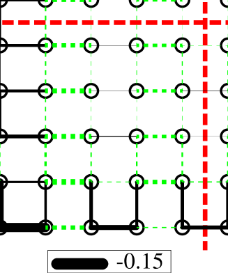
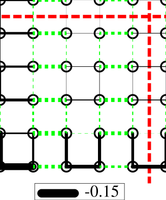
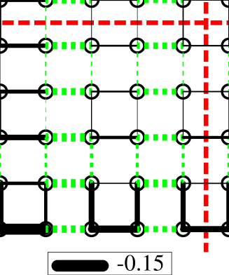
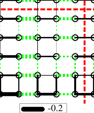
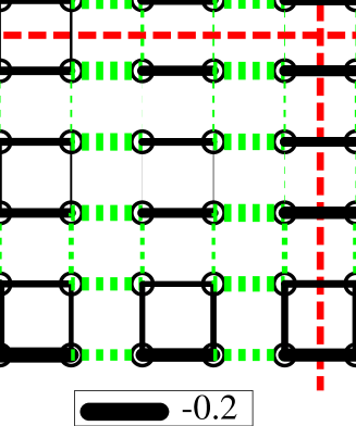
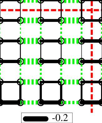
FIG. 8.: The relative correlation strengths on $10\times 10$ lattice. All other nearest neighbour correlations can be obtained by reflection these picture in the two dashed lines. The DMRG guiding state follows the meandering sequence of Fig. 3(b). More explanation is given in the text. Reading zig zag from top left to bottom right, the values for $J_{2}$ are $J_{2}=0,\dots,0.5$ in steps of $0.1$.

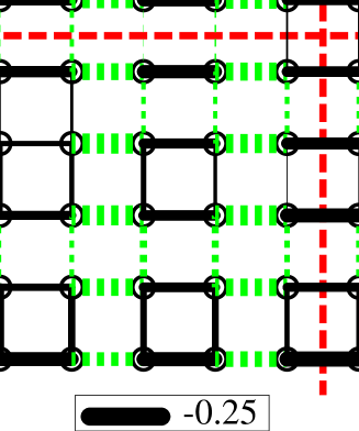
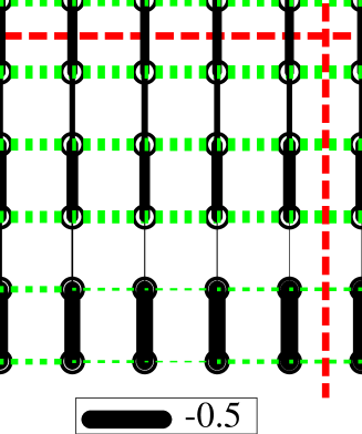
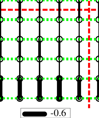
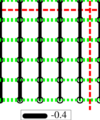
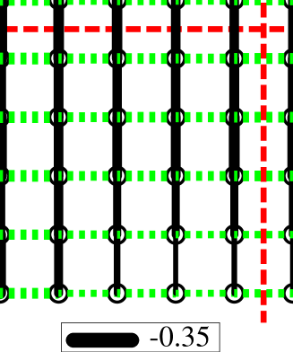
FIG. 9.: The continuation of figure 8; the relative correlation strengths on $10\times 10$ lattice. $J_{2}=0.5,\dots,1.0$ in steps of $0.1$.

REFERENCES

-
[1]
S. R. White, Phys. Rev. Lett. 69 (1992) 2863;
S. R. White, Phys. Rev. B 48(1993) 10345. - [2] For a recent discussion of the sign problem in various cases see P. Henelius and A. W. Sandvik cond–mat/0001351 and references there in.
- [3] S. Sorella, Phys. Rev. Lett. 80 (1998) 4558.
- [4] A. W. Sandvik, Phys. Rev. B56 (1998) 11678.
- [5] L. Capriotti and S. Sorella cond–mat/9911161.
- [6] M. S. L. du Croo de Jongh and P. H. J. Denteneer, Phys. Rev.B 55 (1997) 2713.
- [7] H. J. Schulz, T. A. L. Ziman and D. Poilblanc J. Phys. I 6 (1996) 675.
- [8] V. Kotov, J. Oitmaa, O. P Sushkov and Z. Weihong, Phys. Rev. B 60 (1999) 14613.
- [9] V. Kotov, J. Oitmaa, O. P Sushkov and Z. Weihong, cond–mat/9912228.
- [10] R. R. P. Singh, Z. Weihong, C. J. Hamer and J. Oitmaa, Phys. Rev. B 60 (1999) 7278.
-
[11]
N. Read and S. Sachdev, Phys. Rev. Lett. 62, 1694 (1989).
N. Read and S. Sachdev, Phys. Rev. B 42, 4568 (1990).
N. Read and S. Sachdev, Phys. Rev. Lett. 66, 1773 (1991).
S. Sachdev and N. Read, Int. J. Mod. Phys. B 5, 219 (1991).
S. Sachdev, Quantum Phase Transitions, Cambridge University Press, Cambridge (1999). -
[12]
D. M. Ceperley and B. J. Alder Phys. Rev. Lett.
45(1980) 566;
D. M. Ceperley, Rev. Mod. Phys. 67 (1995) 279. - [13] M. S. L. du Croo de Jongh, Thesis Leiden University 1999, cond-mat/9908200.
- [14] We are grateful to Steve White for making his software available to us.
- [15] N. Trivedi and D. M. Ceperley, Phys. Rev. B 50 (1990) 4552.
- [16] W. Marshall, Proc. Royal Soc. Londen Ser. A 232 (1955) 48.
- [17] H. J. M. van Bemmel, D. F. B. ten Haaf, W. van Saarloos, J. M. J. van Leeuwen and G. An, Phys. Rev. Lett. 72 (1994) 2442.
- [18] D. F. B. ten Haaf, H. J. M. van Bemmel, J. M. J. van Leeuwen, W. van Saarloos and D. M. Ceperley, Phys. Rev. B51 (1995) 13039.
-
[19]
S Östlund and S. Rommer,
Phys. Rev. Lett. 75, 3537 (1995);
S.Rommer and S. Östlund, Phys. Rev. B 55 (1997) 2164.