Partition Function Zeros and Finite Size Scaling
of Helix-Coil Transitions in a Polypeptide

Abstract

We report on multicanonical simulations of the helix-coil transition of a polypeptide. The nature of this transition was studied by calculating partition function zeros and the finite-size scaling of various quantities. New estimates for critical exponents are presented.

A common, ordered structure in proteins is the $\alpha$-helix and it is conjectured that formation of $\alpha$-helices is a key factor in the early stages of protein-folding [1]. It is long known that $\alpha$-helices undergo a sharp transition towards a random coil state when the temperature is increased. The characteristics of this so-called helix-coil transition have been studied extensively [2], most recently in Refs. [3, 4]. They are usually described in the framework of Zimm-Bragg-type theories [5] in which the homopolymers are approximated by a one-dimensional Ising model with the residues as “spins” taking values “helix” or “coil”, and solely local interactions. Hence, in such theories thermodynamic phase transitions are not possible. However, in preliminary work [4] it was shown that our all-atom model of poly-alanine exhibits a phase transition between the ordered helical state and the disordered random-coil state. It was conjectured that this transition is due to long range interactions in our model and the fact that it is not one-dimensional: it is known that the 1D Ising model with long-range interactions also exhibits a phase transition at finite $T$ if the interactions decay like $1/r^{\sigma}$ with $1\leq\sigma<2$ [6]. Our aim now is to investigate this transition in the frame work of a critical theory by means of the finite size scaling (FSS) analysis of partition function zeros. Analysis of partition function zeros is a well-known tool in the study of phase transitions, but was to our knowledge never used before to study biopolymers.

For our project, the use of the multicanonical algorithm [7] was crucial. The various competing interactions within the polymer lead to an energy landscape characterized by a multitude of local minima. Hence, in the low-temperature region, canonical simulations will tend to get trapped in one of these minima and the simulation will not thermalize within the available CPU time. One standard way to overcome this problem is the application of the multicanonical algorithm [7] and other generalized-ensemble techniques [8] to the protein folding problem [9]. For poly-alanine, both the failure of standard Monte Carlo techniques and the superior performance of the multicanonical algorithm are extensively documented in earlier work [10].

In the multicanonical algorithm [7] conformations with energy $E$ are assigned a weight $w_{mu}(E)\propto 1/n(E)$. Here, $n(E)$ is the density of states. A simulation with this weight will lead to a uniform distribution of energy:

$$P_{mu}(E)\,\propto\,n(E)~{}w_{mu}(E)={\rm const}~{}.$$ (1)

This is because the simulation generates a 1D random walk in the energy, allowing itself to escape from any local minimum. Since a large range of energies are sampled, one can use the reweighting techniques [11] to calculate thermodynamic quantities over a wide range of temperatures by

$$<{\cal{A}}>_{T}~{}=~{}\frac{\displaystyle{\int dx~{}{\cal{A}}(x)~{}w^{-1}(E(x))~{}e^{-\beta E(x)}}}{\displaystyle{\int dx~{}w^{-1}(E(x))~{}e^{-\beta E(x)}}}~{},$$ (2)

where $x$ stands for configurations.

It follows from Eq. 1 that the multicanonical algorithm allows us to calculate estimates for the spectral density:

$$n(E)=P_{mu}(E)w^{-1}_{mu}(E)~{}.$$ (3)

We can therefore construct the partition function from these estimates by

$$Z(\beta)=\sum_{E}n(E)u^{E},$$ (4)

where $u=e^{-\beta}$ with $\beta$ the inverse temperature, $\beta=1/k_{B}T$. The complex solutions of the partition function determine the critical behavior of the model. They are the so-called Fisher zeros [12, 13], and correspond to the complex extension of the temperature variable.

Our investigation of the helix-coil transition for poly-alanine is based on a detailed, all-atom representation of that homopolymer, and goes beyond the approximations of the Zimm-Bragg model [5]. The interaction between the atoms was described by a standard force field, ECEPP/2,[14] (as implemented in the KONF90 program [15]) and is given by:

$$E_{tot} = E_{C}+E_{LJ}+E_{HB}+E_{tor},$$ (5)

$$E_{C} = \sum_{(i,j)}\frac{332q_{i}q_{j}}{\epsilon r_{ij}},$$ (6)

$$E_{LJ} = \sum_{(i,j)}\left(\frac{A_{ij}}{r^{12}_{ij}}-\frac{B_{ij}}{r^{6}_{ij}}\right),$$ (7)

$$E_{HB} = \sum_{(i,j)}\left(\frac{C_{ij}}{r^{12}_{ij}}-\frac{D_{ij}}{r^{10}_{ij}}\right),$$ (8)

$$E_{tor} = \sum_{l}U_{l}\left(1\pm\cos(n_{l}\chi_{l})\right).$$ (9)

Here, $r_{ij}$ (in Å) is the distance between the atoms $i$ and $j$, and $\chi_{l}$ is the $l$-th torsion angle. Note that with the electrostatic energy term $E_{C}$ our model contains a long range interaction neglected in the Zimm-Bragg theory [5]. Since one can avoid the complications of electrostatic and hydrogen-bond interactions of side chains with the solvent for alanine (a nonpolar amino acid), explicit solvent molecules were neglected. Chains of up to $N=30$ monomers were considered. We needed between 40,000 sweeps ($N=10$) and 500,000 sweeps ($N=30$) for the weight factor calculations by the iterative procedure described in Refs. [7, 16]. All thermodynamic quantities were estimated from one production run of $N_{sw}$ Monte Carlo sweeps starting from a random initial conformation, i.e. without introducing any bias. We chose $N_{sw}$=400,000, 500,000, 1,000,000, and 3,000,000 sweeps for $N=10$, 15, 20, and 30, respectively.

For our analysis of the partition function zeros we first divide the energy range into intervals of lengths $0.5$ kcal/mol. Equation 4 becomes now a polynomial in the variable $u$ and can be easily solved with MATHEMATICA to obtain all complex zeros $u_{j}^{0}$ ($j=1,2,...$). For the case of $N=10$ we also repeated the calculation of the zeros for energy bin sizes $1.0$ kcal/mol and $0.25$ kcal/mol. The changes in the zeros were smaller than the statistical errors. The effect of the energy bin size on the zeros is also discussed in Ref. [17]. Figure 1 shows the distribution of the zeros for $N=30$ and provides already strong evidence for a singularity on the real axis: in the case of the (analytic) Zimm-Bragg theory the zeros would be located solely on the negative real $u$-axis [18]. We summarize in Table I the leading zeros for each of the four chain lengths, where we have used the mapping $u=e^{-\beta/2}$ due to our binning procedure.

$N$	${\rm Re}\,(u_{1}^{0})$	${\rm Im}\,(u_{1}^{0})$	${\rm Re}\,(\beta_{1}^{0})$	${\rm Im}\,(\beta_{1}^{0})$
10	$0.5620(60)$	$0.0702(33)$	$1.138(21)$	$0.248(11)$
15	$0.6015(23)$	$0.0472(21)$	$1.0104(77)$	$0.1566(67)$
20	$0.6105(29)$	$0.03275(88)$	$0.9842(94)$	$0.1072(26)$
30	$0.6159(19)$	$0.02200(78)$	$0.9681(63)$	$0.0714(25)$

TABLE I.: First partition function zeros for poly-alanine chains of various chain lengths.

The FSS relation by Itzykson et al. [13] for the leading zero $u_{1}^{0}(N)$,

$$u_{1}^{0}(N)=u_{c}+AN^{-1/d\nu}[1+O(N^{y/d})]~{},~{}~{}~{}~{}~{}~{}y<0$$ (10)

shows that the distance from the closest zero $u_{1}^{0}$, to the infinite-chain critical point $u_{c}=e^{-\beta_{c}/2}$ on Re($u$) axis, scales with a relevant linear length $L$, which we translated as $N^{1/d}$ in the above equation. Here, $\beta_{c}$ is the inverse critical temperature of the infinite long polymer chain and $y$ is the correction to scaling exponent. We remark that, unlike in the Zimm-Bragg model, we have no theoretical indication to assume $d$ as a particular integer geometrical dimension and report therefore estimates for the quantity $d\nu$.

For sufficiently large $N$, the exponent $d\nu$ can be obtained from the linear regression

$$-\,{\rm ln}\,|u_{1}^{0}(N)-u_{c}|=\frac{1}{d\nu}\,{\rm ln}(N)+a~{}.$$ (11)

This relation requires an accurate estimate for $u_{c}$. Therefore, we prefer to calculate our estimates for $d\nu$ from the corresponding relation with $|u_{1}^{0}-u_{c}|$ replaced by its imaginary part ${\rm Im}\,u_{1}^{0}$. Including chains of all lengths, $N=10-30$, this approach leads to $d\nu=0.93(5)$, with a goodness of fit $Q=0.48$. Figure 2 displays the corresponding fit. Omitting the smallest chain, i.e. restricting the fit to the range $N=15-30$, does not change the above result. We obtain now $d\nu=0.93(7)$, with $Q=0.22$. This indicates that the $d\nu$ determination is stable over the studied chains and therefore, the correction exponent $y$ can be disregarded in face of the present statistical error.

Considering the real part of the leading zeros given in Table I, ${\rm Re}\,(\beta_{1}^{0}(N))=-{\rm ln}\{[{\rm Re}\,u_{1}^{0}(N)]^{2}\,+[{\rm Im}\,u_{1}^{0}(N)]^{2}\}$, we can derive the critical temperature through the following FSS fit [19],

$${\rm Re}\,(\beta_{1}^{0}(N))=\beta_{c}+bN^{-1/d\nu}~{}.$$ (12)

We obtain $\beta_{c}=0.906(12)$ ($Q=0.005$) for the range $N=10-30$, and $\beta_{c}=0.929(14)$ ($Q=0.63$) for $N=15-30$. The last and more acceptable estimate, corresponds to $T_{c}(\infty)=541(8)$ K.

A stronger version for the relation (10) considers that the next zeros $u_{j}^{0}(N)$, should also satisfy a scaling relation [13],

$$|u_{j}^{0}(N)-u_{c}|\sim\left(\frac{j}{N}\right)^{1/d\nu}~{},$$ (13)

where $j$ labels the zeros in order of increasing distance from $u_{c}$. This relation is expected to be satisfied for large $j$ and allows for an independent check of the estimate for our exponent $d\nu$. The scaling plot in Fig. 3 for the roots closest to the critical point $u_{c}$ demonstrates that the assumed scaling relation is indeed observed for our data as $N$ increases and consistent with our estimate of the exponent $d\nu$.

$N$	$T_{c}$	$C^{max}$	$\Gamma_{C}$	$T_{min}$	$b(T_{min},N)$
10	427(7)	8.9(3)	150(7)	298	-0.48(4)
15	492(5)	12.3(4)	119(5)	429	-0.59(10)
20	508(5)	16.0(8)	88(5)	469	-0.55(8)
30	518(7)	22.8(1.2)	58(4)	500	-0.20(4)

TABLE II.: Numerical results for poly-alanine chains of various lengths: critical temperature $T_{c}$ defined by the maximum of specific heat $C_{max}$, width $\Gamma_{C}$ of peak in specific heat and temperature $T_{min}$ where the Binder cumulant $b(T,N)$ has its minimum, $b(T_{min},N)$.

Our results for the critical temperature and critical exponent can be compared with independent estimates obtained from FSS of the specific heat:

$$C_{N}(T)={\beta}^{2}\ (<E^{2}(T)>-{<E(T)>}^{2})/N~{}.$$ (14)

Defining the critical temperature $T_{c}(N)$ as the position where the specific heat $C_{N}(T)$ has its maximum, we can again calculate the critical temperature by means of Eq. 12. With the values in Table II we obtain $T_{c}(\infty)=544(12)$ K, which is consistent with the value obtained from the partition function zeros analysis, $T_{c}(\infty)=541(8)$ K. Choosing $T_{1}(N)$ and $T_{2}(N)$ such that $C(T_{1})=1/2\,C(T_{c})=C(T_{2})$, we have the following scaling relation for the width $\Gamma_{C}(N)$ of the specific heat [19],

$$\Gamma_{C}(N)=T_{2}(N)-T_{1}(N)\propto N^{-1/d\nu}.$$ (15)

Using the above equation and the values given in Table II, we obtain $d\nu=0.98(11)$ $(Q=0.9)$ for chains of length $N=15$ to $N=30$, i.e. omitting the shortest chain. This value is in agreement with our estimate $d\nu=0.93(5)$, obtained from the partition function zero analysis. Including $N=10$ leads to $d\nu=1.19(10)$, but with a less acceptable fit ($Q=0.1$). The analysis of partition function zeros seems also to be more stable than one relying on Eq. 15. No significant change in $d\nu$ was observed when the data from ref. [4] (which relied on much smaller number of Monte Carlo sweeps) were used in the partition function zeros analysis, while Eq. 15 leads for this reduced statistics to an estimate for $d\nu=1.9$.

Through the scaling relation for the peak of the specific heat, we can evaluate yet another critical exponent, the specific heat exponent $\alpha$, by:

$$C_{N}^{max}\propto N^{\alpha/d\nu}~{}.$$ (16)

In particular, with the values for $C_{N}^{max}$ as given in Table II, we obtain $\alpha=0.86(10)$. The scaling plot for the specific heat is shown in Fig. 4: curves for all lengths of the poly-alanine chains nicely collapse on each other indicating the scaling of the specific heat and the reliability of our exponents. It worths to note that our estimates for $d\nu$ and $\alpha$, as obtained from the finite size scaling of the specific heat, obey within the errorbars the hyperscaling relation $d\nu=2-\alpha$.

It is well-known that renormalization-group fixed point picture leads to a critical exponent $d\nu=1$, $\alpha=1$ and $\gamma=1$ for a first-order phase transition [19, 20, 21]. Our estimate $d\nu=0.93(5)$ for the correlation exponent deviates from unity and rather indicates that the ‘helix-coil-transition” is a strong second order transition. However, the errorbars are such that a first order phase transition cannot be excluded. Our values for the specific heat exponent $\alpha=0.86(10)$ and the susceptibility exponent $\gamma=1.06(14)$ (data not shown) are consistent with a first order phase transition, but also not conclusive. A common way to evaluate the order of a phase transition is by means of the Binder energy cumulant [22],

$$b(T,N)=1-\frac{<E^{4}(T,N)>}{3<E^{2}(T,N)>^{2}}~{}.$$ (17)

For a second order phase transition one would expect that the minimum of this quantity $b(T_{min},\infty)$ approaches $2/3$. Here $T_{min}$ defines the temperature where the cumulant reaches its minimum value and $b(T_{min},\infty)=\lim_{N\rightarrow\infty}b(T,N)$. With the present values of Table II we find the infinite volume extrapolation $b(T_{min},\infty)=0.23(13)$ $(Q=0.12)$, for the range $N=15-30$, which is consistent with a first order phase transition. However, we cannot exclude the possibility of a second order phase transition because the energy cumulant scales with the maximum of specific heat [23], $b(T,N)\sim N^{\alpha/d\nu-1}$, and the true asymptotic limit is reached only for rather large chains due to the value of $\alpha/d\nu$. In fact, the straight line fit for the range $N=10-30$ is less consistent with our data ($Q\simeq 0.001$). Hence, we conclude that our results seem to favor a (weak) first order phase transition, but are not precise enough to exclude the possibility of a second order phase transition.

To summarize, we have used a common technique for investigation of phase transitions, analysis of the finite size scaling of partition function zeros, to evaluate the helix-coil transition in an all-atom model of poly-alanine. Although our results are due to the complexity of the simulated model not precise enough to determine the order of the phase transition, we have demonstrated that the transition can be described by a set of critical exponents. Hence, we have shown for this example that structural transitions in biological molecules can be described within the frame work of a critical theory.

Acknowledgements:
Financial supports from FAPESP and a Research Excellence Fund of the State of Michigan are gratefully acknowledged.

Figure Captions:

1. Partition function zeros in the complex $u$ plane for $N=30$. For the Zimm-Bragg model the zeros would be located solely on the negative real $u$ axis.

2. Linear regression for -ln (Im$\,u^{0}_{1}(N)$) in the range $N=10-30$.

3. Scaling behavior of the first $j$ complex zeros closest to $u_{c}=0.6284$, for chain lengths $N=10,15,20$ and 30.

4. Scaling plot for the specific heat $C_{N}(T)$ as a function of temperature $T$, for poly-alanine molecules of chain lengths $N=10,15,20,$ and $30$.

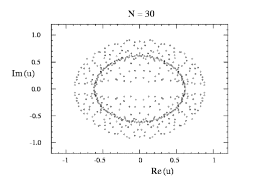
FIG. 1.: Partition function zeros in the complex $u$ plane for $N=30$. For the Zimm-Bragg model the zeros would be located solely on the negative real $u$ axis.

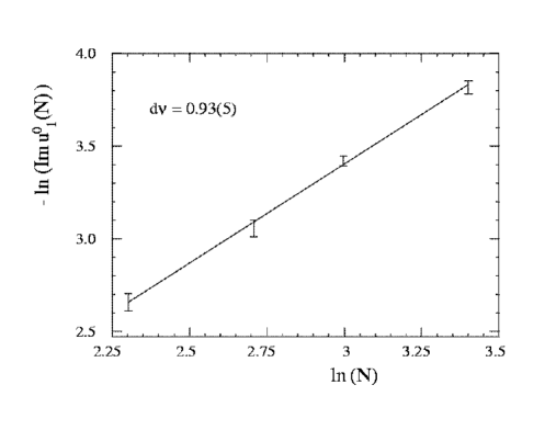
FIG. 2.: Linear regression for -ln (Im$\,u^{0}_{1}(N)$) in the range $N=10-30$.

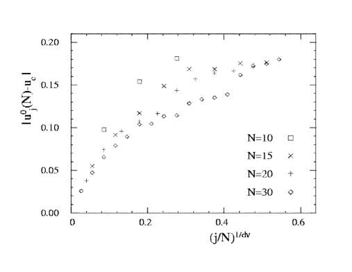
FIG. 3.: Scaling behavior of the first $j$ complex zeros closest to $u_{c}=0.6284$, for chain lengths $N=10,15,20$ and 30.

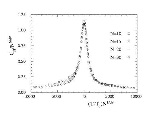
FIG. 4.: Scaling plot for the specific heat $C_{N}(T)$ as a function of temperature $T$, for poly-alanine molecules of chain lengths $N=10,15,20$ and 30.

REFERENCES

- [1] R.M. Ballew, J. Sabelko, and M. Gruebele, Proc. Nat. Acad. Sci. USA 93, 5759 (1996).
- [2] D. Poland and H.A. Scheraga, Theory of Helix-Coil Transitions in Biopolymers (Academic Press, New York, 1970).
- [3] J.P. Kemp and Z.Y. Chen, Phys. Rev. Lett. 81, 3880 (1998).
- [4] U.H.E. Hansmann and Y. Okamoto, J. Chem. Phys. 110, 1267 (1999); 111 1339(E) (1999).
- [5] B.H. Zimm and J.K. Bragg, J. Chem. Phys. 31, 526 (1959).
- [6] F.J. Dyson, Commun. Math. Phys. 12, 212 (1969); J.F. Nagle and J.C. Bonner, J. Phys. C 3, 352 (1970); E. Bayong, H.T. Diep and V. Dotsenko, Phys. Rev. Lett. 83, 14 (1999).
- [7] B.A. Berg and T. Neuhaus, Phys. Lett. B 267, 249 (1991).
- [8] U.H.E. Hansmann and Y. Okamoto, in: Stauffer, D. (ed.) “Annual Reviews in Computational Physics VI” (Singapore: World Scientific), p.129. (1998).
- [9] U.H.E. Hansmann and Y. Okamoto, J. Comp. Chem. 14, 1333 (1993).
- [10] Y. Okamoto and U.H.E. Hansmann, J. Phys. Chem. 99, 11276 (1995).
- [11] A.M. Ferrenberg and R.H. Swendsen, Phys. Rev. Lett. 61, 2635 (1988); Phys. Rev. Lett. 63, 1658(E) (1989), and references given in the erratum.
- [12] M.E. Fisher, in Lectures in Theoretical Physics, vol. 7c p.1 (University of Colorado Press, Boulder, 1965).
- [13] C. Itzykson, R.B. Pearson, and J.B. Zuber, Nucl. Phys. B 220 [FS8], 415 (1983).
- [14] M.J. Sippl, G. Némethy, and H.A. Scheraga, J. Phys. Chem. 88, 6231 (1984), and references therein.
- [15] H. Kawai, Y. Okamoto, M. Fukugita, T. Nakazawa, and T. Kikuchi, Chem. Lett. 1991, 213 (1991); Y. Okamoto, M. Fukugita, T. Nakazawa, and H. Kawai, Protein Engineering 4, 639 (1991).
- [16] U.H.E. Hansmann and Y. Okamoto, Physica A 212, 415 (1994).
- [17] M. Karliner,S.R. Sharpe and Y.F. Chang, Nucl. Phys. B302, 204 (1988).
- [18] V. Matveev and R. Shrock, Phys. Lett. A204, 353 (1995).
- [19] M. Fukugita, H. Mino, M. Okawa and A. Ukawa, J. Stat. Phys. 59, 1397 (1990), and references given therein.
- [20] M.E. Fisher and A.N. Berker, Phys. Rev. B 26, 2507 (1982).
- [21] N.A. Alves, B.A. Berg, and R. Villanova, Phys. Rev. B 43, 5846 (1991).
- [22] K. Binder, Phys. Rev. Lett. 47, 693 (1981).
- [23] N.A. Alves, B.A. Berg, and S. Sanielevici, Phys. Lett. B 241, 557 (1990).