Free Energy Landscape Of Simple Liquids Near The Glass Transition

Abstract

Properties of the free energy landscape in phase space of a dense hard sphere system characterized by a discretized free energy functional of the Ramakrishnan-Yussouff form are investigated numerically. A considerable number of glassy local minima of the free energy are located and the distribution of an appropriately defined “overlap” between minima is calculated. The process of transition from the basin of attraction of a minimum to that of another one is studied using a new “microcanonical” Monte Carlo procedure, leading to a determination of the effective height of free energy barriers that separate different glassy minima. The general appearance of the free energy landscape resembles that of a putting green: deep minima separated by a fairly flat structure. The growth of the effective free-energy barriers with increasing density is consistent with the Vogel-Fulcher law, and this growth is primarily driven by an entropic mechanism.

1 Introduction

A liquid quickly cooled to temperatures below its freezing point enters a metastable supercooled state. At lower temperatures, the supercooled liquid undergoes a glass transition to a state in which it resembles a disordered solid. The dynamics of supercooled liquids near the glass transition exhibits [1, 2] multi-stage, non-exponential decay of fluctuations and a rapid growth of relaxation times, features which are not fully understood.

An intuitive description that is often used [3, 4] for a qualitative understanding of the observed behavior near the glass transition is based on the “free energy landscape” paradigm. This description starts from a functional that expresses the free energy of a liquid in terms of the time-averaged local number density. At high temperatures (or at low densities in systems, such as hard spheres, where the density is the control parameter), this functional is believed to have only one minimum, that representing the uniform liquid state. As the temperature is decreased to near the crystallization point, a new minimum representing the crystal, with a periodic modulation of the local density, should also develop. In the “free energy landscape” picture, a large number of “glassy” local minima of the free energy, characterized by inhomogeneous, aperiodic density distributions, also appear at temperatures below the equilibrium freezing point. If the system gets trapped in one of these glassy local minima as it is cooled rapidly, crystallization can not occur and the subsequent dynamics is governed by thermally activated transitions among some of the many metastable glassy minima. If the system visits many of these minima during its evolution over a certain observation time, it behaves like a liquid over such time scales: the time-averaged local density remains uniform. However, the dynamics in this regime, governed by thermally activated transitions, is slow and complex. In this picture, the glass transition occurs when the time scale of transitions among the glassy minima becomes so long that the system is confined in a single “valley” of the landscape over experimentally accessible time scales. The features of such a free energy landscape would be very similar to those found [5, 6, 7] in certain generalized spin glass models with infinite-range interactions, and in spin models [8, 9] with complicated infinite-range interactions, but no quenched disorder. The behavior of these mean-field models exhibits a remarkable similarity with the phenomenology of the glass transition. These results suggest that the free energy landscape paradigm indeed provides a good framework for the understanding of the properties of supercooled liquids near the glass transition. Such a description requires numerically obtained information about the topography of the free energy landscape of these liquids.

We have carried out several numerical studies of a dense hard-sphere system, using a model free energy functional proposed by Ramakrishnan and Yussouff (RY) [10], a discretized version of which exhibits [11, 12] a large number of glassy local minima at densities higher than the value at which equilibrium crystallization occurs. [The control parameter for a hard-sphere system is the dimensionless density $n^{*}\equiv\rho_{0}\sigma^{3}$, where $\rho_{0}$ is the average number density in the fluid phase and $\sigma$ is the hard-sphere diameter; increasing (decreasing) $n^{*}$ has the same effect as decreasing (increasing) the temperature where the temperature is the control parameter.] From numerical studies [13, 14, 15] of the Langevin equations for this system, we found that the dynamics changes qualitatively at a “crossover” density near $n^{*}_{x}=0.95$. The dynamics of a system initially in the uniform liquid state remains governed by small fluctuations near the liquid free energy minimum when the density is lower than $n^{*}_{x}$. For higher values of $n^{*}$, the dynamics is governed by transitions among the glassy minima. The time scales for such transitions were estimated from a Monte Carlo (MC) method in Ref. [16] and found to increase rapidly with density.

Here we report results of additional numerical studies in which a new approach to the free energy landscape is used. We have developed and used a new MC procedure that enables us to study transitions between different glassy minima and thus investigate the topography of the free energy surface in phase space. We have located a large number of glassy minima of the free energy so as to yield their statistical properties as a function of density. The total number of glassy minima is found to remain nearly constant as the density is varied in the range $0.94\leq n^{*}\leq 1.06$. The free energies of the glassy minima are distributed over a wide range between the free energy of the uniform liquid and that of the crystal. An appropriately defined “overlap” between different glassy minima is also found to exhibit a broad distribution. We have found pairs of glassy minima that differ from each other in the rearrangement of a very small number of particles. The height of the free energy barrier that separates two such minima is quite small. Such pairs may be identified as “two-level systems” which are believed [17] to exist in all glassy systems.

Our computation of the probability of transition from a glassy minimum to the others as a function of the free energy increment (see below) and the MC “time” $t$ leads us to define an effective barrier height that depends weakly on $t$. The growth of this effective barrier height with density is consistent with a Vogel-Fulcher form [18] for a hard-sphere system [19]. The dependence of the effective barrier height on $t$ and the density indicates that the growth of the barrier height (and the consequent growth of the relaxation time) is primarily due to entropic effects arising from an increase in the difficulty of finding low free-energy paths (saddle points) that connect one glassy local minimum with the others.

2 Model and Methods

We characterize our system by a free energy functional $F[\rho]$ of the form [10]:

$$F[\rho] = F_{l}(\rho_{0})+k_{B}T\left[\int{d{\bf r}\{\rho({\bf r})\ln(\rho({\bf r})/\rho_{0})-\delta\rho({\bf r})\}}\right.$$ (1)

$$- \left.(1/2)\int{d{\bf r}\int{d{\bf r}^{\prime}C({|\bf r}-{\bf r^{\prime}|})\delta\rho({\bf r})\delta\rho({\bf r}^{\prime})}}\right],$$

where $F_{l}(\rho_{0})$ is the free energy of the uniform liquid at density $\rho_{0}$, and $\delta\rho({\bf r})\equiv\rho({\bf r})-\rho_{0}$ is the deviation of the density $\rho$ at point ${\bf r}$ from $\rho_{0}$. We set $F_{l}(\rho_{0})=0$. In Eq.(1), $T$ is the temperature and $C(r)$ the direct pair correlation function [20] of the uniform liquid at density $\rho_{0}$, which we express in terms of $n^{*}\equiv\rho_{0}\sigma^{3}$ ($\sigma$ is the hard-sphere diameter) by making use of the Percus-Yevick [20] approximation. The direct pair correlation function [20] of simple model liquids characterized by an isotropic, short-range pair-potential with a strongly repulsive core (such as the Lennard-Jones potential) is very similar to that of the hard-sphere system at high densities. Therefore, we expect our results to apply, at least qualitatively, to such dense liquids.

We discretize our system by introducing a cubic lattice of size $L^{3}$ and mesh constant $h$ in which the variables $\rho_{i},\,i=1,L^{3}$, are defined as $\rho_{i}\equiv\rho({\bf r}_{i})h^{3}$, where $\rho({\bf r}_{i})$ is the density at mesh point $i$. The dimensionless free energy per particle $f[\rho]$ is $f[\rho]=\beta F[\rho]/N$ where $N=\rho_{0}(Lh)^{3}=n^{*}L^{3}a^{3}$ is the total number of particles in the simulation box, $\beta\equiv 1/(k_{B}T)$ and $a$ is the ratio $h/\sigma$.

Ideally, one would like to start the system in a known glassy local minimum of the free energy, and investigate the topography of the free energy surface near the starting point by allowing the system to evolve, and finding out which configurations it subsequently visits and where it ends up. A conventional Metropolis algorithm MC procedure [16] is inefficient at doing this because at the relatively high densities studied here, it would take a very long time for the system to move out of the basin of attraction of the initial minimum. To obviate this difficulty, we have devised what we call a “microcanonical” MC method. The algorithm is as follows: we choose a trial value of what we call the free energy increment, $\Delta F$, or $\Delta f$ if we are dealing with the dimensionless version of $F$. Then, starting with initial conditions which correspond to a local free energy minimum, we sweep the sites $i$ of the lattice sequentially. At each step and site, we pick another site $j$ at random from the ones within a distance $\sigma$ from $i$. We then attempt to change the values of $\rho_{i}$ and $\rho_{j}$ to $p(\rho_{i}+\rho_{j})$ and $(1-p)(\rho_{i}+\rho_{j})$, where $p$ is a random number distributed uniformly in $[0,1]$. The attempted change is accepted, and this is the crucial point, if and only if the free energy after the change is less than $F_{max}\equiv F_{0}+\Delta F$ where $F_{0}$ is the value of the free energy at the minimum where we start the computation. The simulation proceeds up to a maximum “time”, $t_{m}$, measured in MC steps per site (MCS). We perform a sweep over a range of values of $\Delta F$, with the same initial conditions. If $\Delta F$ is smaller than the height of the lowest free energy barrier between the starting minimum and any other “nearby” minima, the system will remain in the basin of attraction of the starting minimum. As we increase $\Delta F$, there will eventually be one or more minima that the system can find within a “time” $t<t_{m}$. These minima are separated from the initial minimum by free energy barriers of height less than $\Delta F$. As $\Delta F$ is further increased, additional minima will be made accessible, and since additional paths will become available between the initial minimum and the minima already accessible at smaller values of $\Delta F$, these minima may be reached in fewer MC steps. Clearly, if one obtains the information of near which minimum the system is, and how long it takes to get there, one can begin to map out the free energy landscape.

To find out which basin of attraction the system is in at time $t$, we save the values of the variables $\rho_{i}$ at relatively frequent time intervals $\Delta t$. These configurations are then used as the inputs in a minimization procedure [11] that determines which basin of attraction the system is in. The entire procedure is repeated a number of times (the “number of runs”) and averaged over. We have carried out this procedure at densities in the range $0.94\leq n^{*}\leq 1.06$. We did not consider densities lower than 0.94 because previous studies [14, 15] show that the dynamics of the system is governed by transitions among glassy local minima only at higher densities. Since the Percus-Yevick approximation becomes less accurate at relatively high densities [20], values of $n^{*}>1.06$ were not considered.

We used two different sets of the sample size $L$ and the mesh size $h$, in one case commensurate with a close-packed lattice, and in the other incommensurate. The computationally more intensive part of our simulations was carried out for systems of size $L=15$ with periodic boundary conditions and mesh size $h=\sigma/4.6$. No crystalline minimum was found for these incommensurate values. The other portion of the computations was performed for systems with $L=12$ and $h=0.25\sigma$. These values are commensurate with a fcc structure and a crystalline minimum is found at sufficiently high densities. Because of the smaller size of these samples, we were able to explore more extensively several aspects of the problem under consideration. Our computations for the $L=15$ sample were carried out for $t_{m}=15000$ MCS and $\Delta t=5000$ MCS, whereas computations for the system with $L=12$ were carried out to $t_{m}=8000$ MCS with $\Delta t=2000$ MCS. A detailed discussion of how the glassy minima used in our study were chosen and the structure of these glassy minima may be found in Refs. [16, 21, 22].

3 Results

During the evolution of the system, we monitor $\beta F$ and the maximum and minimum values of the variables $\rho_{i},i=1,L^{3}$. If the system fluctuates near one of the inhomogeneous minima, then the maximum value of $\rho_{i}$ would be much higher than the value (close to $\rho_{0}h^{3}$) it would have in the vicinity of the uniform liquid minimum. The system does not move to the neighborhood of the liquid minimum for the values of $\Delta F$ considered here. The total free energy remains nearly constant at a value slightly lower than the maximum allowed value, $F_{max}=F_{0}+\Delta F$.

In our analysis of the process of transition of the system from the initial glassy minimum to the basins of other minima, we define a “critical” value, $\Delta f_{c}(t)$ (or $\Delta F_{c}(t)$), of the free-energy increment $\Delta f$ (or $\Delta F$) as follows: at every time investigated (i.e. times 5000, 10000 and 15000 MCS for $L=15$ and times 2000, 4000, 6000 and 8000 MCS for the $L=12$ samples), we test, for increasing values of $\Delta f$, what is the probability, $P(\Delta f,t)$, that the system has moved to the basin of attraction of a free energy minimum distinct from the starting one. This probability, which we obtain by averaging over a sufficient number (ten to fifteen) of runs, is (at constant time) zero for very small $\Delta f$ and rises toward unity as $\Delta f$ increases. At a constant $\Delta f$, it increases somewhat with MC time, as the system explores further regions of phase space. We define $\Delta f_{c}(t)$ as the value of $\Delta f$ for which, at that time, the switching probability reaches $1/2$. Of course, $P$ and $\Delta f_{c}$ are also functions of $n^{*}$. The minima to which the system moves for values of $\Delta f$ close to or higher than $\Delta f_{c}$ are, in general, different for different runs. This suggests that $\Delta f_{c}$ represents a measure of the free energy increment for which a relatively large region of phase space becomes accessible to the system. The system almost never returns to the basin of attraction of the initial minimum: after having left the initial minimum, the system cannot find its way back.

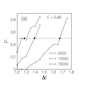
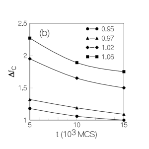
Figure 1: (a) Example of the determination of the “critical” value $\Delta f_{c}$, defined as the value of the free energy increment $\Delta f$ at which the transition probability $P$ is 1/2. The black dots mark the intersections of the plots with the line $P=0.5$ (see text for a complete discussion). The data shown are for a sample of size $L=15$, and three values (5000, 10000 and 15000 MCS) of the Monte Carlo time $t$. (b) Results for $\Delta f_{c}$ as a function of $t$ at four different densities for a $L=15$ minimum. Results for other times and densities studied interpolate smoothly with the results shown.

The procedure for determining $\Delta f_{c}$ is illustrated in Fig. 1a, where we have shown the results for the transition probability $P$ as a function of the free energy increment $\Delta f$ for a $L=15$ minimum at $n^{*}=0.99$. It is clear from our data that the uncertainty in the estimated values of $\Delta f_{c}$ is $\sim 0.05$, the spacing between successive values of $\Delta f$ in the simulation. Typical results for $\Delta f_{c}$ are shown in Fig. 1b for the same $L=15$ minimum and four values of $n^{*}$. Clearly, $\Delta f_{c}$ is a weak function of $t$, and a stronger function of $n^{*}$. The dependence of $\Delta f_{c}$ on $t$ for fixed $n^{*}$ becomes more pronounced as $n^{*}$ is increased. These dependences are analyzed later in this section.

The large number of minimization runs we carried out locate a large fraction of the full collection of glassy minima of the free energy. For the “incommensurate” $L=15$ sample used in our work, the number of minima we have located at each density is in the range of four to six. The “commensurate” $L=12$ sample exhibits a substantially larger number of minima, one of which is crystalline (fcc). A similar sensitivity of the number of local minima to the sample size and boundary conditions has been found in numerical studies [23, 24] of the potential energy landscape of model liquids described by simple Hamiltonians. In the following discussion of the statistical properties of the collection of glassy minima, we consider chiefly the results obtained for $L=12$, for which we can produce significant statistics.

The number of glassy local minima of the $L=12$ system remains nearly constant as the density is varied in the range $0.96\leq n^{*}\leq 1.06$. This number is close to 25. There is no systematic trend in the dependence of this number on the density. The free energies of these minima are distributed in a band that lies between the free energy of the uniform liquid (zero) and that of the crystal. The width of this band increases with $n^{*}$. Since the number of minima is approximately independent of the density, this implies that the “density of states” of the glassy minima decreases as $n^{*}$ is increased. Let $p(\beta F)\delta$ be the probability of finding a glassy minimum with dimensionless free energy between $\beta F-\delta/2$ and $\beta F+\delta/2$. We have calculated this quantity at different values of $n^{*}$. Representative results at two densities, $n^{*}=0.96$ and $n^{*}=1.02$, are shown in Fig. 2a.

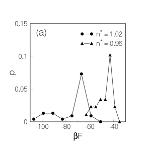
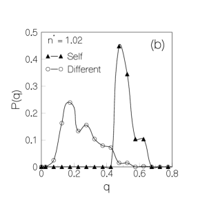
Figure 2: (a) The “density of states” for glassy free energy minima, defined as the probability of finding a glassy minimum with free energy in a given range (see text). Results for $L=12$ samples at two densities are shown. (b) The distribution $P(q)$ of the overlap $q$ defined in Eq.(2). The distributions of the self-overlap and the overlap between different minima are shown separately for $L=12$ samples at density $n^{*}=1.02$.

The values of $\delta$ used are 4.0 and 8.0 for $n^{*}=0.96$ and $n^{*}=1.02$, respectively. The range of $\beta F$ over which $p(\beta F)$ is nonzero is clearly wider at the higher density. The consequent decrease in the values of $p(\beta F)$ with increasing density is also clearly seen. Both distributions show peaks near the upper end, and tails extending to substantially lower values. However, the lowest free energy of the glassy minima is substantially higher than the free energy of the crystalline minimum. If the probability of finding the system in a glassy minimum is assumed to be proportional to the Boltzmann factor $e^{-\beta F}$, then only those minima with free energies lying near the lower end of the band would be relevant in determining the equilibrium and dynamic properties of the system. Our results indicate that the number of such “relevant” minima decreases with increasing $n^{*}$. We find correlations between the free energy of a glassy minimum and its structure, similar to those found in Ref.[14]. Minima with lower free energies have more “structure” (as indicated by e.g. the heights of the first and second peaks of the two-point correlation function of the local density) and higher average density than those with higher free energies.

We have also studied how the distributions of the local density variables in two distinct glassy minima differ from one another. The degree of similarity between two minima may be quantified in terms of their “overlap” [7]. For the discretized system considered here, the overlap $q(1,2)$ between two minima labeled “1” and “2” may be defined in the following way:

$$q(1,2)=\frac{1}{\rho_{av}L^{3}}\,max\{{\bf R}\}\sum_{i}[\rho_{i}^{(1)}-\rho_{av}][\rho_{{\bf R}(i)}^{(2)}-\rho_{av}].$$ (2)

Here, $\rho_{i}^{(1)}$ and $\rho_{i}^{(2)}$ are the discretized densities at the two minima and $\rho_{av}$ is the average value of the $\rho_{i}$, which is assumed to be the same for the two minima. $\bf R$ represents one of the 48 symmetry operations of the cubic mesh, plus all translations taking into account periodic boundary conditions, ${\bf R}(i)$ is the mesh point to which mesh point $i$ is transformed under $\bf R$, and $max\{{\bf R}\}$ means that the $\bf R$ that maximizes the quantity on the right is to be taken. In Fig. 2b, we display the results for the distribution $P(q)$ of $q$ at $n^{*}=1.02$. The distribution of the self-overlap, defined as $q(i,i)$ for the $i$th minimum, is also shown. As expected, the distribution of the self-overlap exhibits a sharp peak at a large value of $q$. The overlap between different minima exhibits a broad distribution with a peak at a small value of $q$, indicating that most of the glassy minima are rather different from one another. This distribution, however, extends to values of $q$ as large as 0.6, indicating that there are a few pairs of glassy minima which are very similar to each other. For each value of $n^{*}$, we find a small number (3-5) of such pairs of minima. The main difference between their structures comes from small displacements of just 2-3 particles. These pairs of minima are examples of “two-level systems” whose existence in glassy materials was postulated [17] many years ago.

We have also looked at how the quantity $F_{c}=F_{0}+\Delta F_{c}$, varies from one minimum to another. While the free energy $F_{0}$ of a glassy minimum varies over a wide range (see Fig. 2a), the value of $F_{c}$ is nearly constant for each value of $n^{*}$. This suggests a “putting green like” free energy landscape in which the local minima are like “holes” of varying depth in a nearly flat background. This structure also implies that there is a strong correlation between the depth of a minimum and the height of the barriers that separate it from the other minima: the barriers are higher for deeper minima.

We now discuss the dependence of $\Delta f_{c}$ on the density $n^{*}$ and MC time $t$. Since the transition probability $P$ is an increasing function of both $\Delta f$ and $t$, $\Delta f_{c}(n^{*},t)$ decreases as $t$ is increased (see Fig. 1). In agreement with the previously observed [16] growth of the barrier-crossing time scale with $n^{*}$, we find that $\Delta f_{c}$ is an increasing function of $n^{*}$. The $t$-dependence of $\Delta f_{c}$ becomes stronger as $n^{*}$ is increased. The $t$-dependence of $\Delta f_{c}$ is closely related to the probability of finding a path (“saddle point”) that connects the starting minimum to a different one. If such paths were relatively easy to find, then the transition probability would be insensitive to the value of $t$ as long as it is not very short. If, however, paths to other minima are few, a large number of configurations have to be explored before one of them is found. The $t$-dependence of $\Delta f_{c}$ would then be more pronounced and extend to larger values of $t$. To make the idea more concrete, we ignore the short-range time correlations among the configurations generated in a MC run and assume that they represent $t$ independent samplings of configurations with free energy less than $F_{0}+\Delta F$. Neglecting the rare return to the basin of attraction of the starting minimum after a transition to a different basin of attraction, the transition probability may then be estimated as $P(n^{*},\Delta f,t)=1-[1-p(n^{*},\Delta f)]^{t}\simeq 1-\exp(-tp)$, where $p(n^{*},\Delta f)\ll 1$ is the probability that a randomly chosen configuration with $\beta F\leq\beta F_{0}+N\Delta f$ belongs in the basin of attraction of a different minimum. One expects $p$ to be zero if $\Delta f\leq\Delta f_{0}(n^{*})$ where $Nk_{B}T\Delta f_{0}$ is the height of the lowest free energy barrier, and $p=g(n^{*},\Delta f-\Delta f_{0})$ for $\Delta f>\Delta f_{0}$ where $g(n^{*},x)$ grows continuously from zero as $x$ is increased from zero. Combining this with the definition of $\Delta f_{c}$, we obtain the relation $g(n^{*},\Delta f_{c}(n^{*},t)-\Delta f_{0}(n^{*}))=\ln 2/t$. Since $\Delta f_{c}(n^{*},t_{1})-\Delta f_{c}(n^{*},t_{2})$ for fixed $t_{1}<t_{2}$ increases with $n^{*}$, the function $g(n^{*},x)$ decreases (i.e. the difficulty of finding paths to other minima increases) as $n^{*}$ is increased at fixed $x$.

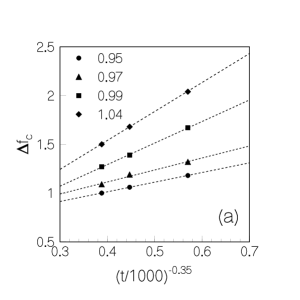
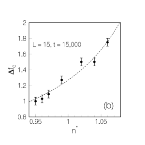
Figure 3: (a) Plots of $\Delta f_{c}$, obtained for a $L$ = 15 minimum, against $(t/1000)^{-0.35}$ for four values of $n^{*}$. The dashed lines are the best straight-line fits. (b) The dependence of $\Delta f_{c}(n^{*},t=15000)$ on $n^{*}$ for $L$ = 15. The dashed line shows the best fit to a Vogel-Fulcher form (see text).

The observed $t$-dependence of $\Delta f_{c}$ for all values of $n^{*}$ and all the minima in our study is well-represented by

$$\Delta f_{c}(n^{*},t)=\Delta f_{0}(n^{*})+c(n^{*})t^{-\alpha},$$ (3)

with $\alpha$ in the range $0.25-0.40$. Fits to this form with $\alpha=0.35$ for a minimum with $L$ = 15 are shown in Fig. 3a. The values of $\Delta f_{0}$ obtained from such fits with a fixed value of $\alpha$ are nearly independent of $n^{*}$, but exhibit a dependence on the value of $\alpha$, varying between 0 and 0.5 for the $L$ = 15 minimum. Similar results are obtained for $L=12$, with values of $\Delta f_{0}$ between 1.3 and 1.5. The quantity $c(n^{*})$ increases with $n^{*}$. These results correspond to $g(n^{*},x)\sim A(n^{*})x^{1/\alpha}$ with $A(n^{*})$ decreasing with increasing $n^{*}$. We conclude that the growth of the effective barrier height with increasing $n^{*}$ is primarily due to an entropic mechanism associated with an increase of the difficulty in finding low-lying saddle points that connect different glassy local minimum of the free energy.

The dependence of $\Delta f_{c}$ on $n^{*}$ is consistent with the Vogel-Fulcher law [18] which assumes the following form [19] for our system:

$$\Delta f_{c}(n^{*})=a+b/(n^{*}_{c}-n^{*}),$$ (4)

where $a$, $b$ and $n^{*}_{c}$ are constants. The value of $n^{*}_{c}$ obtained from fits of our data for $\Delta f_{c}(n^{*},t)$ to Eq.(4) with fixed $a$ is nearly independent of $t$. This is consistent with the form of Eq.(3) if $a=\Delta f_{0}$ , $b\propto t^{-\alpha}$, and $c\propto 1/(n^{*}_{c}-n^{*})$. $\Delta f_{0}$ is indeed nearly independent of $n^{*}$, and we find that the $t$-dependence of $b$ and the $n^{*}$-dependence of $c$ are in agreement with the other two conditions. For the $L$ = 15 case, we can fit the data for $\Delta f_{c}$ at $t$ = 15,000 to the form of Eq.(4) with $a$ = 0 ($\Delta f_{0}=0)$. The best fit, shown in Fig. 3b, corresponds to $n^{*}_{c}=1.225$, very close to the expected random close packing density $n^{*}_{rcp}\simeq 1.23$. The best fit to the $L$ = 12 data with $a\simeq 1.0$ also yields a similar value of $n^{*}_{c}$. We conclude that the observed growth of the effective barrier height is consistent with the Vogel-Fulcher form. The increase in the effective barrier height as $n^{*}$ is increased from 0.96 to 1.06 is about 25$k_{B}T$, corresponding to a growth of the characteristic time scale of about ten orders of magnitude. Thus, the range of time scales covered in our study is comparable to that used in Vogel-Fulcher fits of experimental data, and much wider than what can be achieved in standard MC or molecular dynamics simulations.

4 Discussion

We close with a discussion of the connections between our results and those of spin-glass-like theories [6, 7, 25] of the structural glass transition (see Ref. [22] for a discussion of the relation of our work with other recent studies of the behavior of simple liquids near the glass transition). These theories are based on the similarity between the phenomenology of the structural glass transition in so-called “fragile” [2] liquids and the behavior found in a class of generalized mean-field spin glass models [5, 26] with infinite-range interactions. At high temperatures, the free energy of these mean-field models, expressed as a function of the single-site magnetizations, exhibits only one, “paramagnetic”, minimum. As $T$ is lowered, an exponentially large number of non-trivial local minima come into existence at a temperature $T_{d}$, where a “dynamic transition”, characterized by a breaking of ergodicity, occurs. This “dynamic transition” does not have any signature in the equilibrium behavior of the system. A thermodynamic phase transition occurs at a lower temperature $T_{c}$. In the suggested analogy between these models and the structural glass transition, the paramagnetic minimum of the free energy is identified with that corresponding to the uniform liquid, and the role of the non-trivial local minima of the free energy is played by the glassy local minima. The analogue of the “dynamic transition” at $T_{d}$ is thought to be smeared out in liquids. It has been suggested [6, 7, 25] that $T_{d}$ should be identified with the “ideal glass transition” temperature of mode-coupling theories [27]. The temperature $T_{c}$ is interpreted as the “Kauzmann temperature” [28] at which the difference in entropy between the supercooled liquid and the crystalline solid extrapolates to zero. The relaxation time of the supercooled liquid is supposed to diverge at this temperature. Heuristic arguments suggest that this divergence is of the Vogel-Fulcher form [7, 25].

Our results qualitatively support this scenario. We find a characteristic density at which a large number of glassy minima of the free energy appear. We do not know whether the number of glassy minima depends exponentially on the sample volume. The configurational entropy associated with these minima decreases with increasing density because the width of the band over which the free energy of these minima is distributed increases with density. We have also found evidence for a Vogel-Fulcher-type growth of relaxation times driven by an entropic mechanism.

There are, however, certain differences between our findings and the predictions of spin-glass-like theories. In our earlier work [14, 15], we found that the free energy of a typical glassy minimum becomes lower than that of the uniform liquid as the density is increased slightly above the value ($n^{*}\approx$ 0.8) at which the minimum comes into existence. In particular, the free energies of the glassy minima are substantially lower than that of the uniform liquid one for $n^{*}$ near $n^{*}_{x}\simeq 0.95$, the crossover density [14, 15] above which the dynamics is governed by transitions among glassy minima. This is different from the behavior found in the spin glass models. Our results for the distribution of the overlap between different minima are also somewhat different from those for the spin glass models. Some of these differences may be due to finite-size effects which are probably significant for the small samples considered here. Also, fluctuation effects, which are unimportant in mean-field models, may play an important role in our system. A careful investigation of these issues would be interesting.

References

References

- [1] Jäckle J 1986 Rep. Prog. Phys. 49 171.
- [2] Angell C A 1988 J. Phys. Chem. Solids 49 863.
- [3] Anderson P W 1979 in Ill Condensed Matter, Lecture Notes of the Les Houches Summer School, ed R Balian, R Maynard and G Toulouse (Amsterdam: North Holland).
- [4] Wolynes P G 1988 in Proceedings of International Symposium on Frontiers in Science, (AIP Conf. Proc. No. 180), ed S S Chen and P G Debrunner (New York: American Institute of Physics).
- [5] Kirkpatrick T R and Wolynes P G 1987 Phys. Rev. A 35 3072; Phys. Rev B 36 8552.
- [6] Kirkpatrick T R and Thirumalai D 1989 J. Phys. A 22 L149.
- [7] Kirkpatrick T R, Thirumalai D and Wolynes P G 1989 Phys. Rev. A 40 1045.
- [8] Bouchaud J -P and Mezard M 1994 J. Phys. I (France) 4 1109.
- [9] Cugliandolo L F, Kurchan J, Parisi G and Ritort F 1995 Phys. Rev. Lett. 74 1012.
- [10] Ramakrishnan T V and Yussouff M 1979 Phys. Rev. B 19 2775.
- [11] Dasgupta C 1992 Europhys. Lett. 20 131.
- [12] Dasgupta C and Ramaswamy S 1992 Physica A 186 314.
- [13] Lust L M, Valls O T, and Dasgupta C 1993 Phys. Rev. E 48 1787.
- [14] Dasgupta C and Valls O T 1994 Phys Rev. E 50 3916.
- [15] Valls O T and Dasgupta C 1995 Transport Theory and Stat. Physics 24 1199.
- [16] Dasgupta C and Valls O T 1996 Phys. Rev. E 53 2603.
- [17] Anderson P W, Halperin B I and Varma C M 1972 Philos. Mag. 25 1; Phillips W A 1972 J. Low. Temp. Phys. 7 351.
- [18] Vogel H 1921 Z. Phys. 22 645; Fulcher G S 1925 J. Amer. Ceram. Soc. 8 339.
- [19] Woodcock L V and Angell C A 1981 Phys. Rev. Lett. 47 1129.
- [20] Hansen J P and McDonald I R 1986 Theory of Simple Liquids (London: Academic).
- [21] Dasgupta C and Valls O T 1998 Phys. Rev. E 58 801.
- [22] Dasgupta C and Valls O T 1998 Phys. Rev. E 59 3123.
- [23] Heuer A 1997 Phys. Rev. Lett. 78 4051.
- [24] Daldoss G, Pilla O, Villani G, and Ruocco G, 1998 preprint (cond-mat/9804113).
- [25] Parisi G 1997 in Complex Behaviour of Glassy Systems: Proceedings of the XIV Sitges Conference, ed M Rubi and C Perez-Vicente (Berlin: Springer).
- [26] Kirkpatrick T R and Thirumalai D 1987 Phys. Rev. B 36 5388.
- [27] Götze W 1991 in Liquids, Freezing and the Glass Transition ed J P Hansen, D Levesque and J Zinn-Justin (New York: Elsevier).
- [28] Kauzmann W 1948 Chem. Rev. 48 219.