Multi-scaling properties of truncated Lévy flights

Abstract

Multi-scaling properties of one-dimensional truncated Lévy flights are studied. Due to the broken self-similarity of the distribution of jumps, they are expected to possess multi-scaling properties in contrast to the ordinary Lévy flights. We argue this fact based on a smoothly truncated Lévy distribution, and derive the functional form of the scaling exponents. Specifically, they exhibit bi-fractal behavior, which is the simplest case of multi-scaling.

I Introduction

Lévy flights are random processes based on Lévy stable distributions[1]. They have been utilized successfully in modeling various complex spatio-temporal behavior of non-equilibrium dissipative systems such as fluid turbulence, anomalous diffusion, and financial markets[2].

The Lévy stable distribution is self-similar to its convolutions. It has a long power-law tail that decays much more slowly compared with an exponential decay, which gives rise to infinite variance. However, in practical situations, it is usually truncated due to nonlinearity or finiteness of the system. In order to incorporate this fact, Mantegna and Stanley[3] introduced the notion of truncated Lévy flight. It is based on a truncated Lévy stable distribution with a sharp cut-off in its power-law tail. Therefore, the distribution is not self-similar when convoluted, and has finite variance. Thus, the truncated Lévy flight converges to a Gaussian process due to the central limit theorem in contrast to the ordinary Lévy stable process. However, as they pointed out, its convergence to a Gaussian is very slow and the process exhibits anomalous behavior in a wide range before the convergence. Koponen[4] reproduced their result analytically using a different type of truncated Lévy distribution with a smoother cut-off.

Dubrulle and Laval[5] applied their idea to the velocity field of 2D fluid turbulence, and claimed that the truncation is essential for the multi-scaling property of the velocity field to appear. They showed that the broken self-similarity of the distribution makes a qualitative difference on the scaling property of the corresponding random process, i.e., the ordinary Lévy stable process exhibits mere single-scaling, while the truncated Lévy process exhibits multi-scaling, although their analysis was mostly based on numerical calculation and the obtained scaling exponents were rather inaccurate. The idea of truncated Lévy flights has also been applied to the analysis of financial data such as stock market prices and foreign exchange rates[6, 7]. Multi-scaling analyses of the financial data have also been attempted[8, 9].

In this paper, we treat the truncated Lévy flights analytically based on the smooth truncation introduced by Koponen, and clarify their multi-scaling properties. They exhibit the simplest form of multi-scaling, i.e., bi-fractality, due to the characteristic shape of the truncated Lévy distribution. Our results may have some relevance to the multi-scaling properties of the velocity field in 2D fluid turbulence and of the fluctuation of the stock market prices.

FIG. 1.: Truncated Lévy distribution $P_{TL}(x;\lambda)$ and its $n$-times convolutions for the symmetric case. The parameters are $\lambda=0.001$, $\alpha=0.75$, and $q-p=0$. Corresponding ordinary Lévy stable distribution $P_{L}(x)$ is also shown for comparison. Each convoluted distribution is rescaled as $n^{-1/\alpha}P(n^{-1/\alpha}x)$.

FIG. 2.: Truncated Lévy distribution $P_{TL}(x;\lambda)$ and its $n$-times convolutions for the one-sided case. The parameters are $\lambda=0.001$, $\alpha=0.75$, and $q-p=-1$. Corresponding ordinary Lévy stable distribution $P_{L}(x)$ is also shown for comparison. Each convoluted distribution is rescaled as $n^{-1/\alpha}P(n^{-1/\alpha}x)$.

II Truncated Lévy distribution

Let $P(x)$ an probability distribution and $e^{\psi(\zeta)}$ its characteristic function, i.e.,

$$P(x)=\frac{1}{2\pi}\int_{-\infty}^{\infty}e^{\psi(\zeta)}e^{-i\zeta x}d\zeta,\;\;\;\;e^{\psi(\zeta)}=\int_{-\infty}^{\infty}P(x)e^{i\zeta x}dx.$$ (1)

As explained in Feller[1], (the argument of) the characteristic function for a Lévy stable distribution is given by that of a compound Poisson process:

$$\psi(\zeta)=\int_{-\infty}^{\infty}\left(e^{i\zeta x}-1-i\zeta\tau(x)\right)f(x)\ dx,$$ (2)

where $f(x)$ is a probability distribution of increments and $\tau(x)$ is a certain centering function. $f(x)$ is assumed to be

$$f_{L}(x)=\left\{\begin{array}[]{ll}Cq\ |x|^{-1-\alpha}&\;\;(x<0),\cr Cp\ x^{-1-\alpha}&\;\;(x>0),\cr\end{array}\right.$$ (3)

where $C>0$ is a scale constant, $0<\alpha<2$, $p\geq 0$, $q\geq 0$, and $p+q=1$. The function $\tau(x)$ is chosen as $0$ for $0<\alpha<1$ and $x$ for $1<\alpha<2$. By integration, we obtain

$$\psi_{L}(\zeta)=C\Gamma(-\alpha)|\zeta|^{\alpha}\left(\cos\frac{\alpha\pi}{2}\pm i(q-p)\sin\frac{\alpha\pi}{2}\right)\;\;\;\;(\alpha\neq 1),$$ (4)

where the upper sign applies when $\zeta>0$, and the lower for $\zeta<0$. This is a well-known form of the Lévy stable characteristic function, and we obtain a Lévy stable distribution $P_{L}(x)$ through an inverse Fourier transform (see Figs. 1 and 2).

This characteristic function satisfies $n\psi_{L}(\zeta)=\psi_{L}(n^{1/\alpha}\zeta)$, which means that the corresponding probability distribution is stable to convolution, i.e.,

$$P_{L}^{n}(x)=n^{-1/{\alpha}}P_{L}^{1}(n^{-1/{\alpha}}x).$$ (5)

Here $P^{n}(x)$ denotes a $n$-times convoluted distribution of $P^{1}(x)\equiv P(x)$, i.e., $P^{n}(x)=(2\pi)^{-1}\int e^{n\psi(\zeta)}e^{-i\zeta x}d\zeta$. The Lévy stable distribution $P_{L}(x)$ is symmetric when $q-p=0$, and one-sided when $q-p=\pm 1$ and $0<\alpha<1$. It has a power-law tail of the form $|x|^{-1-\alpha}$, and the absolute moment $\langle x^{q}\rangle:=\int_{-\infty}^{\infty}|x|^{q}P_{L}(x)dx$ does not exist for $q\geq\alpha$.

Now, let us truncate this Lévy stable distribution following Koponen[4]. We introduce a cut-off parameter $\lambda>0$ and truncate the original $f_{L}(x)$ in Eq. (3) as

$$f_{TL}(x)=\left\{\begin{array}[]{ll}Cq\ |x|^{-1-\alpha}e^{-\lambda|x|}&\;\;(x<0),\cr Cp\ x^{-1-\alpha}e^{-\lambda x}&\;\;(x>0).\cr\end{array}\right.$$ (6)

For the case $0<\alpha<1$, $\tau(x)$ can be omitted, and we obtain by integration

$$\psi_{TL}(\zeta;\lambda)=C\Gamma(-\alpha)\left\{q(\lambda+i\zeta)^{\alpha}+p(\lambda-i\zeta)^{\alpha}-\lambda^{\alpha}\right\},$$ (7)

or, by expanding the first two terms

$$\psi_{TL}(\zeta;\lambda)=C\Gamma(-\alpha)\left\{\left(\lambda^{2}+\zeta^{2}\right)^{\alpha/2}\left(\cos\alpha\theta+i(q-p)\sin\alpha\theta\right)-\lambda^{\alpha}\right\},$$ (8)

where $\theta=\arctan\left(\zeta/\lambda\right)$. Apart from the scale constant, this is the characteristic function of truncated Lévy distribution given by Koponen. For the case $1<\alpha<2$, we use a centering function $\tau(x)=x$ and obtain

$$\psi_{TL}(\zeta;\lambda)=C\Gamma(-\alpha)\left\{q(\lambda+i\zeta)^{\alpha}+p(\lambda-i\zeta)^{\alpha}-\lambda^{\alpha}-i\alpha\lambda^{\alpha-1}(q-p)\zeta\right\}.$$ (9)

In this case, an extra term appears in addition to Eq. (7), which induces a drift of the probability distribution when $q-p\neq 0$. It can easily be seen that in the limit $\lambda\to+0$, these characteristic functions go back to the Lévy stable characteristic function Eq. (4).

We obtain a truncated Lévy distribution $P_{TL}(x;\lambda)$ through an inverse Fourier transform from Eq. (7) or Eq. (9). The parameter $\lambda$ modifies the behavior of $\psi_{TL}(\zeta;\lambda)$ when $\zeta$ is comparable to $\lambda$ and removes the singularity of the characteristic function at the origin. It thus changes the behavior of $P_{TL}(x;\lambda)$ when $x\sim\lambda^{-1}$ and introduces an exponential cut-off to the power-law tail of $P_{TL}(x;\lambda)$. Therefore, all absolute moments $\langle x^{q}\rangle$ of $P_{TL}(x;\lambda)$ are finite in contrast to the case of the Lévy stable distribution $P_{L}(x)$.

The characteristic function $\psi_{TL}(\zeta;\lambda)$ is infinitely divisible but no longer stable. The convolutions of its corresponding probability distribution cannot be collapsed by scaling and shifting the variable $x$. However, they can still be collapsed by scaling both $x$ and $\lambda$ appropriately; the characteristic function $\psi_{TL}(\zeta;\lambda)$ satisfies $n\psi_{TL}(\zeta;\lambda)=\psi_{TL}(n^{1/{\alpha}}\zeta;n^{1/{\alpha}}\lambda)$, which means that the corresponding $n$-times convoluted probability distribution satisfies

$$P_{TL}^{n}(x;\lambda)=n^{-1/{\alpha}}P_{TL}^{1}(n^{-1/{\alpha}}x;n^{1/{\alpha}}\lambda).$$ (10)

We utilize this fact for calculating the scaling exponents of the truncated Lévy flights.

In Figs. 1 and 2, truncated Lévy distributions $P_{TL}(x;\lambda)$ and their convolutions are displayed for symmetric ($q-p=0$) and one-sided ($q-p=-1$) cases in comparison with the corresponding ordinary Lévy stable distributions $P_{L}(x)$ in a log-log scale. As expected, each truncated Lévy distribution has a cut-off at $x\sim\lambda^{-1}=10^{3}$ after a power-law decay. The cut-off position gradually approaches the origin with the convolution, and the self-similarity of the convoluted distribution is broken in the tail part.

We can extend the power-law decaying part arbitrarily longer by making $\lambda$ smaller. Hereafter, we assume the cut-off parameter $\lambda$ to be very small, i.e., the cut-off is far away from the origin, since we are interested in the transient anomalous behavior of the corresponding random process before it converges to a Gaussian due to the central limit theorem.

III Truncated Lévy flights

The truncated Lévy flight[3, 4, 5] is a temporally discrete stochastic process characterized by the truncated Lévy distribution $P_{TL}(x;\lambda)$. At each time step $i$, a particle jumps a random distance $x(i)$ chosen independently from $P_{TL}(x;\lambda)$. The position $y(i)$ of the particle started from the origin is given by $y(i)=\sum_{j=1}^{i}x(j)$. Here we consider two representative cases of truncated Lévy flights, i.e., the symmetric case ($q-p=0$, $0<\alpha<2$) and the one-sided case ($q-p=-1$, $0<\alpha<1$).

Figure 3 shows typical realizations of the jump $x(i)$ and the position of the particle $y(i)$ for the symmetric case. The time sequence of the jump $x(i)$ is intermittent; $x(i)$ mostly takes small values but sometimes takes very large values. Correspondingly, the movement of the particle $y(i)$ is also intermittent. This intermittency gives rise to the anomalous scaling property of the trace of $y(i)$ in which we are interested.

Figure 4 displays typical realizations of $x(i)$ and $y(i)$ for the one-sided case. Since the probability distribution $P_{TL}(x;\lambda)$ vanishes for $x<0$, each jump takes a positive value and the position of the particle increases monotonically. As in the symmetric case, their time sequences are intermittent.

FIG. 3.: Typical realization of random sequence $x(i)$ (top) and corresponding truncated Lévy flights $y(i)$ (bottom) for $\lambda=0.001$, $\alpha=0.75$, and $q-p=0$ (symmetric case).

FIG. 4.: Typical realization of random sequence $x(i)$ (top) and corresponding truncated Lévy flights $y(i)$ (bottom) for $\lambda=0.001$, $\alpha=0.75$, and $q-p=-1$ (one-sided case).

IV Multi-scaling properties

In order to characterize the intermittent time sequences shown in Figs. 3 and 4, we introduce multi-scaling analysis. It has been employed successfully in characterizing velocity and energy dissipation fields of fluid turbulence and rough interfaces of surface growth phenomena[10, 11].

Multi-scaling analysis concerns a partition function of the measure defined suitably for the field under consideration. Here we focus on the apparent similarity of the intermittent time sequences of truncated Lévy flights to those of fluid turbulence, i.e., the similarity of $y(i)$ in Fig. 3 to the velocity field, and that of $x(i)$ in Fig. 4 to the energy dissipation field.

Thus, we apply the “multi-affine” analysis to the trace of $y(i)$ for the symmetric sequence. The measure $h(n)$ is defined as the absolute hight difference of $y(i)$ between two points separated by a distance $n$, i.e., $h(n)=|y(i+n)-y(i)|$. The distribution of $h(n)$ does not depend on $i$, since the increment of this process is statistically stationary. The partition function is then defined as $Z_{h}(n;q)=\langle h(n)^{q}\rangle=\langle\left|\sum_{j=i+1}^{i+n}x(j)\right|^{q}\rangle$, where $\langle...\rangle$ denotes a statistical average. This function is called “structure function” in the context of fluid turbulence.

On the other hand, for the one-sided case, we focus on the trace of $x(i)$ and apply the “multi-fractal” analysis. The measure $m(n)$ is defined as the area below the trace of $x(i)$ between two points separated by a distance $n$, i.e., $m(n)=\sum_{j=i+1}^{i+n}x(j)$, and the partition function is defined as $Z_{m}(n;q)=\langle m(n)^{q}\rangle=\langle\left(\sum_{j=i+1}^{i+n}x(j)\right)^{q}\rangle$.

These partition functions are expected to scale with $n$ as $Z_{h}(n;q)\sim n^{\zeta(q)}$ and $Z_{m}(n;q)\sim n^{\tau(q)}$ for small $n$. Further, if these scaling exponents $\zeta(q)$ and $\tau(q)$ exhibit nonlinear dependence on $q$, the corresponding measures $h(n)$ and $m(n)$ are called multi-affine and multi-fractal, respectively.

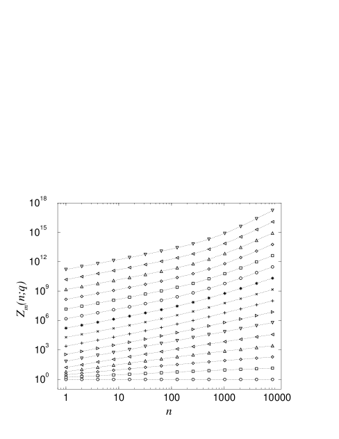
FIG. 5.: Partition functions $Z_{m}(n;q)$ for $q=0.0$ - $3.0$ at intervals of $0.2$. The bottom line corresponds to $q=0.0$, and the top one to $q=3.0$.

In Fig. 5, we display the partition functions $Z_{m}(n;q)$ for several values of $q$ for the one-sided case in a log-log scale. As can be seen from the figure, each partition function exhibits power-law dependence on $n$ for small $n$. We obtain a similar figure for the partition functions $Z_{h}(n;q)$ for the symmetric case. The corresponding scaling exponents $\zeta(q)$ and $\tau(q)$ are shown in Fig. 6. Each curve exhibits strong non-linear dependence on $q$; it is linear for small $q$ and constant for large $q$. Thus, the sequences generated by truncated Lévy flights clearly possess multi-scaling properties.

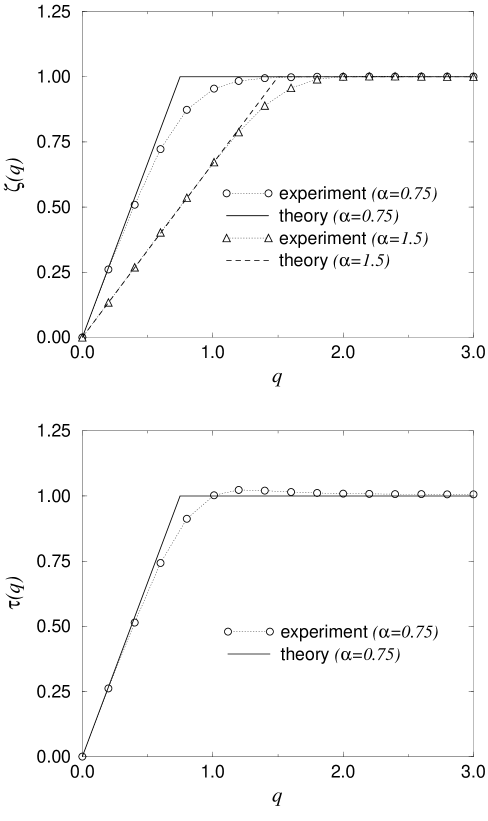
FIG. 6.: Multi-scaling exponents $\zeta(q)$ and $\tau(q)$ for the symmetric (top) and one-sided (bottom) cases. The cut-off parameter $\lambda$ is set at $0.00001$.

V Derivation of the scaling exponents

Now let us derive the scaling exponents $\zeta(q)$ and $\tau(q)$ from the characteristic function Eq. (7). It is clear from the definition of the partition functions that they can be calculated once we know the probability distribution of the sum of random variables $z(n):=\sum_{j=1}^{n}x(j)$. Since the jumps are independent from each other, the probability distribution of $z(n)$ is given by a $n$-times convolution of the truncated Lévy distribution $P_{TL}(x;\lambda)$, i.e., by $P_{TL}^{n}(x;\lambda)$.

As we explained previously, $P_{TL}^{n}(x;\lambda)$ can easily be obtained from the original $P_{TL}(x;\lambda)$ by scaling $x$ and $\lambda$. Making use of this fact, the $q$-th absolute moment $\langle z(n)^{q}\rangle$ of $z(n)$ can be calculated as

$$\langle z(n)^{q}\rangle_{\lambda} = A\int_{0}^{\infty}z^{q}P_{TL}^{n}(z;\lambda)dz=A\int_{0}^{\infty}z^{q}n^{-1/{\alpha}}P_{TL}(n^{-1/{\alpha}}z;n^{1/{\alpha}}\lambda)dz$$ (11)

$$= n^{q/\alpha}A\int_{0}^{\infty}z^{q}P_{TL}(z;n^{1/{\alpha}}\lambda)dz=n^{q/\alpha}\langle z(1)^{q}\rangle_{n^{1/{\alpha}}\lambda},$$ (13)

where the constant $A$ is $2$ for the symmetric case and $1$ for the one-sided case. Here we explicitly indicated the parameter $\lambda$ of the distribution $P_{TL}(x;\lambda)$ as the subscript of the average. Note that if $\langle z(1)^{q}\rangle_{\lambda}$ does not depend on $\lambda$, the scaling exponent is simply given by a linear function $q/\alpha$, and the process does not exhibit multi-scaling. This is the case for the ordinary Lévy stable distribution.

Thus, all we need to calculate is the moment $\langle z(1)^{q}\rangle_{\lambda}$. However, of course, an analytical expression for $P_{TL}(x;\lambda)$ is not attainable except a few specific cases. Here we adopt an approximation which utilizes the facts that the truncated Lévy distribution is different from the ordinary Lévy stable distribution only in the tail part, and that it has a power-law decaying part with an exponent $-1-\alpha$ in the middle (see Figs. 1 and 2). Therefore, it is expected that the moment whose degree $q$ is lower than $\alpha$ is almost the same as that obtained from the ordinary Lévy stable distribution, and the moment for $q>\alpha$ is mostly determined by the asymptotic tail of the truncated Lévy distribution. Note that the moment for $q>\alpha$ does not exist for the ordinary Lévy stable distribution.

(i) Lower moments ($0<q<\alpha$).

We can approximate $P_{TL}(x;\lambda)$ by $P_{L}(x)$ in this case, since they are different only in their tail parts, which does not contribute to the moments lower than $\alpha$ significantly. Therefore, $\langle z(1)^{q}\rangle_{\lambda}$ does not depend on $\lambda$ approximately, and we obtain $\langle z(n)^{q}\rangle\simeq const.\ n^{q/{\alpha}}$. Thus, the scaling exponents $\zeta(q)$ and $\tau(q)$ are given by $q/{\alpha}$ for $0<q<\alpha$. The broken self-similarity of the distribution is not important in this regime.

(ii) Higher moments ($q>\alpha$).

Since the tail of the distribution mainly contributes to the higher moments, we can calculate $\langle z(1)^{q}\rangle_{\lambda}$ approximately if we know the asymptotic form of the distribution. For this purpose, we expand the characteristic function as in the case of the series expansion of ordinary Lévy stable distribution[1]. By expanding the integrand, the truncated Lévy distribution can be expressed as

$$P_{TL}(x;\lambda) = e^{-C\Gamma(-\alpha)\lambda^{\alpha}}\frac{1}{2\pi}\int_{-\infty}^{\infty}\exp\left[C\Gamma(-\alpha)\left\{q(\lambda+i\zeta)^{\alpha}+p(\lambda-i\zeta)^{\alpha}\right\}\right]e^{-i\zeta x}d\zeta$$ (14)

$$= Re\frac{-i}{\pi x}e^{-C\Gamma(-\alpha)\lambda^{\alpha}}\sum_{k=0}^{\infty}\frac{1}{k!}\left\{C\Gamma(-\alpha)\lambda^{\alpha}\right\}^{k}\int_{0}^{\infty}\left[q\left(1+\frac{z}{\lambda x}\right)^{\alpha}+p\left(1-\frac{z}{\lambda x}\right)^{\alpha}\right]^{k}e^{-z}dz\;\;\;\;\;\;\;\;$$ (15)

for the case $0<\alpha<1$. At the lowest order ($k=1$), we recover the original distribution of the increments:

$$P_{TL}(x;\lambda)\sim e^{-C\Gamma(-\alpha)\lambda^{\alpha}}Cpx^{-1-\alpha}e^{-\lambda x}\;\;\;\;(x\gg 1).$$ (16)

With this approximation, the moment $\langle z(1)^{q}\rangle_{\lambda}$ is calculated as

$$\langle z(1)^{q}\rangle_{\lambda}\simeq e^{-C\Gamma(-\alpha)\lambda^{\alpha}}Cp\int_{0}^{\infty}z^{q-1-\alpha}e^{-\lambda z}dz=e^{-C\Gamma(-\alpha)\lambda^{\alpha}}Cp\Gamma(1+q)\lambda^{-q+\alpha},$$ (17)

and we obtain

$$\langle z(n)^{q}\rangle_{\lambda}=n^{q/\alpha}\langle z(1)^{q}\rangle_{n^{1/{\alpha}}\lambda}\sim n^{q/\alpha}\left(n^{1/{\alpha}}\lambda\right)^{-q+\alpha}\sim n^{1}.$$ (18)

Thus, the scaling exponents $\zeta(q)$ and $\tau(q)$ are given by $1$ for $q>\alpha$.

In summary, we approximately derived the following expression for the multi-scaling exponents $\zeta(q)$ and $\tau(q)$:

$$\zeta(q),\tau(q)=\left\{\begin{array}[]{cc}q/{\alpha}&\;\;\;\;(0<q<\alpha),\cr\cr 1&\;\;\;\;(q>\alpha).\end{array}\right.$$ (19)

Note that the above approximation becomes more and more accurate as we extend the power-law decaying part by decreasing $\lambda$, and this result is exact in the asymptotic limit. In Fig. 6, these theoretical curves are compared with the experimental results. Except for small deviations near the transition points, the theoretical results well reproduce the experimental results. Although our estimation here is done for the case $0<\alpha<1$, the theoretical result Eq. (19) seems to be also applicable for $1<\alpha<2$. This type of simple multi-scaling is sometimes called “bi-fractality” and is known, for example, in randomly forced Burgers’ equation[10].

VI Discussion

We analyzed the multi-scaling properties of the truncated Lévy flights based on the smooth truncation introduced by Koponen. As Dubrulle and Laval claimed, truncation is essential for the multi-scaling properties to appear. We clarified this fact and derived the functional form of the scaling exponents for both symmetric and one-sided cases.

As we mentioned previously, the cut-off parameter $\lambda$ may represent the finiteness of the system under consideration. Then it would be natural to assume $\lambda$ as a decreasing function of the system size $L$, for example $\lambda=L^{-1}$, and we can think of the system-size dependence of the truncated Lévy flight. Of course, distribution functions $P_{TL}$ for different system sizes cannot be collapsed simply by rescaling $x$, i.e., finite-size scaling does not hold. However, approximate finite-size scaling relations still hold separately, if we divide $P_{TL}$ into two parts at the power-law decaying part, i.e., into the self-similar part and the tail part. As we explained, the self-similar part is insensitive to $\lambda=L^{-1}$, and $P_{TL}$ for different system sizes collapse to a single curve in this region without rescaling. On the other hand, the tail part is asymptotically given by $P_{TL}(x;L^{-1})\sim x^{-1-\alpha}e^{-x/L}$, which can be rescaled as $L^{1+\alpha}P_{TL}(xL;L^{-1})$ to give a universal curve. Thus, we have two different approximate finite-size scaling relations in different regions of $x$, which is separated by the power-law decaying part. Of course, this is closely related to the bi-fractal behavior of the scaling exponents. Similar asymptotic finite-size scaling is also reported in the sandpile models of self-organized criticality[13].

Recently, Chechkin and Gonchar[14] discussed the finite sample number effect on the scaling properties of a stable Lévy process. (They treated only the symmetric case using a different argument from ours, which was more qualitative and therefore more general in a sense.) They claimed that, due to the finite sample number effect, “spurious” multi-affinity is observed in the numerical simulation and derived the “spurious” multi-scaling exponent. Interestingly, or in some sense obviously, their “spurious” multi-scaling exponent is the same as our multi-scaling exponent, since the truncation of the power-law by $\lambda$ can also be interpreted as mimicking the finite sample number effect of experiments.

Our calculation presented in this paper is similar to our previous work[15] on the multi-scaling properties of the amplitude and difference fields of anomalous spatio-temporal chaos found in systems of non-locally coupled oscillators. The distribution treated there was not the truncated Lévy type but had a form like $(1+x^{2})^{\alpha/2}e^{-\lambda|x|}$. Since this form is easily generated by a simple multiplicative stochastic process, some attempts have been made to model the economic activity using this type of distribution[16, 17].

The bi-fractal behavior of the scaling exponent is the simplest case of multi-scaling, while experimentally observed scaling exponents usually exhibit more complex behavior. Actually, it has long been discussed in the context of fluid turbulence what the shape of the distribution should be to reproduce the experimentally observed scaling exponent[10, 11, 18]. In order to reproduce the behavior of the scaling exponent more realistically in the framework of the truncated Lévy flights discussed here, introduction of correlations to the random variables will be necessary. Studies in this direction are expected.

- [1] W. Feller, An Introduction to Probability Theory and Its Applications vol.II (John Wiley & Sons, Inc., New York, 1971).
- [2] M. F. Shlesinger, G. M. Zaslavsky, and U. Frisch(Eds.), Lévy Flights and Related Topics In Physics (Springer, Berlin, 1995).
- [3] R. N. Mantegna and H. E. Stanley, Phys. Rev. Lett. 73 (1994), 2946.
- [4] I. Koponen, Phys. Rev. E 52 (1995), 1197.
- [5] B. Dubrulle and J. -Ph. Laval, Eur. Phys. J. B 4 (1998), 143.
- [6] R. Cont, M. Potters, and J-P. Bouchaud, cond-mat/9705087.
- [7] J-P. Bouchaud and M. Potters, cond-mat/9905413.
- [8] N. Vandewalle and M. Ausloos, Eur. Phys. J. B 4 (1998), 257.
- [9] K. Ivanova and M. Ausloos, Eur. Phys. J. B 8 (1999), 665.
- [10] U. Frisch, Turbulence, the legacy of A. N. Kolmogorov (Cambridge University Press, Cambridge, 1995).
- [11] T. Bohr, M. H. Jensen, G. Paladin, and A. Vulpiani, Dynamical Systems Approach to Turbulence (Cambridge University Press, Cambridge, 1998).
- [12] H. Bergström, Arkiv För Matematik 2 1952, 375.
- [13] A. Chessa, H. E. Stanley, A. Vespignani, and S. Zapperi, Phys. Rev. E. 59 (1999), 12.
- [14] A. V. Chechkin and V. Yu. Gonchar, cond-mat/9907234.
- [15] H. Nakao and Y. Kuramoto, Eur. Phys. J. B 10 (1999), 345.
- [16] A-H. Sato and H. Takayasu, Physica A 250 (1998), 231.
- [17] D. Sornette, Physica A 250 (1998), 295.
- [18] R. Benzi, L. Biferale, G. Paladin, A. Vulpiani, and M. Vergassola, Phys. Rev. Lett. 67 (1991), 2299.