Thermodynamically consistent mesoscopic fluid particle models for a van der Waals fluid

Abstract

The GENERIC structure allows for a unified treatment of different discrete models of hydrodynamics. We first propose a finite volume Lagrangian discretization of the continuum equations of hydrodynamics through the Voronoi tessellation. We then show that a slight modification of these discrete equations has the GENERIC structure. The GENERIC structure ensures thermodynamic consistency and allows for the introduction of correct thermal noise. In this way, we obtain a consistent discrete model for Lagrangian fluctuating hydrodynamics. For completeness, we also present the GENERIC versions of the Smoothed Particle Dynamics model and of the Dissipative Particle Dynamics model. The thermodynamic consistency endorsed by the GENERIC framework allows for a coherent discussion of the gas-liquid phase coexistence of a van der Waals fluid.

I Introduction

The behaviour of complex fluids like colloids, emulsions, polymers or multiphasic fluids is affected by the strong coupling between the microstructure of these fluids with the macroscopic flow. The complexity of these systems requires the use of novel computer simulations techniques and algorithms. Usual macroscopic approaches that solve partial differential equations with constitutive equations are not very useful because the basic input, the constitutive equation is usually not known. Also, these approaches neglect the presence of thermal noise, which is the responsible for the Brownian motion of small suspended objects and, therefore, for the diffusive processes that affect the microstructure of the fluid. In recent years, there has been a large effort in order to develop mesoscopic techniques in order to tackle the problems arising in the simulation of complex fluids.

Dissipative Particle Dynamics is a mesoscopic particle based simulation method that allows one to model hydrodynamic behavior and that it consistently includes thermal fluctuations. It was introduced by Hoogerbrugge and Koelman in 1991 under the motivation of designing an off-lattice algorithm inspired by the ideas behind the lattice-gas method [1]. Since then, the model has received a great deal of attention. From a theoretical point of view, the model has been given a solid background as a statistical mechanics model [2]. The hydrodynamic behavior has been analyzed [2, 3] and the methods of kinetic theory have provided explicit formulae for the transport coefficients in terms of the model parameters [4]. A generalization of DPD has also been presented in order to conserve energy [5]. From the side of applications, the method is very versatile and has proven to be useful in the simulation of flows in porous media [6], colloidal suspensions [6, 7], polymer suspensions [8], microphase separation of copolymers [9], multicomponent flows [10] and thin-film evolution [11].

The physical picture behind the dissipative particles used in the model is that they represent mesoscopic portions of real fluid, say clusters of molecules moving in a coherent and hydrodynamic fashion. The interaction between these particles are postulated from simplicity and symmetry principles that ensure the correct hydrodynamic behavior. DPD faces, however, a conceptual problem. The thermodynamic behavior of the model is determined by the conservative forces introduced in the model. This forces are assumed to be soft forces in counter distinction to the singular forces of the Lennard-Jones type used in molecular dynamics. But there is no well-defined procedure to relate the shape and amplitude of the conservative forces with a prescribed thermodynamic behavior (although attempts in that direction have been undertaken, see Ref. [9]). Also, it is not clear which physical time and length scales the model actually describes, even though the presence of thermal noise suggests the foggy area of the mesoscopic realm. We will see that both problems are closely related.

Dissipative Particle Dynamics is very similar in spirit to the popular method of Smoothed Particle Dynamics [3]. The method was introduced in the context of astrophysics computation in the early 70’s [12] and very recently it has been applied to the study of laboratory scale viscous [13] and thermal flows [14] in simple geometries. SPD is essentially a Lagrangian discretization of the Navier-Stokes equations by means of a weight function. The procedure transforms the partial differential equations of continuum hydrodynamics into ordinary differential equations. These equations can be further interpreted as the equations of motion for a set of particles interacting with prescribed laws of force. The technique thus allows one to solve PDE’s with molecular dynamics codes. Again, these particles can be understood as physical portions of the fluid that evolve coherently along the flow. The problem with Smoothed Particle Hydrodynamics is that it does not include thermal fluctuations and, therefore, cannot be applied to the study of complex fluids at mesoscopic scales.

We have recently shown that the conceptual problems in DPD and the inclusion of thermal fluctuations in SPD can be resolved by formulating convenient generalizations of both methods under the general framework of GENERIC [15]. In the present paper, we take a further look at the problem of formulating consistent models for the simulation of hydrodynamic problems. Our point of view here is to construct a finite volume algorithm for solving the Navier-Stokes equations in such a way that thermodynamic consistency is retained: The resulting algorithm conserves mass, momentum, and energy, and the entropy is an increasing function of time. Most important, we show how to include thermal noise in a consistent way, this is, producing the Einstein distribution function. We end up, therefore, with an algorithm for simulating fluctuating hydrodynamics in a Lagrangian way [16]. This algorithm can be used as the basis for simulating colloidal suspensions, where the Brownian motion of the colloidal particles is due to the thermal fluctuations on the solvent [17]. We show also another potential application to multiphasic flow of the gas-liquid type. When the fluid is described with a van der Waals equation of state, the Einstein equilibrium distribution allows to discuss the gas-liquid phase transition in probabilistic terms. Such probabilistic approaches to equilibrium phase transitions have been studied in the past [18]. We should note, however, that the GENERIC finite volume algorithm should allow us to study fully non-equilibrium situations created by external boundary conditions that can drive the system out of equilibrium. Start up of boiling of water in a pot could be addressed with the proposed GENERIC finite volume algorithm.

Other very recent approaches to the study of the flow of liquid-vapor coexisting fluids are the Lattice Boltzmann model introduced by Swift, Osborn and Yeomans [19] and improved in Refs. [20] in order to have a thermodynamically consistent model for a dense fluid that may exhibit liquid-vapor coexistence. However, only isothermal models have been considered up to now. A second very promising approach is the Direct Simulation Monte Carlo method [21] that has been conveniently generalized to deal with dense liquids with liquid-vapor coexistence [22].

In order to construct the finite volume algorithm we have been strongly inspired by the work of Flekkoy and Coveney [23]. In that paper, the authors present a “bottom-up” derivation of Dissipative Particle Dynamics. Physical space is divided into Voronoi cells and explicit definitions for the mass, momentum and energy of the cells in terms of the microscopic degrees of freedom (positions and momenta of the constituent molecules of the fluid) are given. The time derivatives of these phase functions have the structure of “microscopic balance equations” in a discrete form. These equations are then divided into “average” and “stochastic” parts. To further advance into the formulation of a practical algorithm, the authors then propose phenomenological, physically sensible, expressions for the average part and require the fulfillment of the fluctuation-dissipation theorem for the stochastic part. Because of the use of the phenomenological expressions, we cannot consider this a “bottom-up” approach. Strictly speaking, a bottom-up approach would require the use of a projection operator technique or kinetic theory, in order to relate the transport coefficients with the microscopic dynamics of the system (in the form of Green-Kubo formulae, for example).

Instead, we propose in this paper a conspicuous “top-down” approach in which the deterministic continuum equations of hydrodynamics are the starting point. By making intensive use of the smooth Voronoi tessellation discovered by Flekkoy and Coveney the form of the discrete equations is dictated by the very structure of the continuum equations. Our approach is similar to that in Ref. [24]. However, we make a further requirement on the resulting finite volume discretization, which is that they must have the GENERIC structure. This enforces the addition of a tiny bit into the momentum equation. Having the GENERIC structure, it is trivial to obtain the stochastic part, which will be given by the fluctuation-dissipation theorem. In the concluding section we will show the similarities and differences between our equations and those derived by Flekkoy and Coveney.

The approach presented in this work has also a strong resemblance with Yuan and Doi simulation method which also uses the Voronoi tessellation in Lagrangian form [25] (see also [26]). They have applied the method to the simulation of concentrated emulsions under flow and several other applications to complex fluids are mentioned. The main difference between our work and that of Ref. [25] is the special care we have taken in order to have thermodynamic consistency through the GENERIC formalism. This allows, among other things, to include correct thermal noise and describe diffusive aspects produced by Brownian motion on mesoscopic objects. Another difference is that we deal with a compressible fluid in which the pressure is given through the equation of state as a function of mass and entropy densities, in counterdistinction with Ref. [25] where the pressure is obtained by satisfying the incompressibility condition. Compressibility is necessary if gas-liquid coexistence is to be described.

II Review of GENERIC

For the sake of completeness we review in this section the GENERIC formalism developed by Öttinger and Grmela [28]. The formalism of GENERIC (acronym for General Equation for Non Equilibrium Reversible Irreversible Coupling) states that all physically sounded transport equations in non-equilibrium thermodynamics have the same structure. A large body of evidence confirms this assertion: Linear irreversible thermodynamics, non-relativistic and relativistic hydrodynamics, Boltzmann’s equation, polymer kinetic theory, and chemical reactions, just to mention a few, have all the GENERIC structure [28, 29]. The GENERIC formalism is not only a way of rewriting known transport equations in a physically transparent way, but it allows us to derive dynamical equations for new systems not considered so far in an astonishing simple way. The very structure of the formalism ensures thermodynamic consistency, energy conservation and positive entropy production.

The essential assumption on which GENERIC is founded is that the relevant variables $x$ used to describe the system at a certain level of description evolve in a time scale well-separated from the time scales of other variables in the system. In other words, the variables should provide a closed description in which the present state of the system depends only on the very recent past and memory effects can be neglected. This is a recurrent theme in non-equilibrium statistical mechanics since the pioneering works of Zwanzig and Mori [27]. Actually, the GENERIC structure can be deduced from first principles by using standard projection operator formalism under a Markovian approximation [28].

Two basic building blocks in the GENERIC formalism are the energy $E(x)$ and entropy $S(x)$ functions of the variables $x$ describing the state of the system at a particular level of description [28]. The GENERIC dynamic equations are given then by

$$\frac{dx}{dt}=L\!\cdot\!\frac{\partial E}{\partial x}+M\!\cdot\!\frac{\partial S}{\partial x}.$$ (1)

The first term in the right hand side is named the reversible part of the dynamics and the second term is named the irreversible part. The predictive power of GENERIC relies in the fact that very strong requirements exists on the matrices $L,M$ leaving small room for the physical input about the system. First, $L$ is antisymmetric whereas $M$ is symmetric and positive semidefinite. Most important, the following degeneracy conditions should hold

$$L\!\cdot\!\frac{\partial S}{\partial x}=0,\quad\quad\quad M\!\cdot\!\frac{\partial E}{\partial x}=0.$$ (2)

These properties ensure that the energy is a dynamical invariant, $\dot{E}=0$, and that the entropy is a non-decreasing function of time, $\dot{S}\geq 0$, as can be proved by a simple application of the chain rule and the equations of motion (1). In the case that other dynamical invariants $I(x)$ exist in the system (as, for example, linear or angular momentum), then further conditions must be satisfied by $L,M$. In particular,

$$\frac{\partial I}{\partial x}\!\cdot\!L\!\cdot\!\frac{\partial E}{\partial x}=0,\quad\quad\quad\frac{\partial I}{\partial x}\!\cdot\!M\!\cdot\!\frac{\partial S}{\partial x}=0.$$ (3)

which ensure that $\dot{I}=0$.

The deterministic equations (1) are, actually, an approximation in which thermal fluctuations are neglected. If thermal fluctuations are not neglected, the dynamics is described by stochastic differential equations or, equivalently, by a Fokker-Planck equation that governs the probability distribution function $\rho=\rho(x,t)$. This FPE has the form [28]

$$\partial_{t}\rho=-\frac{\partial}{\partial x}\!\cdot\!\left[\rho\left[L\!\cdot\!\frac{\partial E}{\partial x}+M\!\cdot\!\frac{\partial S}{\partial x}\right]-k_{B}M\!\cdot\!\frac{\partial\rho}{\partial x}\right],$$ (4)

where $k_{B}$ is Boltzmann’s constant.

The distribution function of the variables of a given system at equilibrium is given by the Einstein distribution function. This assertion can be proved under quite general hypothesis on the mixing character of the microscopic dynamics of the system [30]. If the microscopic dynamics ensures the existence of dynamical invariants like the energy $E(x)$ and, perhaps, other invariants $I(x)$, then the Einstein distribution function takes the form [30]

$$\rho^{\rm eq}(x)=g(E(x),I(x))\exp\{S(x)/k_{B}\},$$ (5)

where the function $g$ is completely determined by the arbitrary initial distribution of dynamical invariants. For example, if at an initial time the value of the invariants $E(x),I(x)$ are known with high precision to be $E_{0},I_{0}$, then the Einstein distribution function takes the form

$$\rho^{\rm eq}(x)=\frac{\delta(E(x)-E_{0})\delta(I(x)-I_{0})}{\Omega(E_{0},I_{0})}\exp\{k_{B}^{-1}S(x)\},$$ (6)

where $\Omega(E_{0},I_{0})$ is the normalization. Given the general argument behind the Einstein distribution function [30], it is sensible to demand that the Fokker-Planck equation (4) has as its (unique) equilibrium distribution function the Einstein distribution. This can be achieved, actually, if the following further conditions on the form of the matrices $L,M$ hold,

$$\frac{\partial}{\partial x}\!\cdot\!\left[L\!\cdot\!\frac{\partial E}{\partial x}\right]=0,\quad\quad\quad M\!\cdot\!\frac{\partial I}{\partial x}=0.$$ (7)

The first property can be derived independently with projection operator techniques [28] whereas the second property implies that the last equation in (3) is automatically satisfied.

When fluctuations are present, the entropy function $S(x)$ might be a decreasing function of time. However, if one considers the entropy functional

$${\cal S}[\rho_{t}]=\int S(x)\rho(x,t)dx-k_{B}\int\rho(x,t)\ln\rho(x,t)dx,$$ (8)

it is possible to prove by using the Fokker-Planck equation (4) that $\partial_{t}{\cal S}[\rho_{t}]\geq 0$. In other words, the entropy functional plays the role of a Lyapunov function.

The stochastic differential equations that are mathematically equivalent to the above Fokker-Planck equation are given, with Itô interpretation, by [31]

$$dx=\left[L\!\cdot\!\frac{\partial E}{\partial x}+M\!\cdot\!\frac{\partial S}{\partial x}+k_{B}\frac{\partial}{\partial x}\!\cdot\!M\right]dt+d\tilde{x},$$ (9)

to be compared with the deterministic equations (1). The stochastic term $d\tilde{x}$ in Eqn. (9) is a linear combination of independent increments of the Wiener process. It satisfies the mnemotechnical Itô rule

$$d\tilde{x}d\tilde{x}^{T}=2k_{B}Mdt,$$ (10)

which means that $d\tilde{x}$ is an infinitesimal of order $1/2$ [31]. Eqn. (10) is a compact and formal statement of the fluctuation-dissipation theorem.

When formulating new models it might be convenient to specify $d\tilde{x}$ directly instead of $M$. This ensures that $M$ through (10) automatically satisfies the symmetry and positive definite character. In order to guarantee that the total energy and dynamical invariants do not change in time, a strong requirement on the form of $d\tilde{x}$ holds,

$$\frac{\partial E}{\partial x}\!\cdot\!d\tilde{x}=0,\quad\quad\frac{\partial I}{\partial x}\!\cdot\!d\tilde{x}=0,$$ (11)

implying the last equations in (2) and (7). The geometrical meaning of (11) is clear. The random kicks produced by $d\tilde{x}$ on the state $x$ are orthogonal to the gradients of $E,I$. These gradients are perpendicular vectors (strictly speaking they are one forms) to the hypersurface $E(x)=E_{0},I(x)=I_{0}$. Therefore, the kicks let the state $x$ always within the hypersurface of dynamical invariants.

We finally close this section by noting that, formally, the size of the fluctuations is governed by the Boltzmann constant $k_{B}$. If we take $k_{B}\rightarrow 0$, the stochastic differential equation (9) becomes the deterministic equations (1) and the Fokker-Planck equation (4) has only first derivatives in the same way as the Liouville equation. In this limit, the distribution function $\rho(x,t)$ does not show dispersion and it is essentially a Dirac delta function evaluated on the solution of the deterministic equation. In this case, the entropy functional ${\cal S}[\rho]$ reduces to the entropy $S(x)$ and the entropy is a non-decreasing function of time.

III Finite volume method with Voronoi cells

As a first step for deriving the GENERIC equations for a model of fluid particles, we consider the method of finite volumes for the numerical integration of the equations of continuum hydrodynamics. The basic motivation for this is to have a set of reference equations that serve as guidelines for the modeling in the GENERIC equations in such a way that we can consider the GENERIC equations as reasonable approximations to the equations of continuum hydrodynamics.

The finite volume method consists on integrating the continuum equations of hydrodynamics in a finite region of space (or finite volume) in such a way that ordinary differential equations for the average fields over the finite regions emerge. In this section we present a finite volume method that uses the Voronoi construction as a conceptually and mathematically elegant method for discretizing the continuum equations of hydrodynamics.

Following Flekkoy and Coveney [23], we introduce the smoothed characteristic function of the Voronoi cell $\mu$

$$\chi_{\mu}({\bf r})=\frac{\Delta(|{\bf r}-{\bf R}_{\mu}|)}{\sum_{\nu}\Delta(|{\bf r}-{\bf R}_{\nu}|)},$$ (12)

where the function $\Delta(r)=\exp\{-r^{2}/2\sigma^{2}\}$ is a Gaussian of width $\sigma$. When $\sigma\rightarrow 0$, the smoothed characteristic function tends to the actual characteristic function of the Voronoi cell, this is

$$\lim_{\sigma\rightarrow 0}\chi_{\mu}({\bf r})=\prod_{\nu}\theta(|{\bf r}-{\bf R}_{\nu}|-|{\bf r}-{\bf R}_{\mu}|),$$ (13)

where $\theta(x)$ is the Heaviside step function. The Voronoi characteristic function (13) takes the value 1 if ${\bf r}$ is nearer to ${\bf R}_{\mu}$ than to any other ${\bf R}_{\nu}$ with $\nu\neq\mu$. Note that the characteristic function produces a covering of all space (i.e., a partition of unity), this is,

$$\sum_{\mu}\chi_{\mu}({\bf r})=1.$$ (14)

We introduce the volume of the Voronoi cell through

$${\cal V}_{\mu}=\int_{V_{T}}d{\bf r}\chi_{\mu}({\bf r}),$$ (15)

which satisfies the closure condition

$$\sum_{\mu}{\cal V}_{\mu}=V_{T},$$ (16)

where $V_{T}$ is the total volume. In Fig. 2 we show the Voronoi tessellation corresponding to 15 particles seeded at random in a periodic box. For an introduction to the Voronoi tessellation see [32].

FIG. 1.: Contour line at $\chi_{\mu}({\bf r})=0.5$ for the set of all characteristic functions of the 15 particles located at random in a periodic box of size $L=100$. The value of $\sigma$ is $0.03$.

FIG. 2.: Contour lines of the function $\chi_{\mu}({\bf r})$ for particle $\mu=1$ of the previous tessellation. Inside the closed region the value of $\chi_{\mu}({\bf r})$ is 1 and outside is zero.

We mention now some other useful properties of the smoothed characteristic function that will be needed later. First, due to the Gaussian form of $\Delta(r)$,

$$\nabla\Delta(r)=-\frac{1}{\sigma^{2}}\Delta(r){\bf r}.$$ (17)

Therefore,

$$\frac{\partial}{\partial{\bf r}}\chi_{\mu}({\bf r}) = -\frac{1}{\sigma^{2}}\chi_{\mu}({\bf r})({\bf r}-{\bf R}_{\mu})$$ (18)

$$+ \frac{1}{\sigma^{2}}\chi_{\mu}({\bf r})\sum_{\nu}\chi_{\nu}({\bf r})({\bf r}-{\bf R}_{\nu}).$$ (19)

By using the following property

$$\chi_{\mu}({\bf r})(1-\chi_{\mu}({\bf r}))=\sum_{\nu\neq\mu}\chi_{\mu}({\bf r})\chi_{\nu}({\bf r}),$$ (20)

which can be proved by using the definition (12), one can rewrite Eqn. (19) as

$$\frac{\partial}{\partial{\bf r}}\chi_{\mu}({\bf r})=\frac{1}{\sigma^{2}}\sum_{\nu}\chi_{\mu}({\bf r})\chi_{\nu}({\bf r})({\bf R}_{\mu}-{\bf R}_{\nu}).$$ (21)

Another useful relation is,

$$\frac{\partial}{\partial{\bf R}_{\nu}}\chi_{\mu}({\bf r}) = \delta_{\mu\nu}\frac{1}{\sigma^{2}}\chi_{\mu}({\bf r})({\bf r}-{\bf R}_{\mu})$$ (22)

$$- \frac{1}{\sigma^{2}}\chi_{\mu}({\bf r})\chi_{\nu}({\bf r})({\bf r}-{\bf R}_{\nu}).$$ (23)

We now introduce the following two quantities

$$A_{\mu\nu} \equiv R_{\mu\nu}\int\frac{d{\bf r}}{\sigma^{2}}\chi_{\mu}({\bf r})\chi_{\nu}({\bf r}),$$ (24)

$${\bf c}_{\mu\nu} \equiv \frac{R_{\mu\nu}}{A_{\mu\nu}}\int\frac{d{\bf r}}{\sigma^{2}}\chi_{\mu}({\bf r})\chi_{\nu}({\bf r})\left({\bf r}-\frac{{\bf R}_{\mu}+{\bf R}_{\nu}}{2}\right),$$ (25)

where $R_{\mu\nu}=|{\bf R}_{\mu}-{\bf R}_{\nu}|$. In appendix X we show that in the limit $\sigma\rightarrow 0$ the quantity $A_{\mu\nu}$ is actually the area of the contact face $\mu\nu$ between Voronoi cells $\mu$ and $\nu$, whereas the vector ${\bf c}_{\mu\nu}$ is the position of the center of mass of the face $\mu\nu$ with respect to the “center” of the face $({\bf R}_{\mu}+{\bf R}_{\nu})/2$.

A Balance equations

We introduce now the cell average ${[\phi]}_{\mu}(t)$ over the Voronoi cell $\mu$ of an arbitrary density field $\phi({\bf r},t)$

$${[\phi]}_{\mu}(t)=\frac{1}{{\cal V}_{\mu}}\int d{\bf r}\phi({\bf r},t)\chi_{\mu}({\bf r}).$$ (26)

We will refer to ${[\phi]}_{\mu}(t)$ as a cell variable and we will see that it is an approximation for the value of the field at the discrete points given by the cell centers.

In principle, the Voronoi cell centers are allowed to move in an arbitrary way, this is, ${\bf R}_{\mu}(t)$ are prescribed functions of time. The time derivative of the cell averages is given by

$$\frac{d}{dt}{[\phi]}_{\mu}(t) = -\frac{\dot{\cal V}_{\mu}}{{\cal V}_{\mu}}{[\phi]}_{\mu}(t)$$ (27)

$$+ \frac{1}{{\cal V}_{\mu}}\int d{\bf r}\phi({\bf r},t)\frac{d}{dt}\chi_{\mu}({\bf r})$$ (28)

$$+ \frac{1}{{\cal V}_{\mu}}\int d{\bf r}\chi_{\mu}(t)\partial_{t}\phi({\bf r},t),$$ (29)

where the dot means the time derivative. We see that ${[\phi]}_{\mu}(t)$ changes due to both, the motion of the cells and the intrinsic dependence of the field $\phi({\bf r},t)$ on time.

Now, we will assume that the field $\phi({\bf r},t)$ obeys a balance equation, this is

$$\partial_{t}\phi({\bf r},t)=-\nabla\!\cdot\!{\bf J}({\bf r},t),$$ (30)

where ${\bf J}({\bf r},t)$ is an appropriate current density. By integration by parts of the nabla operator and use of Eqns. (21) and (20) one arrives easily at the following expression

$$\frac{d}{dt}{[\phi]}_{\mu}(t) = -\frac{\dot{\cal V}_{\mu}(t)}{{\cal V}_{\mu}}{[\phi]}_{\mu}(t)$$ (31)

$$+ \frac{1}{{\cal V}_{\mu}}\sum_{\nu}A_{\mu\nu}{\bf e}_{\mu\nu}\!\cdot\!\left([{\bf J}]_{\mu\nu}-[\phi]_{\mu\nu}\frac{\dot{{\bf R}}_{\mu}+\dot{{\bf R}}_{\nu}}{2}\right)$$ (32)

$$+ \frac{1}{{\cal V}_{\mu}}\sum_{\nu}\frac{A_{\mu\nu}}{R_{\mu\nu}}[\mbox{\boldmath$\phi$}]^{||}_{\mu\nu}\!\cdot\!\dot{{\bf R}}_{\mu\nu},$$ (33)

where

$${\bf e}_{\mu\nu} = \frac{{\bf R}_{\mu\nu}}{R_{\mu\nu}},$$ (34)

$${\bf R}_{\mu\nu} = {\bf R}_{\mu}-{\bf R}_{\nu},$$ (35)

$$R_{\mu\nu} = |{\bf R}_{\mu}-{\bf R}_{\nu}|,$$ (36)

and we have introduced the face averages

$$[\cdots]_{\mu\nu} = \frac{R_{\mu\nu}}{A_{\mu\nu}}\int\frac{d{\bf r}}{\sigma^{2}}\chi_{\mu}({\bf r})\chi_{\nu}({\bf r})\cdots$$ (37)

$${[\cdots]}_{\mu\nu}^{||} = \frac{R_{\mu\nu}}{A_{\mu\nu}}\int\frac{d{\bf r}}{\sigma^{2}}\chi_{\mu}({\bf r})\chi_{\nu}({\bf r})\left({\bf r}-\frac{{\bf R}_{\nu}+{\bf R}_{\mu}}{2}\right)\cdots$$ (38)

Note that in the limit of sharp boundaries $\sigma\rightarrow 0$, $\mbox{\boldmath$\phi$}^{||}_{\mu\nu}$ is a vector which is parallel to the face $\mu\nu$, whereas ${\bf e}_{\mu\nu}$ is perpendicular to the face.

We can write Eqn. (33) in the form

$$\frac{d}{dt}\left({\cal V}_{\mu}{[\phi]}_{\mu}\right) = \sum_{\nu}A_{\mu\nu}{\bf e}_{\mu\nu}\left([{\bf J}]_{\mu\nu}-[\phi]_{\mu\nu}\frac{\dot{{\bf R}}_{\mu}+\dot{{\bf R}}_{\nu}}{2}\right)$$ (39)

$$+ \sum_{\nu}\frac{A_{\mu\nu}}{R_{\mu\nu}}[\mbox{\boldmath$\phi$}]^{||}_{\mu\nu}\!\cdot\!\dot{\bf R}_{\mu\nu},$$ (40)

which satisfies

$$\frac{d}{dt}\left(\sum_{\mu}{\cal V}_{\mu}{[\phi]}_{\mu}\right)=0,$$ (41)

due to the symmetries $[\cdots]_{\mu\nu}=[\cdots]_{\nu\mu}$, $[\cdots]^{||}_{\mu\nu}=[\cdots]^{||}_{\nu\mu}$ of the face averages. Equation (41) shows that the Voronoi discretization of the balance equation (30) conserves exactly the extensive variables (which are of the form density$\times$volume).

B Finite volumes for an inviscid fluid

In what follows we will apply the method of finite volumes to the continuum equations of hydrodynamics. For the sake of clarity, we first consider the reversible part of the equations, which correspond the the usual Euler equations for an inviscid fluid. In the next subsection we consider the irreversible part.

The Euler equations for an inviscid fluid are the continuity equation

$$\partial_{t}\rho({\bf r},t)=-\nabla\!\cdot\!{\bf g}({\bf r},t),$$ (42)

the momentum balance equation

$$\partial_{t}{\bf g}({\bf r},t)=-\nabla P({\bf r},t)-\nabla\!\cdot\!{\bf g}({\bf r},t){\bf v}({\bf r},t),$$ (43)

and the entropy equation

$$\partial_{t}s({\bf r},t)=-\nabla\!\cdot\!s({\bf r},t){\bf v}({\bf r},t).$$ (44)

In these equations, $\rho({\bf r},t)$ is the mass density field, ${\bf g}({\bf r},t)=\rho({\bf r},t){\bf v}({\bf r},t)$ is the momentum density field, with ${\bf v}({\bf r},t)$ the velocity field, and $s({\bf r},t)$ is the entropy density field (entropy per unit volume). The pressure field $P({\bf r},t)$ is given, according to the local equilibrium assumption, by $P({\bf r},t)=P^{\rm eq}(\rho({\bf r},t),s({\bf r},t))$ where $P^{\rm eq}(\rho,s)$ is the equilibrium equation of state that gives the macroscopic pressure in terms of the mass and entropy densities.

We now write Eqn. (40) for the case that $\phi=\rho$. If the Voronoi cells do not move, then $\dot{{\bf R}}_{\mu}=0$ and expression (40) simplifies considerably,

$$\frac{d}{dt}M_{\mu}(t)=\sum_{\nu}A_{\mu\nu}{\bf e}_{\mu\nu}\!\cdot\![\rho{\bf v}]_{\mu\nu},$$ (45)

where $M_{\mu}={\cal V}_{\mu}{[\rho}]_{\mu}$ is the mass of the Voronoi cell $\mu$. This corresponds to a Eulerian discretization of the continuity equation (42). The physical meaning of Eqn. (45) is clear: $A_{\mu\nu}{\bf e}_{\mu\nu}\!\cdot\![\rho{\bf v}]_{\mu\nu}$ is the total mass per unit time that crosses face $\mu\nu$ and the rate of change of the mass of the cell $\mu$ is the sum of this quantity for each face $\mu\nu$.

The Lagrangian discretization of the continuity equation in Eqn. (42) is obtained by specifying the motion of the cells according to

$$\dot{\bf R}_{\mu}(t)={[{\bf v}]}_{\mu}(t).$$ (46)

In this way, the Voronoi cells “follow” (the best they can) the flow field. We can write Eqn. (40) for the case (42) as

$$\left.\dot{M}_{\mu}\right|_{\rm rev} = \sum_{\nu}A_{\mu\nu}{\bf e}_{\mu\nu}\!\cdot\!\left({[\rho{\bf v}]}_{\mu\nu}-{[\rho]}_{\mu\nu}\frac{{[{\bf v}]}_{\mu}+{[{\bf v}]}_{\nu}}{2}\right)$$ (47)

$$+ \sum_{\nu}\frac{A_{\mu\nu}}{R_{\mu\nu}}{[\rho]}^{||}_{\mu\nu}\!\cdot\!({[{\bf v}]}_{\mu}-{[{\bf v}]}_{\nu}).$$ (48)

The momentum balance equation (43) can similarly be treated and the following Lagrangian finite volume equation arise

$$\left.\dot{\bf P}_{\mu}\right|_{\rm rev} = \sum_{\nu}A_{\mu\nu}{\bf e}_{\mu\nu}{[P]}_{\mu\nu}$$ (51)

$$+\sum_{\nu}A_{\mu\nu}{\bf e}_{\mu\nu}\!\cdot\!\left({[{\bf g}{\bf v}]}_{\mu\nu}-{[{\bf g}]}_{\mu\nu}\frac{{[{\bf v}]}_{\mu}+{[{\bf v}]}_{\nu}}{2}\right)$$

$$+\sum_{\nu}\frac{A_{\mu\nu}}{R_{\mu\nu}}{[{\bf g}]}^{||}_{\mu\nu}\!\cdot\!({[{\bf v}]}_{\mu}-{[{\bf v}]}_{\nu}),$$

where we have introduced the total momentum of cell $\mu$ ${\bf P}_{\mu}={\cal V}_{\mu}{\bf g}_{\mu}$.

Finally, the entropy equation Eqn. (44) takes the following Lagrangian discretization

$$\left.\dot{S}_{\mu}\right|_{\rm rev} = \sum_{\nu}A_{\mu\nu}{\bf e}_{\mu\nu}\!\cdot\!\left({[s{\bf v}]}_{\mu\nu}-{[s]}_{\mu\nu}\frac{{[{\bf v}]}_{\mu}+{[{\bf v}]}_{\nu}}{2}\right)$$ (52)

$$+ \sum_{\nu}\frac{A_{\mu\nu}}{R_{\mu\nu}}{[s]}^{||}_{\mu\nu}\!\cdot\!({[{\bf v}]}_{\mu}-{[{\bf v}]}_{\nu}),$$ (53)

where $S_{\mu}={\cal V}_{\mu}s_{\mu}$ is the total entropy of cell $\mu$.

In all these evolution equations, the subscript $|_{\rm rev}$ denotes that the equations are actually the reversible part of the dynamics of a truly viscous fluid.

C Gradient expansion

The above equations (48), (51), and (53) are rigorous and exact and do not depend on the typical size of the Voronoi cells. By taking sufficiently small cells, we can approximate the equations and transform them into a closed set of equations for the cell variables. In this way, a computationally feasible algorithm can be proposed for the updating of cell variables.

Let us assume that the hydrodynamic fields have a typical length scale of variation $\lambda_{H}$ and that the typical distance between cell centers is $\lambda_{c}$. We introduce the resolution parameter as $r=\lambda_{c}/\lambda_{H}$ and will assume that this parameter is very small. Therefore the dimensionless quantity

$$\frac{\lambda_{c}}{\phi({\bf R}_{\mu})}\nabla\phi({\bf R}_{\mu})\sim r,$$ (54)

will be very small. By denoting with ${\cal O}(\nabla)$ those terms which are of relative size $r$, we can write the cell average as

$${[\phi]}_{\mu} \equiv \frac{1}{{\cal V}_{\mu}}\int d{\bf r}\chi_{\mu}({\bf r})\phi({\bf r})$$ (55)

$$= \frac{1}{{\cal V}_{\mu}}\int d{\bf r}\chi_{\mu}({\bf r})\phi({\bf r}-{\bf R}_{\mu}+{\bf R}_{\mu})$$ (56)

$$= \phi({\bf R}_{\mu})+\frac{1}{{\cal V}_{\mu}}\int d{\bf r}\chi_{\mu}({\bf r})({\bf r}-{\bf R}_{\mu})\!\cdot\!\nabla\phi({\bf R}_{\mu})+{\cal O}(\nabla^{2})$$ (57)

$$= \phi({\bf R}_{\mu})+{\cal O}(\nabla).$$ (58)

Performing similar Taylor expansions we obtain easily

$${[\phi]}_{\mu\nu}=\phi\left(\frac{{\bf R}_{\mu}+{\bf R}_{\nu}}{2}\right)+{\cal O}(\nabla).$$ (59)

Also

$$\phi\left(\frac{{\bf R}_{\mu}+{\bf R}_{\nu}}{2}\right)=\frac{\phi({\bf R}_{\mu})+\phi({\bf R}_{\nu})}{2}+{\cal O}(\nabla^{2}),$$ (60)

and, therefore,

$${[\phi]}_{\mu\nu}=\frac{{[\phi]}_{\mu}+{[\phi]}_{\nu}}{2}+{\cal O}(\nabla).$$ (61)

After some algebra it is easy to show that

$${[\phi\psi]}_{\mu\nu}={[\phi]}_{\mu\nu}{[\psi]}_{\mu\nu}+{\cal O}(\nabla^{2}).$$ (62)

Finally,

$${[{\bf\phi}]}^{||}_{\mu\nu}=\frac{{[\phi]}_{\mu}+{[\phi]}_{\nu}}{2}{\bf c}_{\mu\nu}+{\cal O}(\nabla).$$ (63)

By using these Taylor approximations in Eqns. (48), (51), and (53) we obtain the final Voronoi finite volume discrete equations for the inviscid fluid,

$$\left.\dot{M}_{\mu}\right|_{\rm rev} = \sum_{\nu}\frac{A_{\mu\nu}}{R_{\mu\nu}}\frac{{[\rho]}_{\mu}+{[\rho]}_{\nu}}{2}{\bf c}_{\mu\nu}\!\cdot\!({[{\bf v}]}_{\mu}-{[{\bf v}]}_{\nu}),$$ (64)

$$\left.\dot{\bf P}_{\mu}\right|_{\rm rev} = \sum_{\nu}A_{\mu\nu}{\bf e}_{\mu\nu}\frac{{[P]}_{\mu}+{[P]}_{\nu}}{2}$$ (65)

$$+ \sum_{\nu}\frac{A_{\mu\nu}}{R_{\mu\nu}}\frac{{[\rho]}_{\mu}+{[\rho]}_{\nu}}{2}\frac{{[{\bf v}]}_{\mu}+{[{\bf v}]}_{\nu}}{2}{\bf c}_{\mu\nu}\!\cdot\!({[{\bf v}]}_{\mu}-{[{\bf v}]}_{\nu}),$$ (66)

$$\left.\dot{S}_{\mu}\right|_{\rm rev} = \sum_{\nu}\frac{A_{\mu\nu}}{R_{\mu\nu}}\frac{{[s]}_{\mu}+{[s]}_{\nu}}{2}{\bf c}_{\mu\nu}\!\cdot\!({[{\bf v}]}_{\mu}-{[{\bf v}]}_{\nu}).$$ (67)

These equations become closed equations for $M_{\mu},{\bf P}_{\mu},S_{\mu}$ by using

$${[\rho]}_{\mu} = \frac{M_{\mu}}{{\cal V}_{\mu}},$$ (68)

$${[s]}_{\mu} = \frac{S_{\mu}}{{\cal V}_{\mu}},$$ (69)

$${[P]}_{\mu} = P^{\rm eq}({[\rho]}_{\mu},{[s]}_{\mu}),$$ (70)

where in the last equation for the pressure we have used again a Taylor expansion and neglected terms of order ${\cal O}(\nabla)$.

D Finite volumes for a viscous fluid

Having studied the inviscid fluid, in which there are no dissipative contributions to the motion of the fluid, we turn now to the general viscous fluid. The continuum equations are given by [33]

$$\partial_{t}\rho({\bf r},t) = -\nabla\!\cdot\!\rho({\bf r},t){\bf v}({\bf r},t),$$ (71)

$$\partial_{t}{\bf g}({\bf r},t) = -\nabla P({\bf r},t)-\nabla\!\cdot\!{\bf g}({\bf r},t){\bf v}({\bf r},t)-\nabla\!\cdot\!(\overline{\bf\Pi}+\Pi{\bf 1}),$$ (72)

$$\partial_{t}s({\bf r},t) = -\nabla\!\cdot\!s({\bf r},t){\bf v}({\bf r},t)$$ (73)

$$- \frac{1}{T}\nabla\!\cdot\!{\bf J}^{q}+\frac{2\eta}{T}\overline{\nabla{\bf v}}:\overline{\nabla{\bf v}}+\frac{\zeta}{T}(\nabla\!\cdot\!{\bf v})^{2},$$ (74)

where, by comparison with Eqns. (42), (43), (44) we can recognize the purely irreversible terms in the momentum and entropy equations. Here, $T$ is the temperature field (which, as the pressure, is a function of $\rho,s$ through the local equilibrium assumption). The double dot implies double contraction. These equations have to be supplemented with the constitutive equations for the traceless symmetric part $\overline{\bf\Pi}$ of the viscous stress tensor, the trace $\Pi$ of the viscous stress tensor, and the heat flux ${\bf J}^{q}$. They are

$$\overline{\bf\Pi} = -2\eta\overline{\nabla{\bf v}},$$ (75)

$$\Pi = -\zeta\nabla\!\cdot\!{\bf v},$$ (76)

$${\bf J}^{q} = -\kappa\nabla T=\kappa T^{2}\nabla\frac{1}{T},$$ (77)

where the traceless symmetric part of the velocity gradient tensor is

$$\overline{\nabla{\bf v}}=\frac{1}{2}\left(\nabla{\bf v}+(\nabla{\bf v})^{T}\right)-\frac{1}{D}\nabla\!\cdot\!{\bf v}.$$ (78)

Here, $D$ is the dimension of physical space. In principle, the shear viscosity $\eta$, the bulk viscosity $\zeta$ and the thermal conductivity $\kappa$ might depend on the state of the fluid through $\rho,s$.

Following identical steps as for the inviscid fluid, we see that the viscous (irreversible) term in the momentum balance equation translates into

$$\left.\dot{\bf P}_{\mu}\right|_{\rm irr}=\sum_{\nu}A_{\mu\nu}{\bf e}_{\mu\nu}\!\cdot\![\eta\overline{\nabla{\bf v}}]_{\mu\nu}+\sum_{\nu}A_{\mu\nu}{\bf e}_{\mu\nu}[\zeta\nabla\!\cdot\!{\bf v}]_{\mu\nu}.$$ (79)

We now consider the gradient expansion on each term. For example,

$$\left[\eta\overline{\nabla{\bf v}}\right]_{\mu\nu} = \frac{\left[\eta\overline{\nabla{\bf v}}\right]_{\mu}+\left[\eta\overline{\nabla{\bf v}}\right]_{\nu}}{2}+{\cal O}(\nabla),$$ (80)

$$\left[\zeta\nabla\!\cdot\!{\bf v}\right]_{\mu\nu} = \frac{[\zeta\nabla\!\cdot\!{\bf v}]_{\mu}+[\zeta\nabla\!\cdot\!{\bf v}]_{\nu}}{2}+{\cal O}(\nabla).$$ (81)

Therefore, Eqn. (79) becomes

$$\left.\dot{\bf P}_{\mu}\right|_{\rm irr}=\sum_{\nu}{\bf\Omega}_{\mu\nu}\!\cdot\![\eta\overline{\nabla{\bf v}}]_{\nu}+\sum_{\nu}{\bf\Omega}_{\mu\nu}[\zeta\nabla\!\cdot\!{\bf v}]_{\nu}+{\cal O}(\nabla),$$ (82)

where we have introduced

$${\bf\Omega}_{\mu\nu}=\frac{1}{2}A_{\mu\nu}{\bf e}_{\mu\nu}$$ (83)

Note that for any quantity $\phi$ we have

$${[\nabla\phi]}_{\mu}=-\frac{1}{{\cal V}_{\mu}}\sum_{\nu}{\bf\Omega}_{\mu\nu}{[\phi]}_{\nu}+{\cal O}(\nabla)$$ (84)

Therefore, we see that ${\bf\Omega}_{\mu\nu}$ is a sort of discrete version of the gradient operator. This discrete gradient satisfies

$$\sum_{\nu\neq\mu}{\bf\Omega}_{\mu\nu}=\sum_{\nu\neq\mu}\frac{1}{2}A_{\mu\nu}{\bf e}_{\mu\nu}=0$$ (85)

which is essentially the statement of the divergence theorem as can be shown from the identity

$$0 = \int d{\bf r}\chi_{\mu}({\bf r})\frac{\partial}{\partial{\bf r}}1=-\int d{\bf r}\frac{\partial}{\partial{\bf r}}\chi_{\mu}({\bf r})$$ (86)

$$= -\sum_{\nu}A_{\mu\nu}{\bf e}_{\mu\nu}$$ (87)

where Eqn. (21) has been used in the last equality.

The $\alpha,\beta$ component of the tensor in the first term in the lhs of (82) becomes

$$[\eta\overline{\nabla{\bf v}}^{\alpha\beta}]_{\mu} = [\eta]_{\mu}[\overline{\nabla{\bf v}}^{\alpha\beta}]_{\mu}+{\cal O}(\nabla)$$ (88)

$$= -\frac{{[\eta]}_{\mu}}{{\cal V}_{\mu}}\left(\frac{1}{2}\sum_{\nu}\left({\bf\Omega}_{\mu\nu}^{\alpha}{[{\bf v}^{\beta}]}_{\nu}+{\bf\Omega}_{\mu\nu}^{\beta}{[{\bf v}^{\alpha}]}_{\nu}\right)\right.$$ (89)

$$- \left.\frac{1}{D}\delta^{\alpha\beta}\sum_{\nu}{\bf\Omega}_{\mu\nu}\!\cdot\!{[{\bf v}]}_{\nu}\right)+{\cal O}(\nabla).$$ (90)

In a similar way,

$$[\zeta\nabla\!\cdot\!{\bf v}]_{\mu}=-\frac{{[\zeta]}_{\mu}}{{\cal V}_{\mu}}\sum_{\nu}{\bf\Omega}_{\mu\nu}\!\cdot\!{[{\bf v}]}_{\nu}.$$ (91)

By introducing the following discrete versions of the quantities $\overline{\bf\Pi},\Pi,\overline{\nabla{\bf v}},\nabla\!\cdot\!{\bf v}$ in Eqns. (77)

$$\overline{\bf\Pi}_{\mu} = -\frac{2{[\eta]}_{\mu}}{{\cal V}_{\mu}}\overline{\bf G}_{\mu},\quad\quad\quad\quad\Pi_{\mu}=-\frac{{[\zeta]}_{\mu}}{{\cal V}_{\mu}}D_{\mu},$$ (92)

$$\overline{\bf G}_{\mu}^{\alpha\beta} = -\left[\frac{1}{2}\sum_{\nu}[{\bf\Omega}_{\mu\nu}^{\alpha}{\bf v}_{\nu}^{\beta}+{\bf\Omega}_{\mu\nu}^{\beta}{\bf v}_{\nu}^{\alpha}]-\frac{1}{D}\delta^{\alpha\beta}\sum_{\nu}{\bf\Omega}_{\mu\nu}\!\cdot\!{\bf v}_{\nu}\right],$$ (93)

$$D_{\mu} = -\sum_{\nu}{\bf\Omega}_{\mu\nu}\!\cdot\!{\bf v}_{\nu},$$ (94)

we can write the irreversible part of the momentum equation as

$$\left.\dot{\bf P}_{\mu}\right|_{\rm irr}=\sum_{\nu}{\bf\Omega}_{\mu\nu}\!\cdot\!({\bf\Pi}_{\nu}+\Pi_{\nu}{\bf 1})+{\cal O}(\nabla).$$ (95)

After a very similar procedure, the irreversible part of the dynamics in the entropy equation can be cast also in the form

$$T_{\mu}\left.\dot{S}_{\mu}\right|_{\rm irr} = \sum_{\nu}{\bf\Omega}_{\mu\nu}\!\cdot\!{[{\bf J}^{q}]}_{\nu}$$ (96)

$$+ \frac{2\eta_{\mu}}{{\cal V}_{\mu}}\overline{{\bf G}}_{\mu}:\overline{{\bf G}}_{\mu}+\frac{\zeta_{\mu}}{{\cal V}_{\mu}}D^{2}_{\mu},$$ (97)

where

$${[{\bf J}^{q}]}_{\mu}=-\frac{{[\kappa]}_{\mu}}{{\cal V}_{\mu}}T_{\mu}^{2}\sum_{\nu}{\bf\Omega}_{\mu\nu}\frac{1}{T_{\nu}}.$$ (98)

Addition of the irreversible parts Eqn. (95), (97) to the reversible part Eqns. (67) leads to the final Lagrangian finite volume discretization of continuum hydrodynamics. The numerical solution of the resulting set of ordinary differential equations would produce results which are accurate to order $r$.

Admittedly, there are many other possibilities for approximating equation (79) to first order in gradients. The presentation above is just a convenient form which has the particular GENERIC structure, as will be shown in the following sections.

IV GENERIC model of fluid particles

We have presented in Ref. [15] a description of a Newtonian fluid in terms of discrete fluid particles. In this section, we present a slight modification of the fluid particle model presented in Ref. [15] inspired by the results of the previous section on the finite Voronoi volume discretization.

In the fluid particle model of Ref. [15], the fluid particles are understood as thermodynamic subsystems which move with the flow. The state of the system was described by the set of variables $x=\{{\bf R}_{\mu},{\bf P}_{\mu},{\cal V}_{\mu},S_{\mu},\;\;i=1,\ldots,M\}$, where $M$ is the number of fluid particles and ${\bf R}_{\mu}$ is the position, ${\bf P}_{\mu}$ is the momentum, ${\cal V}_{\mu}$ is the volume, and $S_{\mu}$ is the entropy of the $\mu$-th fluid particle. Because each fluid particle is understood as a thermodynamic subsystem, it has a well-defined thermodynamic fundamental equation. The fundamental equation relates the internal energy ${\cal E}_{\mu}$ of the fluid particle with its mass $M_{\mu}$, volume ${\cal V}_{\mu}$ and entropy $S_{\mu}$, this is ${\cal E}_{\mu}={\cal E}(M_{\mu},{\cal V}_{\mu},S_{\mu})$. The local equilibrium hypothesis assumes that the fundamental equation for the fluid particles has the same functional form as the fundamental equation for the whole system at equilibrium.

The volume ${\cal V}_{\mu}$ was considered in Ref. [15] as an independent variable to be included in $x$. In the appendix XI we show that, despite our intention of considering the volume as an independent variable, due to the particular form of the matrix $L$ selected in Ref. [15], the volume is actually a function of the positions. For this reason, in this paper we consider from the very beginning that the volume ${\cal V}_{\mu}$ of the fluid particles is a function of the positions of the particles, i.e., ${\cal V}_{\mu}={\cal V}_{\mu}({\bf R}_{1},\ldots,{\bf R}_{M})$. We will actually assume that the volume of particle $\mu$ is the volume of the Voronoi cell of this particle, this is, Eqn. (15).

Unfortunately, the fact that the volume is not an actual independent thermodynamic variable limits the applicability of the model in Ref. [15]. In order to recover the thermodynamic versatility required, it is necessary to define a model in which the mass of the particles changes. From the point of view of the finite volume method of the previous section, it is fairly clear that the mass of the Voronoi cells should be taken as a dynamical variable.

The state of the fluid is given, therefore, by $x=\{{\bf R}_{\mu},{\bf P}_{\mu},M_{\mu},S_{\mu}\}$. The energy and entropy functions are postulated to have the form

$$E(x) = \sum_{\mu}\frac{{\bf P}_{\mu}^{2}}{2M_{\mu}}+{\cal E}(M_{\mu},S_{\mu},{\cal V}_{\mu}),$$ (99)

$$S(x) = \sum_{\mu}S_{\mu}.$$ (100)

where ${\cal V}_{\mu}$ is an implicit function of the positions of the fluid particles. Regarding the dynamical invariants of the system, we require that the total mass $M(x)=\sum_{\mu}M_{\mu}$ and total momentum ${\bf P}(x)=\sum_{\mu}{\bf P}_{\mu}$ are the only dynamical invariants. Conservation of angular momentum would require the introduction of spin variables in this discrete model [3].

The gradients of energy and entropy are given by

$$\frac{\partial E}{\partial x}=\left(\begin{array}[]{c}-\sum_{\gamma}\frac{\partial{\cal V}_{\gamma}}{\partial{\bf R}_{\nu}}P_{\gamma}\\ \\ {\bf v}_{\nu}\\ \\ -\frac{{\bf v}_{\nu}^{2}}{2}+\mu_{\nu}\\ \\ T_{\mu}\end{array}\right),\quad\quad\quad\frac{\partial S}{\partial x}=\left(\begin{array}[]{c}{\bf 0}\\ \\ {\bf 0}\\ \\ 0\\ \\ 1\end{array}\right),$$ (101)

where we have introduced the velocity, pressure, chemical potential per unit mass, and temperature according to the usual definitions,

$${\bf v}_{\nu} = \frac{{\bf P}_{\nu}}{M_{\nu}},$$ (102)

$$-P_{\nu} = \frac{\partial{\cal E}_{\nu}}{\partial{\cal V}_{\nu}},$$ (103)

$$\mu_{\nu} = \frac{\partial{\cal E}_{\nu}}{\partial M_{\nu}},$$ (104)

$$T_{\nu} = \frac{\partial{\cal E}_{\nu}}{\partial S_{\nu}}.$$ (105)

V Reversible dynamics

In this section we consider the reversible part of the dynamics for the fluid particle model. The matrix $L$ is made of $M\times M$ blocks ${\bf L}_{\mu\nu}$ of size $8\times 8$. The antisymmetry of $L$ translates into ${\bf L}_{\mu\nu}=-{\bf L}_{\nu\mu}$.

We have a first strong requirements for the form of $L$. We wish that the reversible part of the dynamics produces the following equations of motion for the positions

$$\dot{\bf R}_{\mu}={\bf v}_{\mu}.$$ (106)

The simplest non-trivial reversible part that produces the above equation has the following form

$$\left(\begin{array}[]{c}\dot{\bf R}_{\mu}\\ \\ \dot{\bf P}_{\mu}\\ \\ \dot{M}_{\mu}\\ \\ \dot{S}_{\mu}\end{array}\right)=\sum_{\nu}{\bf L}_{\mu\nu}\left(\begin{array}[]{c}-\sum_{\gamma}\frac{\partial{\cal V}_{\gamma}}{\partial{\bf R}_{\nu}}P_{\gamma}\\ \\ {\bf v}_{\nu}\\ \\ -\frac{{\bf v}_{\nu}^{2}}{2}+\mu_{\nu}\\ \\ T_{\nu}\end{array}\right),$$ (107)

where the block ${\bf L}_{\mu\nu}$ has the structure

$${\bf L}_{\mu\nu}=\left(\begin{array}[]{ccccccccc}{\bf 0}&&{\bf 1}\delta_{\mu\nu}&&{\bf 0}&&{\bf 0}\\ \\ -{\bf 1}\delta_{\mu\nu}&&{\bf\Lambda}_{\mu\nu}&&{\bf\Delta}_{\mu\nu}&&{\bf\Gamma}_{\mu\nu}\\ \\ {\bf 0}&&-{\bf\Delta}_{\nu\mu}&&0&&0\\ \\ {\bf 0}&&-{\bf\Gamma}_{\nu\mu}&&0&&0\\ \end{array}\right).$$ (108)

The first row of ${\bf L}_{\mu\nu}$ ensures the equation of motion (106). The first column is fixed by antisymmetry of $L$. Note that in order to have antisymmetry of ${\bf L}_{\mu\nu}$ (which, in turn, ensures energy conservation), it is necessary that ${\bf\Lambda}^{T}_{\mu\nu}=-{\bf\Lambda}_{\nu\mu}$. Performing the matrix multiplication in Eqn. (107), the reversible part of the dynamics takes the form

$$\dot{\bf R}_{\mu} = {\bf v}_{\mu},$$ (109)

$$\dot{\bf P}_{\mu} = \sum_{\nu}\frac{\partial{\cal V}_{\nu}}{\partial{\bf R}_{\mu}}P_{\nu}+\sum_{\nu}{\bf\Lambda}_{\mu\nu}\!\cdot\!{\bf v}_{\nu}$$ (110)

$$+ \sum_{\nu}{\bf\Delta}_{\mu\nu}\left(-\frac{{\bf v}_{\nu}^{2}}{2}+\mu_{\nu}\right)+{\bf\Gamma}_{\mu\nu}T_{\nu},$$ (111)

$$\dot{M}_{\mu} = -\sum_{\nu}{\bf\Delta}_{\nu\mu}{\bf v}_{\nu},$$ (112)

$$\dot{S}_{\mu} = -\sum_{\nu}{\bf\Gamma}_{\nu\mu}{\bf v}_{\nu}.$$ (113)

We now develop the pressure term by using Eqn. (255) of appendix X

$$\sum_{\nu}\frac{\partial{\cal V}_{\nu}}{\partial{\bf R}_{\mu}}P_{\nu} = \sum_{\nu\neq\mu}\frac{\partial{\cal V}_{\nu}}{\partial{\bf R}_{\mu}}(P_{\nu}-P_{\mu})$$ (114)

$$= \sum_{\nu\neq\mu}\int\frac{d{\bf r}}{\sigma^{2}}\chi_{\mu}({\bf r})\chi_{\nu}({\bf r})({\bf r}-{\bf R}_{\mu})(P_{\mu}-P_{\nu})$$ (115)

$$= \sum_{\nu\neq\mu}A_{\mu\nu}{\bf e}_{\mu\nu}\frac{P_{\mu}+P_{\nu}}{2}$$ (117)

$$+\sum_{\nu\neq\mu}\frac{A_{\mu\nu}}{R_{\mu\nu}}{\bf c}_{\mu\nu}(P_{\mu}-P_{\nu}),$$

where use has been made of the property (85).

The momentum equation becomes

$$\dot{{\bf P}}_{\mu} = \sum_{\nu}A_{\mu\nu}{\bf e}_{\mu\nu}\frac{P_{\mu}+P_{\nu}}{2}+\sum_{\nu}\left({\bf\Lambda}_{\mu\nu}\!\cdot\!{\bf v}_{\nu}-{\bf\Delta}_{\mu\nu}\frac{{\bf v}_{\nu}^{2}}{2}\right)$$ (118)

$$+ \sum_{\nu}\left(\frac{A_{\mu\nu}}{R_{\mu\nu}}{\bf c}_{\mu\nu}(P_{\mu}-P_{\nu})+{\bf\Delta}_{\mu\nu}\mu_{\nu}+{\bf\Gamma}_{\mu\nu}T_{\nu}\right).$$ (119)

Now, the basic question to answer is, What forms for ${\bf\Lambda}_{\mu\nu}$, ${\bf\Delta}_{\mu\nu}$ and ${\bf\Gamma}_{\mu\nu}$ should we use in order to consider Eqns. (113) as a discrete version of hydrodynamics? In what follows we will propose forms for these quantities in such a way that Eqns. (113) and (48), (51), (53) coincide as much as possible.

The vectors ${\bf\Delta}_{\mu\nu}$ and ${\bf\Gamma}_{\mu\nu}$ are easily identified by comparing the mass and entropy equations in (67) and (113). The matrix ${\bf\Lambda}_{\mu\nu}$ is obtained by inspection from the comparison between the momentum equation in (67) and (113). Our proposals are

$${\bf\Delta}_{\mu\nu} = \frac{A_{\mu\nu}}{R_{\mu\nu}}\frac{\rho_{\mu}+\rho_{\nu}}{2}{\bf c}_{\mu\nu}-\delta_{\mu\nu}\sum_{\sigma}\frac{A_{\mu\sigma}}{R_{\mu\sigma}}\frac{\rho_{\mu}+\rho_{\sigma}}{2}{\bf c}_{\mu\sigma},$$ (120)

$${\bf\Gamma}_{\mu\nu} = \frac{A_{\mu\nu}}{R_{\mu\nu}}\frac{s_{\mu}+s_{\nu}}{2}{\bf c}_{\mu\nu}-\delta_{\mu\nu}\sum_{\sigma}\frac{A_{\mu\sigma}}{R_{\mu\sigma}}\frac{s_{\mu}+s_{\sigma}}{2}{\bf c}_{\mu\sigma},$$ (121)

$${\bf\Lambda}_{\mu\nu} = \frac{A_{\mu\nu}}{R_{\mu\nu}}\frac{\rho_{\mu}+\rho_{\nu}}{2}\left[\frac{{\bf v}_{\mu}+{\bf v}_{\nu}}{2}{\bf c}_{\mu\nu}-{\bf c}_{\mu\nu}\frac{{\bf v}_{\mu}+{\bf v}_{\nu}}{2}\right]$$ (122)

$$- \delta_{\mu\nu}\sum_{\sigma}\frac{A_{\mu\sigma}}{R_{\mu\sigma}}\frac{\rho_{\mu}+\rho_{\sigma}}{2}\left[\frac{{\bf v}_{\mu}+{\bf v}_{\sigma}}{2}{\bf c}_{\mu\sigma}-{\bf c}_{\mu\sigma}\frac{{\bf v}_{\mu}+{\bf v}_{\sigma}}{2}\right].$$ (123)

Note that ${\bf\Lambda}_{\mu\nu}^{T}=-{\bf\Lambda}_{\mu\nu}={\bf\Lambda}_{\nu\mu}$ and, therefore, the antisymmetry of $L$ is ensured. Note also that $\sum_{\nu}{\bf\Gamma}_{\mu\nu}=0$ and, therefore, the degeneracy condition $L\!\cdot\!\partial S/\partial x=0$ is satisfied.

By substitution of these forms into the mass and entropy equations in (113) one obtains the mass and entropy equations obtained in the finite volume method Eqns. (67). Substitution into the momentum equation (119) leads to the finite volume momentum equation (67), with an additional term which is

$$\sum_{\nu}\frac{A_{\mu\nu}}{R_{\mu\nu}}{\bf c}_{\mu\nu}\left((P_{\mu}-P_{\nu})-\frac{\rho_{\mu}+\rho_{\nu}}{2}(\mu_{\mu}-\mu_{\nu})\right.$$ (125)

$$-\left.\frac{s_{\mu}+s_{\nu}}{2}(T_{\mu}-T_{\nu})\right).$$ (126)

This term is strongly reminiscent of the Gibbs-Duhem relation which, in differential forms is $dP-\rho d\mu-sdT=0$. For this reason, we expect that this term, although not exactly zero, will be very small.

In summary, the proposed GENERIC equations for the reversible part of the evolution of the variables ${\bf R}_{\mu},{\bf P}_{\mu},M_{\mu},S_{\mu}$ are

$$\dot{\bf R}_{\mu} = {\bf v}_{\mu},$$ (127)

$$\dot{\bf P}_{\mu} = \sum_{\nu}A_{\mu\nu}{\bf e}_{\mu\nu}\frac{P_{\mu}+P_{\nu}}{2}$$ (128)

$$+ \sum_{\nu}\frac{A_{\mu\nu}}{R_{\mu\nu}}\frac{\rho_{\mu}+\rho_{\nu}}{2}\frac{{\bf v}_{\mu}+{\bf v}_{\nu}}{2}{\bf c}_{\mu\nu}\!\cdot\!({\bf v}_{\mu}-{\bf v}_{\nu})$$ (129)

$$+ \sum_{\nu}\frac{A_{\mu\nu}}{R_{\mu\nu}}{\bf c}_{\mu\nu}\left((P_{\mu}-P_{\nu})-\frac{\rho_{\mu}+\rho_{\nu}}{2}(\mu_{\mu}-\mu_{\nu})\right.$$ (131)

$$-\left.\frac{s_{\mu}+s_{\nu}}{2}(T_{\mu}-T_{\nu})\right),$$

$$\dot{M}_{\mu} = \sum_{\nu}\frac{A_{\mu\nu}}{R_{\mu\nu}}\frac{\rho_{\mu}+\rho_{\nu}}{2}{\bf c}_{\mu\nu}\!\cdot\!({\bf v}_{\mu}-{\bf v}_{\nu}),$$ (132)

$$\dot{S}_{\mu} = \sum_{\nu}\frac{A_{\mu\nu}}{R_{\mu\nu}}\frac{s_{\mu}+s_{\nu}}{2}{\bf c}_{\mu\nu}\!\cdot\!({\bf v}_{\mu}-{\bf v}_{\nu}).$$ (133)

Here, ${\bf v}_{\mu}={\bf P}_{\mu}/M_{\mu}$, $\rho_{\mu}=M_{\mu}/{\cal V}_{\mu}$ and $s_{\mu}=S_{\mu}/{\cal V}_{\mu}$. These GENERIC equations for the reversible part of the dynamics Eqns. (113) are identical (except for the small Gibbs-Duhem term) to the finite volume discretization of the continuum equations of inviscid hydrodynamics Eqns. (67) and can, therefore, be considered as a proper discretization of the continuum equations of hydrodynamics. Total mass, momentum, and energy are conserved exactly and the total entropy does not change in time due to this reversible motion.

VI Irreversible dynamics

In this section we consider the irreversible part of the dynamics $M\!\cdot\!\partial S/\partial x$. We will postulate the random terms $d\tilde{x}$ for the discrete equations and will construct, through the fluctuation-dissipation theorem (10), the matrix $M$ and the irreversible part of the dynamics. If we guess correctly the random terms, the resulting discrete equations should consistently produce the correct dissipative part of the dynamics.

Thermal fluctuations are introduced into the continuum equations of hydrodynamics through the divergence of a random stress tensor and a random heat flux [34],[35]. In principle, one could think about a random mass flux that would, according to the fluctuation-dissipation theorem, produce an irreversible term in the mass balance equation. Such term is absent in simple fluids but not in mixtures (it produces the diffusion terms). The reason why there is no such a random mass flux in the continuous description of a simple fluid can be understood with the method of projection operators. As it is well-known, the method produces Green-Kubo expressions for the transport coefficients. This Green-Kubo forms involve the correlation of the projected currents. Since, in the continuum case, the time derivative of the microscopic density field is precisely (minus) the divergence of the microscopic momentum density field (which is itself a relevant variable), it turns out that the projected current vanish exactly and there is no Green-Kubo transport coefficient in the mass equation. The situation is different when one considers discrete variables. The discrete variables are the mass, momentum and internal energy of the Voronoi cells as functions of the position and momenta of the fluid molecules. Even though a projection operator derivation of the equations of motion for these variables is extremely involved, it is possible to show that the projected mass current does not strictly vanish. This amounts to accept that the mass in a given cell fluctuates not only due to the indirect action of the random stress and heat flux but also through the direct effect of a random mass flux. For the time being and for the sake of simplicity, however, we assume that this random mass flux can be neglected. In this case, the noise term in the equation of motion (9) has the form $d\tilde{x}^{T}\rightarrow\left({\bf 0},d\tilde{\bf P}_{\mu},0,d\tilde{S}_{\mu}\right)$.

In the following subsections we consider two different implementations of the noise terms. The first one, through a random stress tensor and random heat flux, can be considered as the natural way of constructing discrete equations that, in the continuum limit, converge towards the equations of continuum hydrodynamics. The second implementation is a cartoon of the first one and leads to the Dissipative Particle Dynamics algorithm.

A Finite volume hydrodynamic

By analogy with the continuum fluctuating hydrodynamics we construct the random terms $d\tilde{\bf P}_{\mu},d\tilde{S}_{\mu}$ as the discrete divergences of a random flux

$$d\tilde{\bf P}_{\mu} = \sum_{\nu}{\bf\Omega}_{\mu\nu}\!\cdot\!d\tilde{\mbox{\boldmath$\sigma$}}_{\nu},$$ (134)

$$d\tilde{S}_{\mu} = \frac{1}{T_{\mu}}\sum_{\nu}{\bf\Omega}_{\mu\nu}\!\cdot\!d\tilde{\bf J}^{q}_{\nu}-\frac{1}{T_{\mu}}d\tilde{\mbox{\boldmath$\sigma$}}_{\mu}:\sum_{\nu}{\bf\Omega}_{\nu\mu}{\bf v}_{\nu}^{T}.$$ (135)

We will select the form (83) for ${\bf\Omega}_{\mu\nu}$, but the particular form is not important for the time being. The random stress $d\tilde{\mbox{\boldmath$\sigma$}}_{\mu}$ and random heat flux $d\tilde{\bf J}^{q}_{\mu}$ are defined by

$$d\tilde{\mbox{\boldmath$\sigma$}}_{\mu} = a_{\mu}\overline{d{\bf W}}^{S}_{\mu}+b_{\mu}\frac{{\bf 1}}{D}{\rm tr}[d{\bf W}_{\mu}],$$ (136)

$$d\tilde{\bf J}^{q}_{\mu} = c_{\mu}d{\bf V}_{\mu}.$$ (137)

The coefficients $a_{\mu},b_{\mu},c_{\mu}$ are given by

$$a_{\mu} = \left(4k_{B}T_{\mu}\frac{\eta_{\mu}}{{\cal V}_{\mu}}\right)^{1/2},$$ (138)

$$b_{\mu} = \left(2Dk_{B}T_{\mu}\frac{\zeta_{\mu}}{{\cal V}_{\mu}}\right)^{1/2},$$ (139)

$$c_{\mu} = T_{\mu}\left(2k_{B}\frac{\kappa_{\mu}}{{\cal V}_{\mu}}\right)^{1/2}.$$ (140)

Here, $D$ is the physical dimension of space, $\eta_{\mu}$ is the shear viscosity, $\zeta_{\mu}$ is the bulk viscosity, and $\kappa_{\mu}$ is the thermal conductivity. These transport coefficient might depend in general on the thermodynamic state of the fluid particle $\mu$. The particular form of the coefficients in Eqn. (140) might appear somehow arbitrary. Actually, it is only after writing up the final discrete equations and comparing them with the finite volume equations (95), (97) that we could extract the particular functional form of these coefficients.

The traceless symmetric random matrix $\overline{d{\bf W}}^{S}_{\mu}$ is given by

$$\overline{d{\bf W}}^{S}_{\mu}=\frac{1}{2}\left[d{\bf W}_{\mu}+d{\bf W}^{T}_{\mu}\right]-\frac{1}{D}{\rm tr}[d{\bf W}_{\mu}]{\bf 1}.$$ (141)

$d{\bf W}_{\mu}$ is a matrix of independent Wiener increments. The vector $d{\bf V}_{\mu}$ is also a vector of independent Wiener increments. They satisfy the Itô mnemotechnical rules

$$d{\bf W}^{ii^{\prime}}_{\mu}d{\bf W}^{jj^{\prime}}_{\nu} = \delta_{\mu\nu}\delta_{ij}\delta_{i^{\prime}j^{\prime}}dt,$$ (142)

$$d{\bf V}^{i}_{\mu}d{\bf V}^{j}_{\nu} = \delta_{\mu\nu}\delta_{ij}dt,$$ (143)

$$d{\bf V}^{i}_{\mu}d{\bf W}^{jj^{\prime}}_{\nu} = 0,$$ (144)

where latin indices denote tensorial components. Note that the postulated forms for $d\tilde{{\bf P}}_{\mu},d\tilde{S}_{\mu}$ in Eqn. (135) satisfy

$$\sum_{\mu}{\bf v}_{\mu}\!\cdot\!d\tilde{{\bf P}}_{\mu}+T_{\mu}d\tilde{S}_{\mu} = 0,$$ (145)

$$\sum_{\mu}d\tilde{{\bf P}}_{\mu} = 0,$$ (146)

and, therefore, Eqns. (11) are satisfied. This means that the postulated noise terms conserve momentum and energy exactly. It is now a matter of algebra to construct the dyadic $d\tilde{x}d\tilde{x}^{T}$ and from Eqn. (10) extract the matrix $M$. The procedure is rather cumbersome but standard.

Once $M$ is constructed, the terms $M\!\cdot\!\partial S/\partial x$ in the equation of motion (1) can be written up. By assuming that the transport coefficients do not depend on the entropy density (but they might depend on the mass density), the resulting equations of motion are

$$\left.d{\bf P}_{\mu}\right|_{\rm irr} = \sum_{\nu}{\bf\Omega}_{\mu\nu}\!\cdot\!(\mbox{\boldmath$\Pi$}_{\nu}+\Pi_{\nu}{\bf 1})dt+d\tilde{\bf P}_{\mu},$$ (147)

$$\left.T_{\mu}d{S}_{\mu}\right|_{\rm irr} = \left(1-\frac{k_{B}}{C_{Vi}}\right)\left[\frac{2\eta_{\mu}}{{\cal V}_{\mu}}\overline{\bf G}_{\mu}:\overline{\bf G}_{\mu}+\frac{\zeta_{\mu}}{{\cal V}_{\mu}}D_{\mu}^{2}\right]dt$$ (148)

$$+ \sum_{\nu}{\bf\Omega}_{\mu\nu}\!\cdot\!{\bf J}^{q}_{\nu}dt$$ (149)

$$- \frac{k_{B}}{T_{\mu}C_{\mu}}\sum_{\nu}{\bf\Omega}_{\mu\nu}^{2}\frac{\kappa_{\nu}}{{\cal V}_{\nu}}T_{\nu}^{2}dt$$ (150)

$$- \frac{k_{B}T_{\mu}}{m}\left(\left(\frac{D^{2}+D-2}{2D}\right)\frac{2\eta_{\mu}}{{\cal V}_{\mu}}+\frac{\zeta_{\mu}}{{\cal V}_{\mu}}\right)\sum_{\nu}{\bf\Omega}_{\nu\mu}^{2}dt$$ (151)

$$+ T_{\mu}d\tilde{S}_{\mu}.$$ (152)

In these equations, we have introduced the same quantities as in Eqn. (94). The heat flux ${\bf J}^{q}_{\mu}$ is defined by

$${\bf J}^{q}_{\mu}=-T_{\mu}^{2}\frac{\kappa_{\mu}}{{\cal V}_{\mu}}\sum_{\nu}{\bf\Omega}_{\nu\mu}\frac{1}{T_{\nu}}\left(1-\frac{k_{B}}{C_{\nu}}\right).$$ (153)

Finally, the heat capacity at constant volume of particle $\mu$ is defined by

$$C_{\mu}=T_{\mu}\left(\frac{\partial T_{\mu}}{\partial s_{\mu}}\right)_{\cal V}^{-1}.$$ (154)

We observe that, quite remarkably, the above equations are in the limit $k_{B}\rightarrow 0$ identical to the irreversible part of the particular finite volume discretization of the continuum hydrodynamic equations presented in section III. We have, therefore, shown that these equations (152) are a proper discretization of the irreversible part of hydrodynamics with thermal noise included consistently.

By collecting the reversible part $L\!\cdot\!\partial E/\partial x$ in Eqn. (107) and the irreversible part $M\!\cdot\!\partial S/\partial x$ in Eqn. (152), the final equations of motion for the discrete hydrodynamic variables could be finally written.

B Irreversible part of DPD

In this section we show how, by postulating a different form for the noise $d\tilde{x}$, one can obtain an irreversible part which is closely related to the irreversible part of the Dissipative Particle Dynamics model. The Dissipative Particle Dynamics model that we present here, then, is a natural generalization of the classical DPD model [1] in which not only an internal energy (or entropy) variable is included as in Refs. [5] but also a mass density variable is introduced. From the GENERIC point of view, this DPD model differs from the finite volume hydrodynamics in section VI A model only in the form of the dissipative and random terms.

Instead of (135) the postulated structure of the random terms is $d\tilde{x}\rightarrow({\bf 0},d\tilde{\bf P}_{\mu},0,d\tilde{S}_{\mu})$ with the following definitions

$$d\tilde{\bf P}_{\mu} = \sum_{\nu}{\bf B}_{\mu\nu}dW_{\mu\nu},$$ (155)

$$d\tilde{S}_{\mu} = -\frac{1}{2T_{\mu}}\sum_{\nu}{\bf B}_{\mu\nu}\!\cdot\!{\bf v}_{\mu\nu}dW_{\mu\nu}+\frac{1}{T_{\mu}}\sum_{\nu}A_{\mu\nu}dV_{\mu\nu},$$ (156)

where ${\bf B}_{\mu\nu}=-{\bf B}_{\nu\mu}$, ${\bf B}_{\mu\mu}=0$, and $A_{\mu\nu}=A_{\nu\mu}$ are suitable functions of position and, perhaps, other state variables. The independent Wiener processes satisfy $dW_{\mu\nu}=dW_{\nu\mu}$ and $dV_{\mu\nu}=-dV_{\nu\mu}$ and the following Itô mnemotechnical rules

$$dW_{\mu\mu^{\prime}}dW_{\nu\nu^{\prime}} = [\delta_{\mu\nu}\delta_{\mu^{\prime}\nu^{\prime}}+\delta_{\mu\nu^{\prime}}\delta_{\mu^{\prime}\nu}]dt,$$ (157)

$$dV_{\mu\mu^{\prime}}dV_{\nu\nu^{\prime}} = [\delta_{\mu\nu}\delta_{\mu^{\prime}\nu^{\prime}}-\delta_{\mu\nu^{\prime}}\delta_{\mu^{\prime}\nu}]dt,$$ (158)

$$dW_{\mu\mu^{\prime}}dV_{\nu\nu^{\prime}} = 0.$$ (159)

Note that the noise terms in Eqn. (156) satisfy the requirements (11) which take the form

$$\sum_{\mu}d\tilde{\bf P}_{\mu} = 0,$$ (160)

$$\sum{\bf v}_{\mu}\!\cdot\!d\tilde{\bf P}_{\mu}+T_{\mu}d\tilde{S}_{\mu} = 0.$$ (161)

The first equation ensures momentum conservation while the second equation ensures energy conservation. Note that the random force $d\tilde{\bf P}_{\mu}$ provides “kicks” to the particles along the line joining the particles, and it satisfies Newton’s third law. The first term of the random term $d\tilde{S}_{\mu}$ is suggested by the last equation in Eqn. (161) whereas the last term is dictated by our wish of modeling heat conduction [5].

We note that the DPD noise terms (156) can be viewed as a cartoon of the noise terms (135) in the finite Voronoi volume model. For this reason, we will assume the following form for $A_{\mu\nu},{\bf B}_{\mu\nu}$ to remain as close as possible to (135) while retaining the correct symmetries for $A_{\mu\nu},{\bf B}_{\mu\nu}$,

$$A_{\mu\nu} = \left(2k_{B}T_{\mu}T_{\nu}\frac{\kappa}{\overline{\cal V}}\right)^{1/2}|{\bf\Omega}_{\mu\nu}|,$$ (162)

$${\bf B}_{\mu\nu} = \left(2k_{B}\frac{T_{\mu}T_{\nu}}{T_{\mu}+T_{\nu}}\frac{\gamma}{\overline{\cal V}}\right)^{1/2}\mbox{\boldmath$\Omega$}_{\mu\nu}.$$ (163)

We have introduced $\kappa$ as a parameter with dimensions of a thermal conductivity and a coefficient $\gamma$ with dimensions of a viscosity. This DPD model has only a single viscosity, instead of two viscosities (shear and bulk) appearing in the finite volume model of the previous subsection. We denote with ${\overline{\cal V}}=V_{T}/M$ the average volume per particle.

It is now a matter of simple algebra to construct the irreversible matrix $M$ for the DPD algorithm with the fluctuation-dissipation theorem (10). The final irreversible part of the equations of motion are

$$\left.d{\bf P}_{\mu}\right|_{\rm irr} = -\sum_{\nu}\frac{\gamma_{\mu\nu}}{\overline{\cal V}}({\bf v}_{\mu\nu}\!\cdot\!{\bf\Omega}_{\mu\nu}){\bf\Omega}_{\mu\nu}dt+d\tilde{\bf P}_{\mu},$$ (164)

$$\left.T_{\mu}d{S}_{\mu}\right|_{\rm irr} = \sum_{\nu}\frac{\gamma_{\mu\nu}}{2\overline{\cal V}}({\bf\Omega}_{\mu\nu}\!\cdot\!{\bf v}_{\mu\nu})^{2}dt$$ (165)

$$+ \frac{\kappa}{\overline{\cal V}}\sum_{\nu}{\bf\Omega}^{2}_{\mu\nu}(T_{\nu}-T_{\mu})dt$$ (166)

$$- \frac{\gamma}{2\overline{\cal V}}\sum_{\nu}\frac{T_{\nu}}{T_{\mu}+T_{\nu}}\frac{k_{B}}{C_{\mu}}({\bf\Omega}_{\mu\nu}\!\cdot\!{\bf v}_{\mu\nu})^{2}dt$$ (167)

$$- \frac{2\gamma k_{B}T_{\mu}}{m\overline{\cal V}}\sum_{\nu}\frac{T_{\nu}}{T_{\mu}+T_{\nu}}{\bf\Omega}_{\mu\nu}^{2}dt$$ (168)

$$- \frac{k_{B}}{C_{\mu}}\frac{\kappa}{\overline{\cal V}}\sum_{\nu\neq\mu}{\bf\Omega}^{2}_{\mu\nu}T_{\nu}dt+T_{\mu}d\tilde{S}_{\mu}.$$ (169)

we have defined the pair viscosity as

$$\gamma_{\mu\nu}=\gamma\left(1-\frac{T_{\mu}T_{\nu}}{(T_{\mu}+T_{\nu})^{2}}\left(\frac{k_{B}}{C_{\mu}}+\frac{k_{B}}{C_{\nu}}\right)\right).$$ (170)

We discuss each term of these equations now. The momentum of a particle changes irreversibly due to a friction force that depends on the velocity differences between particles and due to a random noise. This is the conventional form of the DPD forces except for the fact that the friction coefficient depends on the temperatures of the particles (although with a small prefactor of order $k_{B}/C_{\mu}$). Concerning the equation for the evolution of the entropy, the first term models the process of viscous heating, the fact that the motion of the particles creates an internal friction that increases the internal energy of the particles. This term is dictated basically by the requirement of energy conservation. The second term takes into account the process of heat conduction and it can be understood as a simple discretization of the heat conduction equation. Note again that this form of the conduction term is physically more reasonable that the expressions given in [5]. The next three terms are proportional to $k_{B}$ and ensure the exact conservation of energy, as can be seen by explicitly computing $dE=\frac{\partial E}{\partial x}dx+\frac{1}{2}\frac{\partial^{2}E}{\partial x\partial x}d\tilde{x}d\tilde{x}$.

At this point, we would like to make a close comparison between the model presented in Ref. [23] and the one presented in this paper. In Ref. [23] the variables used to describe the system of fluid particles are the positions, momentum and energy of the particles. The mass is assumed to be a constant. We will focuse on the momentum equation because in order to compare the energy equation in both works we should transform our system of variables with the entropy to a system with the energy as independent variable. The momentum equation in [23] is (changing their notation to our notation)

$$\dot{\bf P}_{\mu} = -\sum_{\nu}A_{\mu\nu}\left\{\frac{P_{\mu}-P_{\nu}}{2}{\bf e}_{\mu\nu}\right.$$ (171)

$$- \left.\frac{\eta}{R_{\mu\nu}}[{\bf v}_{\mu\nu}+({\bf v}_{\mu\nu}\!\cdot\!{\bf e}_{\mu\nu}){\bf e}_{\mu\nu}]\right\}+M_{\mu}{\bf g}+\tilde{\bf F}_{\mu}$$ (172)

where ${\bf g}$ is a body force like gravity and $\tilde{\bf F}_{\mu}$ is a stochastic force with a form fixed by the fluctuation-dissipation theorem. We note that the reversible part of this equation, the pressure term, is identical to ours except for the small Gibbs-Duhem term required for thermodynamic consistency when the mass and entropy are not conserved by the reversible part of the dynamics as happens in our case. The pressure difference instead of the sum is used in Eqn. (172), but both are equivalent in view of Eqn. (87). The irreversible term proportional to the “viscosity” $\eta$, is of a form similar to the DPD irreversible term $d{\bf P}_{\mu}|_{\rm irr}$ in Eqns. (169), with ${\bf\Omega}_{\mu\nu}$ given by Eqn. (83). A term proportional to ${\bf v}_{\mu\nu}$, which breaks angular momentum conservation is included [3] but poses no conceptual problems. However, we note that dimensionally $\eta$ is not a true viscosity, a volume factor is missing. Actually, we expect that a simulation of Eqns. (172) with a fixed value of $\eta$ at different resolutions (this is, the same external length scale, channel width for example, and different number of fluid particles which have, consequently, different typical volumes) would produce different values for the actual viscosity of the fluid being modeled.

VII The SPH model

In this section we show that the Smoothed Particle Hydrodynamics algorithm for an inviscid fluid is a particular case of the GENERIC Eqs. (113). For a viscous fluid, the SPH algorithm involves the irreversible part (152) with no fluctuation effects, i.e. $k_{B}=0$.

In SPH, a density variable $d_{\mu}$ associated to each fluid particle is defined through

$$d_{\mu}=\sum_{\nu}W(|{\bf R}_{\mu}-{\bf R}_{\nu}|),$$ (173)

where the weight function $W(r)$ is a bell-shaped function with finite support $h$ and normalized to unity. If particles are close together, then the density defined by Eqn. (173) is higher in that region of space. From the density one can define a volume associated to each fluid particle

$${\cal V}_{\mu}({\bf R}_{1},\ldots,{\bf R}_{M})=\frac{1}{d_{\mu}}.$$ (174)

The SPH algorithm for an inviscid fluid is obtained from Eqns. (113) by using ${\bf\Lambda}_{\mu\nu}$= ${\bf\Delta}_{\mu\nu}={\bf\Gamma}_{\mu\nu}=0$. The derivative of the volume (174) with respect to the positions of the particles is easily computed as

$$\frac{\partial{\cal V}_{\nu}}{\partial{\bf R}_{\mu}}=-\frac{1}{d^{2}_{\nu}}(\mbox{\boldmath$\omega$}_{\mu\nu}+\delta_{\mu\nu}\sum_{k}\mbox{\boldmath$\omega$}_{\mu\gamma}),$$ (175)

where

$$\mbox{\boldmath$\omega$}_{\mu\nu}=W^{\prime}(r_{\mu\nu}){\bf e}_{\mu\nu}.$$ (176)

The prime here denotes the derivative and ${\bf e}_{\mu\nu}$ is the unit vector joining particles $i,j$.

Substitution of Eqn. (175) into the reversible equations (113) leads to

$$\dot{\bf R}_{\mu} = {\bf v}_{\mu},$$ (177)

$$M_{\mu}\dot{\bf v}_{\mu} = -\sum_{\nu}\mbox{\boldmath$\omega$}_{\mu\nu}\left[\frac{P_{\nu}}{d_{\nu}^{2}}+\frac{P_{\mu}}{d_{\mu}^{2}}\right],$$ (178)

$$\dot{M}_{\mu} = 0,$$ (179)

$$\dot{S}_{\mu} = 0.$$ (180)

This is the form of the discretization preferred by Monagan [12]. It is remarkable that this form is forced solely by the selection of the volume function in Eqn. (174) and the GENERIC structure. For a viscous fluid, the irreversible part of the SPH equations are simply obtained from Eqns. (152) by using as ${\bf\Omega}_{\mu\nu}$ the function $-\partial{\cal V}_{\nu}/\partial{\bf R}_{\mu}$ given in Eqn. (175).

In the SPH equations (180), the mass of the particles is a constant. We will show in section VIII, when we discuss the equilibrium distribution function, that this constancy makes the algorithm unsuitable for studying gas-liquid coexistence. On the other hand, the SPH algorithm suffers from an unphysical feature: if the pressures of the neighbors of particle $\mu$ are equal to the pressure of this particle $\mu$, there is still a remnant force on this particle, which is physically unacceptable. A possible correction of the above defect is as follows.

Instead of the volume defined as in (174) we define the volume as

$${\cal V}_{\mu}=\frac{1}{d_{\mu}}\frac{{\cal V}_{T}}{\sum_{k}d_{k}^{-1}}$$ (181)

which satisfies $\sum_{\mu}{\cal V}_{\mu}={\cal V}_{T}$. Note that the correction factor ${\cal V}_{T}/\sum_{k}d_{k}^{-1}$ is expected to be close to 1. Note also that now the volume of a given particle depends on the coordinates of all the particles in the system. This breaks the local definition of the volume of a particle in terms of the positions of the neighbours.

Now, by using this expression for the corrected volume of a particle we obtain

$${\bf\Omega}_{\mu\nu} = \left[\frac{{\cal V}_{\nu}}{d_{\nu}}(\delta_{\mu\nu}\sum_{\gamma}\mbox{\boldmath$\omega$}_{\mu\gamma}+\mbox{\boldmath$\omega$}_{\mu\nu})\right.$$ (182)

$$- \left.\frac{{\cal V}_{\nu}}{{\cal V}_{T}}\sum_{\gamma}\left(\frac{{\cal V}_{\nu}}{d_{\nu}}+\frac{{\cal V}_{\mu}}{d_{\mu}}\right)\mbox{\boldmath$\omega$}_{\mu\gamma}\right],$$ (183)

and, therefore,

$$M_{\mu}\dot{\bf v}_{\mu}=-\sum_{\nu}\left[(P_{\mu}-\overline{P})\frac{{\cal V}_{\mu}}{d_{\mu}}+(P_{\nu}-\overline{P})\frac{{\cal V}_{\nu}}{d_{\nu}}\right]\mbox{\boldmath$\omega$}_{\mu\nu},$$ (184)

where $\overline{P}$ is a sort of “spatial average” of the pressures of the particles, i.e.,

$$\overline{P}=\frac{1}{{\cal V}_{T}}\sum_{\mu}{\cal V}_{\mu}P_{\mu}.$$ (185)

Equation (184) has the following good features: Total momentum and total volume are conserved variables. If the pressure of all the particles is exactly the same, there is no force on the particles. And the following drawbacks: The force on particle $\mu$ depends on the state of all the particles of the systems. Therefore, the change in momentum of a bulk of fluid particles takes place non-locally, not through the neighbourhood of this bulk. This non-local effect breaks the local transport of momentum and therefore the macroscopic hydrodynamic behaviour. We expect that this effect is small, particularly when the range of the weight function is much larger than the interparticle distance. The second drawback is that the remnant force is zero only if the pressures of all the particles of the system are equal. If in a local region of the system the pressures are equal for the particles in that region but different to the pressure of other regions, then there still exists a remnant force on the particles of that region.

A final word on the overlapping coefficient is in order. We define the overlapping coefficient $s$ as the ratio of the range $h$ of the weight function $W(r)$ to the typical interparticle distance $\lambda$ between fluid particles, this is $s=h/\lambda$. When $s\gg 1$ a given particle has typically many neigbhours. It is clear that if the overlapping coefficient is much larger than 1 then, for homogeneously distributed particles all the volumes of all the particles will be typically the same. In the limit $s$ large, then, the pressures of the particles, which depend only on the volumes of the particles, will be the same and the forces on the particles will be negligible. In this limit, the equations of motion (180) lose their sense. Actually, we expect that the volume defined through (181) will have sense only if the overlapping coefficient is slightly larger than 1. However, the usual derivations of SPH by convoluting the continuum equations of hydrodynamics with the weight function $W(r)$ make sense only in the limit of large overlapping, in such a way that the integrals can be reasonably approximated by sums. Because of this inconsistency and the problems discussed above, we prefer the formulation of discrete hydrodynamics in terms of finite Voronoi volumes rather than in terms of weight functions as it is done in SPH. From a computational point of view, we note that the large cpu time required in order to update the Voronoi mesh (i.e. compute the quantities $A_{\mu\nu},{\bf c}_{\mu\nu}$) may be compensated by the fact that typically only six neighbours need to be considered in the finite Voronoi volume simulation whereas 30-40 neighbours are needed in a SPH simulation in 2D.

We would like to comment finally on the approach proposed in Ref. [24] where a finite volume approach similar to the one presented here is advocated. However, these authors do not consider the Voronoi limit $\sigma\rightarrow 0$ but rather take a finite width for the function $\Delta(r)$, providing an overlapping coefficient of typically 1.4. Because they do not consider the Voronoi construction, they encounter the difficulty of evaluating integrals similar to those in Eqns. (25). In one dimension, as is the case considered in Ref. [24], this can be achieved with a numerical integration method, but this becomes readily infeasible in higher dimensions.

VIII Equilibrium distribution function

In this section we discuss the equilibrium distribution function $\rho^{\rm eq}(x)$ corresponding to the equations of motion (133) plus the irreversible terms (152). Note that the equilibrium distribution function of Eqns. (152) and (169) is the same, irrespective of the actual form of the irreversible part of the dynamics. This is because both sets of equations have the GENERIC structure. The GENERIC structure of the equations of motion ensures that the equilibrium distribution function for these variables is given by Einstein distribution function in the presence of dynamical invariants, Eqn. (5). Because total mass $M(x)$ total energy $E_{0}$ and momentum ${\bf P}_{0}$ are conserved by the dynamics, the Einstein distribution function will be given by

$$\rho^{\rm eq}(x) = \frac{1}{\Omega}\delta(M(x)-{\cal M}_{0})\delta(E(x)-E_{0})\delta({\bf P}(x)-{\bf P}_{0}),$$ (186)

$$\times \exp\{k_{B}^{-1}S(x)\},$$ (187)

where we have assumed that we know with absolute precision the values of the total mass ${\cal M}_{0}$, energy $E_{0}$ and momentum ${\bf P}_{0}$ at the initial time. This is the situation in a computer simulation. $\Omega$ is a normalization factor that ensures the normalization of $\rho^{\rm eq}(x)$. A word is in order about the total volume. We note that due to the definition of the volume in Eqn. (15), any configuration of positions ${\bf R}_{\mu}$ of the particles gives that the total volume has the same value $\sum_{\mu}{\cal V}_{\mu}={\cal V}_{0}$. Therefore, even though total volume is conserved, it does not produce a restriction in the form of a delta function in Eqn. (187).

A The most probable state

The most probable state $x^{*}$ at equilibrium according to (187) is the one that maximizes the entropy $S(x)$ subject to the constraints $M(x)=M_{0}$, $E(x)=E_{0}$, and ${\bf P}(x)={\bf P}_{0}$. By introducing Lagrange multipliers $\beta,\lambda$ and ${\bf V}$, the most probable state $x^{*}$ is the state that maximizes $k_{B}^{-1}S(x)-\beta(E(x)-\mbox{\boldmath$V$}\!\cdot\!{\bf P}(x)-\lambda M(x))$ without constraints. By equating the partial derivatives with respect to every variable to zero, one obtains the following implicit equations for the most probable values $x^{*}=\{{\bf R}_{\mu}^{*},{\bf P}_{\mu}^{*},M^{*}_{\mu},S^{*}_{\mu}\}$

$$\sum_{\nu}\frac{\partial{\cal V}_{\nu}}{\partial{\bf R}_{\mu}}P_{\nu}(x^{*}) = 0,$$ (188)

$$\frac{{\bf P}^{*}_{\mu}}{M^{*}_{\mu}} = \mbox{\boldmath$V$},$$ (189)

$$\mu_{\mu}(x^{*}) = \lambda+\frac{3}{2}{\bf V}^{2},$$ (190)

$$T_{\mu}(x^{*}) = \frac{1}{k_{B}\beta}.$$ (191)

The second equation states that in the most probable state all particles move at the same velocity $V$ which might be set to zero without loss of generality. The two last equations state, then, that the temperature and chemical potential per unit mass of all the fluid particles are equal at the most probable value of the discrete hydrodynamic variables. This implies that the pressure is also the same for all the fluid particles (in a simple fluid the intensive parameters are not independent [36]). The first equation is, therefore, trivially satisfied (because $\sum_{\nu}{\cal V}_{\nu}={\rm ctn}$).

B Marginal distribution functions

In this subsection we will integrate out the momentum variables in Eqn. (187) in order to have more specific information about the distribution of different variables at equilibrium. To this end, we denote the state $x=(y,\{{\bf P}\})$ where $y=(\{{\bf R}\},\{M\},\{S\})$ is the set of positions, masses, and entropies of all particles. Note that the total entropy and internal energy in Eqn. (100) do not depend on momentum variables.

By integrating the distribution function $\rho^{\rm eq}(x)$ over momenta we will have the probability $\rho^{\rm eq}(y)$ of a realization of $y$

$$\rho^{\rm eq}(y) = \exp\left\{S(y)/k_{B}\right\}\frac{1}{\Omega_{0}}\delta\left(\sum^{M}_{\mu}M_{\mu}-{\cal M}_{0}\right)$$ (192)

$$\times \int d{\bf P}_{1}\ldots d{\bf P}_{M}\delta\left(\sum_{\mu}^{M}{\bf P}_{\mu}-{\bf P}_{0}\right)$$ (193)

$$\times \delta\left(\sum_{\mu}^{M}\left(\frac{{\bf P}^{2}_{\mu}}{2M_{\mu}}+{\cal E}_{\mu}(y)\right)-E_{0}\right)$$ (194)

$$= \exp\left\{S(y)/k_{B}\right\}\frac{1}{\Omega_{0}}\delta\left(\sum^{M}_{\mu}M_{\mu}-{\cal M}_{0}\right)$$ (195)

$$\times \prod_{\mu}^{M}(2M_{\mu})^{D/2}\frac{\omega_{D(M-1)}}{2}\left[E_{0}-\sum_{\mu}{\cal E}_{\mu}(y)\right]^{\frac{D(M-1)}{2}-1},$$ (196)

where we have used Eqn. (301) of appendix XII.

We find now a convenient approximation to Eqn. (LABEL:pne) by noting that this probability is expected to be highly peaked around the most probable state. Therefore, for those values of the variables ${\cal E}_{\mu}(y)$ for which $\rho^{\rm eq}(y)$ is appreciably different from zero we can approximate

$$\left[E_{0}-\sum_{\mu}{\cal E}_{\mu}\right]^{P}=\left[E_{0}-\sum_{\mu}{\cal E}_{\mu}^{*}\right]^{P}$$ (198)

$$\times \left[1+\frac{1}{P}\beta^{*}\sum_{\mu}({\cal E}_{\mu}^{*}-{\cal E}_{\mu})\right]^{P}$$ (199)

$$\approx \left[E_{0}-\sum_{\mu}{\cal E}_{\mu}^{*}\right]^{P}\exp\{\beta^{*}\sum_{\mu}\left({\cal E}_{\mu}^{*}-{\cal E}_{\mu}\right)\}$$ (200)

$$= {\rm ctn.}\exp\{-\beta^{*}\sum_{\mu}{\cal E}_{\mu}\},$$ (201)

where ${\cal E}_{\mu}^{*}$ is the most probable value of ${\cal E}_{\mu}$ and $P=D(M-1)/2-1$ is a very large number and we have introduced

$$\beta^{*}=\frac{D(M-1)/2-1}{E_{0}-\sum_{\nu}{\cal E}_{\nu}^{*}}\approx\frac{DM/2}{E_{0}-\sum_{\nu}{\cal E}_{\nu}^{*}}.$$ (202)

Finally, we can write Eqn. (LABEL:pne) as

$$\rho^{\rm eq}(y) = \frac{1}{\Omega^{\prime}_{0}}\exp\left\{S(y)/k_{B}-\beta^{*}\sum^{M}_{\mu}{\cal E}_{\mu}(y)\right\}$$ (203)

$$\times \delta\left(\sum^{M}_{\mu}M_{\mu}-{\cal M}_{0}\right),$$ (204)

where $\Omega^{\prime}_{0}$ is the corresponding normalization function. In Eqn. (204) we have neglected a term $\sum_{\mu}\log M_{\mu}$ in front of $\sum_{\mu}{\cal E}_{\mu}(y)$. Note that ${\cal E}_{\mu}$ is a first order function of its arguments $S_{\mu},M_{\mu},{\cal V}_{\mu}$ and, therefore, it is of order $M_{\mu}$.

Changing back to the original notation we write Eqn. (204) in the form

$$\rho^{\rm eq}(\{{\bf R},M,S\}) = \frac{1}{\Omega^{\prime}_{0}}\exp\left\{\sum^{M}_{\mu}S_{\mu}/k_{B}-\beta^{*}{\cal E}_{\mu}(M_{\mu},S_{\mu},{\cal V}_{\mu})\right\}$$ (205)

$$\times \delta\left(\sum^{M}_{\mu}M_{\mu}-{\cal M}_{0}\right).$$ (206)

We see, therefore, that by integrating the momenta the “microcanonical” form Eqn. (187) becomes the “canonical” form (206).

We are interested now on the distribution function $P(M_{\mu},S_{\mu})$ that the particular cell $\mu$ has the values $M_{\mu},S_{\mu}$ for its mass and entropy, irrespective of the values of the rest of the variables in the system. We integrate (206) over the variables of all cells except $M_{\mu},S_{\mu}$.

$$P(M_{\mu},S_{\mu}) = \frac{1}{\Omega^{\prime}_{0}}\int d\{{\bf R}\}d^{(M-1)}\{M\}d^{(M-1)}\{S\}$$ (207)

$$\times \exp\left\{\sum^{M}_{\nu}S_{\nu}/k_{B}-\beta^{*}{\cal E}_{\nu}(M_{\nu},S_{\nu},{\cal V}_{\nu})\right\}$$ (208)

$$\times \delta\left(\sum^{M}_{\mu}M_{\mu}-{\cal M}_{0}\right)$$ (209)

$$= \frac{{\cal V}_{0}^{M}}{\Omega^{\prime}_{0}}\int d\{V\}d^{(M-1)}\{M\}d^{(M-1)}\{S\}$$ (210)

$$\times \exp\left\{\sum^{M}_{\nu}S_{\nu}/k_{B}-\beta^{*}{\cal E}_{\nu}(M_{\nu},S_{\nu},V_{\nu})\right\}$$ (211)

$$\times \delta\left(\sum^{M}_{\mu}M_{\mu}-{\cal M}_{0}\right)F(V_{1},\cdots,V_{M})$$ (212)

where we have introduced the identity

$$\int d\{V\}\prod_{\mu}^{M}\delta(V_{\mu}-{\cal V}_{\mu}(\{{\bf R}\}))=1,$$ (214)

and the function

$$F(V_{1},\ldots,V_{M})=\frac{1}{V_{T}^{M}}\int d\{{\bf R}\}\prod_{\mu}^{M}\delta(V_{\mu}-{\cal V}_{\mu}(\{{\bf R}\})).$$ (215)

This function is the probability density that the the particles have the particular distribution $V_{1},\ldots,V_{M}$ of volumes provided that the distribution function of the positions is uniform. The calculation of this function is difficult and we do not attempt to do it. Rather, we will assume that this function is highly peaked around $(\overline{V},\cdots,\overline{V})$ in such a way that all the cells have approximately the same volume $\overline{V}={V}_{T}/M$. Under this approximation, Eqn. (LABEL:pms) becomes

$$P(M_{\mu},S_{\mu}) = \frac{1}{\Omega^{\prime}_{0}}\exp\left\{S_{\mu}/k_{B}-\beta^{*}{\cal E}_{\mu}(M_{\mu},S_{\mu},\overline{V})\right\}$$ (216)

$$\times \Phi({\cal M}_{0}-M_{\mu}),$$ (217)

where we have introduced the function

$$\Phi(X) = \int d^{(M-1)}\{M\}d^{(M-1)}\{S\}$$ (218)

$$\times \exp\left\{\sum^{M}_{\nu\neq\mu}S_{\nu}/k_{B}-\beta^{*}{\cal E}_{\nu}(M_{\nu},S_{\nu},\overline{V})\right\}$$ (219)

$$\times \delta\left(\sum^{M}_{\nu\neq\mu}M_{\nu}-X\right).$$ (220)

The functional form of $\Phi(X)$ is very well approximated by an exponential. This can be seen by taking the derivative

$$\Phi^{\prime}(X) = -\int d^{(M-1)}\{M\}d^{(M-1)}\{S\}$$ (222)

$$\times \exp\left\{\sum^{M}_{\nu\neq\mu}S_{\nu}/k_{B}-\beta^{*}{\cal E}_{\nu}(M_{\nu},S_{\nu},\overline{V})\right\}$$ (223)

$$\times \frac{\partial}{\partial M_{\sigma}}\delta\left(\sum^{M}_{\nu\neq\mu}M_{\nu}-X)\right)$$ (224)

$$= -\beta^{*}\int d^{(M-1)}\{M\}d^{(M-1)}\{S\}\mu(M_{\sigma},S_{\sigma},\overline{V})$$ (225)

$$\times \exp\left\{\sum^{M}_{\nu\neq\mu}S_{\nu}/k_{B}-\beta^{*}{\cal E}_{\nu}(M_{\nu},S_{\nu},\overline{V})\right\}$$ (226)

$$\times \delta\left(\sum^{M}_{\nu\neq\mu}M_{\nu}-X)\right),$$ (227)

where we have integrated by parts in the second equality and $\sigma$ is the label of any cell except $\mu$. The most probable value of the integrand in Eqn. (LABEL:phix2) is the solution of

$$\mu(M_{\nu},S_{\nu},\overline{V})=\overline{\lambda},$$ (229)

where the chemical potential per unit mass equates $\overline{\lambda}$, a suitable Lagrange multiplier that accounts for the mass conserving delta function. We expect that when the number of variables $M$ is very large, the integrand in Eqn. (LABEL:phix2) becomes highly peaked around this most probable value. In this case, we have

$$\Phi^{\prime}(X)\approx-\beta^{*}\overline{\lambda}\Phi(X),$$ (230)

and therefore $\Phi(X)$ is the exponential $\exp\{-\beta^{*}\overline{\lambda}X\}$.

Returning back to Eqn. (217) we have finally,

$$P(M_{\mu},S_{\mu})=\frac{1}{Z}\exp\left\{S_{\mu}/k_{B}-\beta^{*}\left({\cal E}(M_{\mu},S_{\mu},\overline{V})-\overline{\lambda}M_{\mu}\right)\right\},$$ (231)

where $Z$ is the appropriate normalization. Note that the argument of the exponential is the Gibbs free energy with fixed values for the inverse temperature $\beta^{*}$ and chemical potential per unit mass $\overline{\lambda}$.

C van der Waals fluid

We will particularize the discussion of $P(M_{\mu},S_{\mu})$ by considering the fundamental equation ${\cal E}(M_{\mu},S_{\mu},\overline{V})$ for a van der Waals fluid. First we note that the internal energy is a first order function of its variables and, therefore,

$${\cal E}(M_{\mu},S_{\mu},\overline{V})=\overline{V}\epsilon(n_{\mu},s_{\mu}),$$ (232)

where $n_{\mu}=M_{\mu}/(m_{0}\overline{V})$ is the number density, $s_{\mu}=S_{\mu}/\overline{V}$ is the entropy density, and $\epsilon={\cal E}/\overline{V}$ is the internal energy density of cell $\mu$. Therefore, from Eqn. (231) we can obtain the probability density that cell $\mu$ has the values $n,s$ for its number density and entropy density. It is given by

$$P(n,s)=\frac{1}{Z}\exp\overline{V}\left\{s/k_{B}-\beta^{*}(\epsilon(n,s)-\overline{\lambda}m_{0}n)\right\}.$$ (233)

It is convenient to use reduced units for the van der Waals fluid (see appendix XIII for details of notation). In reduced units the distribution function becomes

$$P(\tilde{n},\tilde{s})=\frac{1}{Z}\exp\{\tilde{V}\left\{\tilde{s}-\tilde{\beta}^{\rm ext}(\tilde{\epsilon}(\tilde{n},\tilde{s})-\tilde{\mu}^{\rm ext}\tilde{n})\right\}$$ (234)

The most probable value of this distribution function occurs at $\tilde{n}^{*},\tilde{s}^{*}$ which are solutions of the equations

$$\frac{\partial\tilde{\epsilon}(\tilde{n}^{*},\tilde{s}^{*})}{\partial\tilde{n}} = \tilde{\mu}(\tilde{n}^{*},\tilde{s}^{*})=\tilde{\mu}^{\rm ext}$$ (235)

$$\frac{\partial\tilde{\epsilon}(\tilde{n}^{*},\tilde{s}^{*})}{\partial\tilde{s}} = \tilde{T}(\tilde{n}^{*},\tilde{s}^{*})=\frac{1}{\tilde{\beta}^{\rm ext}}$$ (236)

For fixed $\tilde{n}$, the relation between $\tilde{T}$ and $\tilde{s}$ is monotonic, whereas the chemical potential has the form

$$\tilde{\mu}=\tilde{T}\left(\ln\left(\frac{\tilde{n}}{3-\tilde{n}}\right)+\frac{\tilde{n}}{3-\tilde{n}}\right)-\frac{9}{4}\tilde{n}-\frac{D}{2}\tilde{T}\ln\left(\frac{\tilde{T}}{c}\right).$$ (237)

FIG. 3.: Chemical potential $\tilde{\mu}(\tilde{n},\tilde{T})$ as a function of $\tilde{n}$ for different $\tilde{T}$. In descending order, $T=0.85,1.0,1.15$. Observe that for $\tilde{T}<1$ the equation $\tilde{\mu}(\tilde{n},\tilde{T})=\tilde{\mu}^{\rm ext}$ might have three solutions for $\tilde{n}$, depending on the actual value of $\tilde{\mu}^{\rm ext}$.

FIG. 4.: Zoom of the previous figure for the isotherm $T=0.85$. The equal area construction gives a value $\tilde{\mu}^{\rm ext}=-14.8971$ which produces two humps of equal height in $P(\tilde{n},\tilde{T})$.

In Fig. 3 we show the chemical potential for different values of the temperature. We observe that for $\tilde{T}<1$ there are three solutions for $n^{*}$ in the first equation in (236). This means that depending on $\tilde{\beta}^{\rm ext}$ and $\tilde{\mu}^{\rm ext}$, the distribution function $P(\tilde{n},\tilde{s})$ can present a bimodal form.

Due to the particular functional form of the fundamental equation for the van der Waals gas, it is more convenient to study the distribution function $P(\tilde{n},\tilde{T})$ instead of $P(\tilde{n},\tilde{s})$. This function is computed in the appendix XIII.

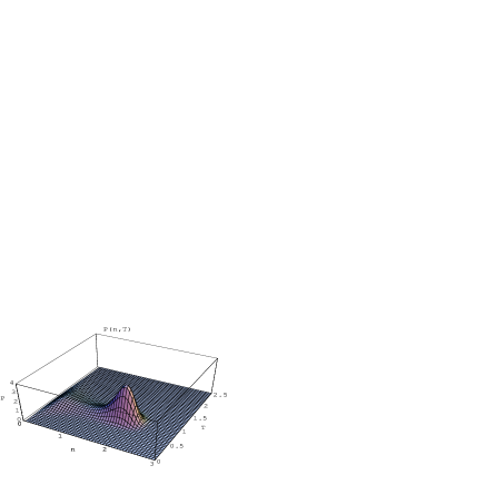
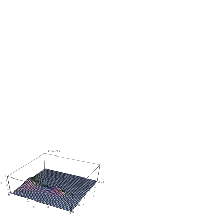
FIG. 5.: The distribution function $P(\tilde{n},\tilde{T})$ for an external temperature $1/\tilde{\beta}^{\rm ext}=0.85$. The external chemical potential is $\tilde{\mu}^{\rm ext}=-14.85$. The typical volume of the cells is $\tilde{V}=20$.

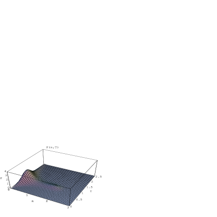
FIG. 6.: The distribution function $P(\tilde{n},\tilde{T})$ for an external temperature $1/\tilde{\beta}^{\rm ext}=0.85$. The external chemical potential is $\tilde{\mu}^{\rm ext}=-14.8971$. The typical volume of the cells is $\tilde{V}=20$. The two maxima have equal height.

FIG. 7.: The distribution function $P(\tilde{n},\tilde{T})$ for an external temperature $1/\tilde{\beta}^{\rm ext}=0.85$. The external chemical potential is $\tilde{\mu}^{\rm ext}=-14.95$. The typical volume of the cells is $\tilde{V}=20$.

In Figs. 7,7,7 we show the distribution of number density and temperature $P(\tilde{n},\tilde{T})$ for a value of the external temperature $1/\tilde{\beta}^{\rm ext}=0.85$ (below the unit critical temperature) and three different values of the external chemical potential $\tilde{\mu}^{\rm ext}=-14.85,-14.8971,-14.95$. We observe the presence of two humps at the same value of the temperature $\tilde{T}=0.85$ and different values of the density $\tilde{n}$. The existence of a bimodal structure in the distribution function $P(\tilde{n},\tilde{s})$ is a reflection of the gas-liquid transition, because a cell of size $\tilde{V}$ can have a non-vanishing probability of having two different values of the density. The external chemical potential $\tilde{\mu}^{\rm ext}$ controls the relative magnitude of the two maxima. For the particular value $\tilde{\mu}^{\rm ext}=-14.8971$, at this value of the external temperature, the two heights are equal. This value is called the chemical potential of coexistence and satisfies the equal area rule, see Fig. 4.

The size $\tilde{V}$ of the typical volume of a cell controls the sharpness of the distribution function. In Fig. 8, 9, 10 we show the distribution function $P(\tilde{n},\tilde{T}=0.85)$ for different values of $\tilde{V}$. The fluctuations become much smaller as $\tilde{V}$ becomes larger, consistent with the fact that in the thermodynamic limit fluctuations vanish. Another interesting property of the thermodynamic limit is that the relative height of the to peaks in the distribution function of the density increases as $\tilde{V}\rightarrow\infty$. Eventually only one of the two peaks survives. This is true, whenever the two peaks are not equal in height. When they are exactly equal both spikes coexist in the thermodynamic limit.

FIG. 8.: The distribution function $P(\tilde{n},\tilde{T})$ along the isotherm $\tilde{T}=0.85$ for two different values of $\tilde{V}=20$ (solid line) and $60$ (dotted line). Here, the external chemical potential is $\tilde{\mu}^{\rm ext}=-14.85$. Observe that the distribution becomes more peaked as the typical volume $\tilde{V}$ of the cells increases. The relative height increases and, eventually, in the thermodynamic limit $\tilde{V}\rightarrow\infty$ only one peak survives.

FIG. 9.: The distribution function $P(\tilde{n},\tilde{T})$ along the isotherm $\tilde{T}=0.8971$ for two different values of $\tilde{V}=20$ (solid line) and $60$ (dotted line). The chemical potential is that of coexistence, $\tilde{\mu}^{\rm ext}=-14.8971$. Because the heights are equal, as the typical volume $\tilde{V}$ of the cells increases, they remain equal at later times. In the thermodynamic limit two spikes localized at the gas and liquid densities remain.

FIG. 10.: The distribution function $P(\tilde{n},\tilde{T})$ at the critical point. The critical isotherm $\tilde{T}=1$ is plotted for $\tilde{\mu}^{\rm ext}=-17.36$ for two different values of $\tilde{V}=20$ (solid line) and $60$ (dotted line). Note the broad distribution of densities, which remain broad even in the thermodynamic limit.

IX Discussion

We have presented a Lagrangian finite Voronoi volume discretization of continuum hydrodynamics and have shown that the discrete equations have almost the GENERIC structure. The GENERIC structure can be restored by simply adding a small term into the reversible part of the dynamics. Therefore, the obtained equations conserve mass, momentum, and energy, and the entropy is an strictly increasing function of time in the absence of fluctuations. Thermal fluctuations are consistently included which lead to the strict increase of the entropy functional and to the correct Einstein distribution function. The size of the fluctuations is given by the typical size of the volumes of the particles, arguably scaling like the square root of this volume. The need of incorporating thermal fluctuations in a particular system will be determined by the external length scales that need to be resolved. For example, if sub-micron colloidal particles are considered, we need to resolve the size of the colloidal particle with fluid particles of size, say, an order of magnitude or two smaller than the diameter of the colloidal particle. For these small volumes, fluctuations are important and lead to the Brownian motion of the particle. A ping-pong ball, on the other hand requires fluid particles much larger, for which thermal fluctuations are negligible. Of course, one could use a very large number of small fluid particles to deal with the ping-pong ball, but in this case the (large) thermal fluctuations on each fluid particle average out among the (large) number of fluid particles.

The original formulations of Dissipative Particle Dynamics lack this effect of switching-off thermal fluctuations depending on the size of the fluid particles. This is due to the fact that early formulations did not include the volume and/or the mass of the particles as a relevant dynamical variable. In this paper, we have extended the range of variables and have shown that a thermodynamically consistent Dissipative Particle Dynamics model can be formulated. This model has the same reversible part as the finite Voronoi volume model. Hence, the usual conservative forces between dissipative particles are substituted by truly pressure forces. Therefore, prescribed thermodynamics can be given, without the need of “reverse inference” (find out which conservative force will produce the desired equation of state [9]). Even though the present DPD model has clear advantages over previous DPD models, it is yet inferior to the finite Voronoi volume model presented in this paper. Note that the finite volume is closely related to a discretization of Navier-Stokes equations, whereas the DPD model in this paper does not converge to the Navier-Stokes equations, even though it displays correct hydrodynamic behaviour. This means that in order to simulate a fluid of a given viscosity, one has to tune the viscosity parameter of the DPD model by previous simulation runs. With the finite volume model the true viscosity is given as input.

We have shown also that the Smoothed Particle Dynamics method has the GENERIC structure. However, we have pointed out several problems that favour the use of the finite volume method of the present paper. For example, in the Smoothed Particle Dynamics method we have noted that remnant forces appear even for the situation in which all particles are at rest with identical pressures. This effect can be made arbitrarily small by increasing the overlapping coefficient. But this has two drawbacks. The first one is of practical nature: when the overlapping coefficient is increased the number of interacting neighbours increases and, therefore, the computational time increases too. A second, more conceptual drawback is that in the large overlapping limit which, strictly speaking, is needed in order to “deduce” the SPH equations for Navier-Stokes, the volume (or density) of the particles becomes a constant and the equations start loosing its sense. The pressures, which depend essentially on the volumes, become a constant and the resulting equations cannot be claimed to be a faithful discretization of Navier-Stokes equations. Even though hydrodynamic behaviour is displayed (momentum is conserved locally) we expect that the thermodynamics and the transport properties of the simulated fluid differ from the actual desired values.

Concerning the GENERIC finite volume model of fluid particles presented in this paper, one of the most surprising realizations has been the fact that the mass of the fluid particles changes due to the reversible part of the dynamic. In Refs. [15], [23] this was overlooked. Of course, we could, in principle, formulate a model with ${\bf c}_{\mu\nu}=0$ in the final discrete equations (133). This would result in a great simplification of the equations without losing the desired GENERIC properties. This approximation would imply that the mass of the particles are constant. This spoils the equilibrium distribution function that would not be given by the Einstein distribution function (187) but rather by

$$\rho^{\rm eq}(x) = \frac{1}{\Omega}\prod_{\mu}^{M}\delta(M_{\mu}(x)-M_{\mu}^{0})\delta(E(x)-E_{0})\delta({\bf P}(x)-{\bf P}_{0}),$$ (238)

$$\times \exp\{k_{B}^{-1}S(x)\}$$ (239)

where $M_{\mu}^{0}$ is the initial value of the mass of particle $\mu$. In this case, not only total mass but also the individual masses are dynamical invariants of the discrete equations when ${\bf c}_{\mu\nu}=0$. We note that we could not follow the same arguments that lead to (231) and which describe the liquid-gas coexistence of a van der Waals fluid. This very same argument can be applied to the case of the SPH model discussed in section VII which renders the SPH model unsuitable to discuss gas-liquid coexistence. From a theoretical point of view, the possibility of simulating liquid-gas coexistence with a particle model represents a stringent condition on the thermodynamic consistency of the model proposed. Actually, we have learnt that the mass, and not the volume, of the fluid particles should be included as an independent dynamic variable if coexistence is to be described.

Finally, we would like to note that the model presente does not exibit the phenomena of surface tension. Surface tension can be easily included as an extra conservative contribution to the energy function [37].

X Appendix: Voronoi properties

In this appendix we explicitly compute the derivative of the volume of cell $\mu$ with respect to the position ${\bf R}_{\nu}$ of cell $\nu$, this is

$${\bf G}_{\mu\nu}=\frac{\partial{{\cal V}_{\mu}}}{{\partial{\bf R}_{\nu}}}=\frac{1}{\sigma^{2}}\int_{V_{T}}d{\bf R}\chi_{\mu}({\bf R})(\delta_{\mu\nu}-\chi_{\nu}({\bf R}))({\bf R}-{\bf R}_{\nu}).$$ (240)

Its worth considering the cases $\mu\neq\nu$ and $\mu=\nu$ explicitly.

$$\mbox{\boldmath$G$}_{\mu\nu} = -\frac{1}{\sigma^{2}}\int_{V_{T}}d{\bf R}\chi_{\mu}({\bf R})\chi_{\nu}({\bf R})({\bf R}-{\bf R}_{\nu}),\quad\quad\nu\neq\mu$$ (241)

$$\mbox{\boldmath$G$}_{\mu\mu} = \frac{1}{\sigma^{2}}\int_{V_{T}}d{\bf R}\chi_{\mu}({\bf R})(1-\chi_{\mu}({\bf R}))({\bf R}-{\bf R}_{\mu})$$ (242)

$$= \sum_{\nu\neq\mu}\frac{1}{\sigma^{2}}\int_{V_{T}}d{\bf R}\chi_{\mu}({\bf R})\chi_{\nu}({\bf R})({\bf R}-{\bf R}_{\mu})$$ (243)

$$= -\sum_{\nu\neq\mu}\mbox{\boldmath$G$}_{\nu\mu},$$ (244)

It is convenient to rewrite Eqn. (244) for $\nu\neq\mu$ as

$$\mbox{\boldmath$G$}_{\mu\nu} = -\frac{1}{\sigma^{2}}\int_{V_{T}}d{\bf R}\chi_{\mu}({\bf R})\chi_{\mu}({\bf R})\left({\bf R}-\frac{{\bf R}_{\mu}+{\bf R}_{\nu}}{2}\right)$$ (246)

$$-{\bf R}_{\mu\nu}\frac{1}{2\sigma^{2}}\int_{V_{T}}d{\bf R}\chi_{\mu}({\bf R})\chi_{\mu}({\bf R})$$

with ${\bf R}_{\mu\nu}={\bf R}_{\mu}-{\bf R}_{\nu}$. The first task is to compute the limit $\sigma\rightarrow 0$ for these two integrals. For this reason, it is instructive to work out the actual forms of $\chi_{\mu}({\bf R})$ and $\chi_{\mu}({\bf R})\chi_{\nu}({\bf R})$ for the case that only two particles are present in the system, as has been done by Flekkoy and Coveney [23]. Simple algebra leads to

$$\chi_{\mu}({\bf R}) = \frac{1}{1+\exp\{-{\bf R}_{\mu\nu}\!\cdot\!({\bf R}-({\bf R}_{\mu}+{\bf R}_{\nu})/2)/\sigma^{2}\}}$$ (247)

$$\chi_{\mu}({\bf R})\chi_{\nu}({\bf R}) = \frac{1}{4\cosh^{2}({\bf R}_{\mu\nu}\!\cdot\!({\bf R}-({\bf R}_{\mu}+{\bf R}_{\nu})/2)/2\sigma^{2}\})}$$ (248)

Note that $\chi_{\mu}({\bf R})\chi_{\nu}({\bf R})$ is different from zero only around the boundary of the Voronoi cells of particles $\mu,\nu$. In the limit of small $\sigma$ this is even more true. The integrals in (246) therefore can be performed not over the full volume ${V}_{T}$ but only over a region $\partial_{\mu\nu}$ “around” the boundary of the $\mu,\nu$ cells. In this region, we can further substitute the expression of $\chi_{\mu}({\bf r})\chi_{\nu}({\bf R})$, which depend on the positions of all the center cells, by Eqn. (LABEL:explicit), which depends only on the position of the centers of cells $\mu,\nu$. Actually, we can make a translation from ${\bf R}$ to ${\bf R}^{\prime}={\bf R}-({\bf R}_{\mu}+{\bf R}_{\nu})/2$ (we put the origin exactly at the boundary between cells). We can also make a rotation in such a way that the $x$ axis is along the line joining the cell centers. In this way, we can write

$$\frac{1}{\sigma^{2}}\int_{V_{T}}d{\bf R}\chi_{\mu}({\bf R})\chi_{\nu}({\bf R})$$ (250)

$$= \frac{1}{4\sigma^{2}}\int_{\partial_{\mu\nu}}d{\bf R}^{\prime}\frac{1}{\cosh^{2}({\bf R}^{\prime}\!\cdot\!{\bf R}_{\mu\nu}/2\sigma^{2})}$$ (251)

$$= \frac{1}{4\sigma^{2}}A_{\mu\nu}\int_{-\infty}^{\infty}dx\frac{1}{\cosh^{2}(xR_{\mu\nu}/2\sigma^{2})}$$ (252)

$$= \frac{A_{\mu\nu}}{R_{\mu\nu}}$$ (253)

Note that $\int_{0}^{\infty}\cosh^{-2}(x)dx=1$. Here, $A_{\mu\nu}$ is the actual area of the boundary between Voronoi cells of particles $\mu,\nu$.

In a similar way, one computes the first integral in Eqn. (246) with the result

$$\frac{1}{\sigma^{2}}\int_{V_{T}}d{\bf R}\chi_{\mu}({\bf R})\chi_{\mu}({\bf R})\left({\bf R}-\frac{{\bf R}_{\mu}+{\bf R}_{\nu}}{2}\right)=\frac{A_{\mu\nu}}{R_{\mu\nu}}{\bf c}_{\mu\nu}$$ (254)

where the vector ${\bf c}_{\mu\nu}$ is, by definition, the position of the center of mass of the face between Voronoi cells $\mu,\nu$ with respect to the point $({\bf R}_{\mu}+{\bf R}_{\nu})/2$. Collecting Eqns. (246),(254) and (253) one finally obtains

$$\mbox{\boldmath$G$}_{\mu\nu}=-A_{\mu\nu}\left(\frac{{\bf c}_{\mu\nu}}{R_{\mu\nu}}+\frac{{\bf e}_{\mu\nu}}{2}\right)$$ (255)

where

$${\bf e}_{\mu\nu} = \frac{{\bf R}_{\mu\nu}}{R_{\mu\nu}}$$ (256)

$${\bf R}_{\mu\nu} = {\bf R}_{\mu}-{\bf R}_{\nu}$$ (257)

$$R_{\mu\nu} = |{\bf R}_{\mu\nu}|$$ (258)

Note that $\sum_{\nu}{\bf G}_{\mu\nu}=0$ due to Eqn. (244). Also $\sum_{\mu}{\bf G}_{\mu\nu}=0$ because of Eqn. (240) and the fact that total volume is a constant, independent of positions.

XI Appendix: Dependent vs. independent variables in GENERIC

What happens if in the description of the state of a system one introduces, perhaps without knowing it, variables which are not independent of each other? We provide in this appendix the answer to this question.

Let us assume that the state of a system is described by a set of independent variables $x$. Assume, for the sake of simplicity, that the dynamics is purely reversible. The case $M\neq 0$ follows along a similar way as the one presented here for the reversible part.

Now assume that the basic building blocks of GENERIC have the following structure

$$E(x) = \overline{E}(x,y(x))$$ (259)

$$S(x) = \overline{S}(x,y(x))$$ (260)

$$L(x) = \overline{L}(x,y(x))$$ (261)

where $y(x)$ is a prescribed (vector) function of the sate $x$. From the chain rule one has

$$\nabla E(x)=\nabla_{x}\overline{E}(x,y(x))+J^{T}(x)\nabla_{y}\overline{E}(x,y(x))$$ (262)

and similarly for $S(x)$ and $L(x)$. Here, the matrix $J(x)$ is defined by $J(x)=\partial y/\partial x$.

The GENERIC reversible part of the dynamics is given by

$$\dot{x} = L(x)\nabla E(x)$$ (263)

$$= \overline{L}(x,y(x))\nabla_{x}\overline{E}(x,y(x))$$ (264)

$$+ \overline{L}(x,y(x))J^{T}(x)\nabla_{y}\overline{E}(x,y(x))$$ (265)

We can consider the time derivative of the functions $y(x(t))$ which, again through the chain rule, is given by

$$\dot{y}(x)=J(x)\dot{x}$$ (266)

By using now Eqn. (265) into (266) we can finally group both equation into the form

$$\left(\begin{array}[]{c}\dot{x}\\ \\ \dot{y}\\ \end{array}\right)=\left(\begin{array}[]{ccc}\overline{L}&&\overline{L}J^{T}\\ \\ J\overline{L}&&J\overline{L}J^{T}\\ \end{array}\right)\left(\begin{array}[]{c}\nabla_{x}\overline{E}\\ \\ \nabla_{y}\overline{E}\\ \end{array}\right)$$ (267)

or, by introducing the obvious notation $z=(x,y(x))$,

$$\dot{z}={\cal L}(z)\nabla_{z}E(z)$$ (268)

A very striking nicety is that the matrix ${\cal L}(z)$ has all the required properties for being a proper GENERIC reversible matrix. This is

$${\cal L}^{T}(z) = -{\cal L}(z)$$ (269)

$${\cal L}(z)\nabla_{z}S(z) = 0$$ (270)

$$\nabla_{z}[{\cal L}(z)\nabla_{z}E(z)] = 0$$ (271)

as can be easily checked from the properties of $L(x)$.

Now, let us assume that we start describing the state of a system by a vector $z=(x,y)$ and that the matrix $L(z)$ has the structure

$$\left(\begin{array}[]{ccc}\overline{L}(x,y)&&\overline{L}(x,y)J^{T}(x)\\ \\ J(x)\overline{L}(x,y)&&J(x)\overline{L}(x,y)J^{T}(x)\\ \end{array}\right)$$ (272)

with $J(x)=\partial h/\partial x$ for some set of functions $h(x)$. Then, we will have

$$\frac{d}{dt}y=\frac{\partial h}{\partial x}(x)\dot{x}=\frac{d}{dt}h(x)$$ (273)

and, therefore, $y=h(x)$. Therefore, if in a given model the matrix $L(z)$ happens to have the structure given in (272), then, necessarily, the variables $y$ are dependent on the variables $x$.

In our formulation in Ref. [15] we have assumed that the volume evolves according to

$$\dot{\cal V}_{\mu}=\sum_{\nu}{\bf\Omega}_{\mu\nu}\dot{\bf R}_{\nu}$$ (274)

which for most reasonable forms of ${\bf\Omega}_{\mu\nu}$ has the form of Eqn. (273). Therefore, the dynamical equation for the volume is nothing else than application of the chain rule and the volume cannot be considered as a truly independent variable of positions.

XII Appendix: Molecular ensemble

In this appendix we want to compute explicitly the following integral

$$\Phi({\bf P}_{0},E_{0},M) = \int d^{DM}{\bf P}\,\,\delta\!\left(\sum_{\mu}^{M}\frac{{\bf P}_{\mu}^{2}}{2M_{\mu}}-E_{0}\right)$$ (275)

$$\times \delta^{D}\!\left(\sum_{\mu}^{M}{\bf P}_{\mu}-{\bf P}_{0}\right)$$ (276)

$$= \prod_{\mu}^{M}(2M_{\mu})^{D/2}\int d^{DM}{\bf P}\,\,\delta\!\left(\sum_{\mu}^{M}{\bf P}_{\mu}^{2}-E_{0}\right)$$ (277)

$$\times \delta^{D}\!\left(\sum_{\mu}^{M}(2M_{\mu})^{1/2}{\bf P}_{\mu}-{\bf P}_{0}\right)$$ (278)

which appears repeatedly when computing molecular averages. The equation $\sum_{\mu}^{M}(2M_{\mu})^{1/2}{\bf P}_{\mu}={\bf P}_{0}$ are actually D equations (one for each component of the momentum) which define D planes in $R^{DM}$. The integral in (278) is actually over a submanifold which is the intersection of the D planes with the surface of a $DM$ dimensional sphere of radius $E_{0}^{1/2}$. This intersection will be also a sphere, which will be now of smaller radius and also of smaller dimension, $D(M-1)$.

In order to compute (278), we change to the following notation

$${\cal P} = (p_{1}^{x},\ldots,p_{M}^{x},p_{1}^{y},\ldots,p_{M}^{y},p_{1}^{z},\ldots,p_{M}^{z})$$ (279)

$$\mbox{\boldmath${\cal C}$}_{x} = ((2M_{1})^{1/2},\ldots,(2M_{M})^{1/2},0,\ldots,0,0,\ldots,0)$$ (280)

$$\mbox{\boldmath${\cal C}$}_{y} = (0,\ldots,0,(2M_{1})^{1/2},\ldots,(2M_{M})^{1/2},0,\ldots,0)$$ (281)

$$\mbox{\boldmath${\cal C}$}_{z} = (0,\ldots,0,0,\ldots,0,(2M_{1})^{1/2},\ldots,(2M_{M})^{1/2})$$ (282)

Note that these vectors satisfy $\mbox{\boldmath${\cal C}$}_{x}\!\cdot\!\mbox{\boldmath${\cal C}$}_{y}=0$ $\mbox{\boldmath${\cal C}$}_{y}\!\cdot\!\mbox{\boldmath${\cal C}$}_{z}=0$ $\mbox{\boldmath${\cal C}$}_{z}\!\cdot\!\mbox{\boldmath${\cal C}$}_{x}=0$. With these vectors so defined, Eqn. (278) becomes

$$\Phi({\bf P}_{0},E_{0},M) = \int d^{DM}\mbox{\boldmath${\cal P}$}\delta\!\left(\mbox{\boldmath${\cal P}$}^{2}-E\right)\,\,\delta\!\left(\mbox{\boldmath${\cal C}$}_{x}\!\cdot\!\mbox{\boldmath${\cal P}$}-P_{0}^{x}\right)$$ (283)

$$\times \,\,\delta\!\left(\mbox{\boldmath${\cal C}$}_{y}\!\cdot\!\mbox{\boldmath${\cal P}$}-P_{0}^{y}\right)\,\,\delta\!\left(\mbox{\boldmath${\cal C}$}_{z}\!\cdot\!\mbox{\boldmath${\cal P}$}-P_{0}^{z}\right)$$ (284)

$$\times \prod_{\mu}^{M}(2M_{\mu})^{D/2}$$ (285)

Now we consider the following change of variables

$$\mbox{\boldmath${\cal P}$}^{\prime}=\mbox{\boldmath${\cal P}$}-\left(\frac{\mbox{\boldmath${\cal C}$}_{x}}{|\mbox{\boldmath${\cal C}$}_{x}|^{2}}P_{0}^{x}+\frac{\mbox{\boldmath${\cal C}$}_{y}}{|\mbox{\boldmath${\cal C}$}_{y}|^{2}}P_{0}^{y}+\frac{\mbox{\boldmath${\cal C}$}_{z}}{|\mbox{\boldmath${\cal C}$}_{z}|^{2}}P_{0}^{z}\right)$$ (286)

which is simply a translation and has unit Jacobian. Simple algebra leads to

$$\Phi({\bf P}_{0},E_{0},M) = \prod_{\mu}^{M}(2M_{\mu})^{D/2}\int d^{DM}\mbox{\boldmath${\cal P}$}^{\prime}\,\,\delta\!\left(\frac{{\mbox{\boldmath${\cal P}$'}^{2}}}{2m}-U_{0}\right)$$ (287)

$$\times \delta\!\left(\mbox{\boldmath${\cal C}$}_{x}\!\cdot\!\mbox{\boldmath${\cal P}$}^{\prime}\right)\,\,\delta\!\left(\mbox{\boldmath${\cal C}$}_{y}\!\cdot\!\mbox{\boldmath${\cal P}$}^{\prime}\right)\,\,\delta\!\left(\mbox{\boldmath${\cal C}$}_{z}\!\cdot\!\mbox{\boldmath${\cal P}$}^{\prime}\right)$$ (288)

where we have introduced the total internal energy

$$U_{0}=\left(E_{0}-\frac{{\bf P}_{0}^{2}}{2{\cal M}_{0}}\right)$$ (289)

where ${\cal M}_{0}=\sum_{\mu}M_{\mu}$ is the total mass.

We now consider a second change of variables $\mbox{\boldmath${\cal P}$}^{\prime\prime}={\bf\Lambda}\!\cdot\!\mbox{\boldmath${\cal P}$}^{\prime}$ through a rotation ${\bf\Lambda}$ such that

$${\bf\Lambda}\mbox{\boldmath${\cal C}$}_{x} = (2{\cal M}_{0})^{1/2}(1,\ldots,0,0,\ldots,0,0,\ldots,0)$$ (290)

$${\bf\Lambda}\mbox{\boldmath${\cal C}$}_{y} = (2{\cal M}_{0})^{1/2}(0,\ldots,0,1,\ldots,0,0,\ldots,0)$$ (291)

$${\bf\Lambda}\mbox{\boldmath${\cal C}$}_{z} = (2{\cal M}_{0})^{1/2}(0,\ldots,0,0,\ldots,0,1,\ldots,0)$$ (292)

It is always possible to find a matrix ${\bf\Lambda}$ that satisfies Eqns. (292). For example, consider a block diagonal matrix made of three identical blocks of size $M\times M$. Then assume that each block is the same orthogonal matrix which transforms the vector $((2M_{1})^{1/2},(2M_{2})^{1/2},\ldots,(2M_{M})^{1/2})$ into $(2{\cal M}_{0})^{1/2}(1,0,\ldots,0)$. After the rotation (which has unit Jacobian and leaves the modulus of a vector invariant) the integral (288) becomes

$$\Phi = \prod_{\mu}^{M}(2M_{\mu})^{D/2}\int d^{DM}\mbox{\boldmath${\cal P}$}^{\prime\prime}\delta\!\left(\mbox{\boldmath${\cal P}$}^{\prime\prime 2}-U_{0}\right)$$ (293)

$$\times \,\,\delta((2{\cal M}_{0})^{1/2}p_{1}^{\prime\prime x})\,\,\delta((2{\cal M}_{0})^{1/2}p_{1}^{\prime\prime y})\,\,\delta((2{\cal M}_{0})^{1/2}p_{1}^{\prime\prime z})$$ (294)

$$= \prod_{\mu}^{M}(2M_{\mu})^{D/2}\int d^{D(M-1)}\mbox{\boldmath${\cal P}$}^{\prime\prime}\delta\!\left(\mbox{\boldmath${\cal P}$}^{\prime\prime 2}-U_{0}\right).$$ (295)

We compute now the integral over the sphere in Eqn. (295) by using that the integral of an arbitrary function $F({\bf x})=f(|{\bf x}|)$ that depends on ${\bf x}$ only through its modulus $|{\bf x}|$ can be computed by changing to polar coordinates

$$\int F({\bf x})d^{M}{\bf x}=\omega_{M}\int_{0}^{\infty}f(r)r^{M-1}dr.$$ (296)

The numerical factor $\omega_{M}$, which comes from the integration of the angles, can be computed by considering the special case when $f(r)$ is a Gaussian. The result is

$$\omega_{M}=2\frac{\pi^{M/2}}{\Gamma(M/2)}$$ (297)

By using Eqn. (296), Eqn. (295) becomes

$$\Phi({\bf P}_{0},E_{0},M) = \prod_{\mu}^{M}(2M_{\mu})^{D/2}\omega_{D(M-1)}$$ (298)

$$\times \int dp\,\,p^{D(M-1)-1}\,\,\delta\!\left(p^{2}-U\right)$$ (299)

We need now the property

$$\delta(f(x))=\sum_{\mu}\frac{\delta(x-x_{\mu})}{|f^{\prime}(x_{\mu})|}$$ (300)

where $x_{\mu}$ are the zeros of $f(x_{\mu})=0$. For the case of Eqn. (299) we have $f(x)=x^{2}-U$, $x_{\mu}=\pm(U)^{1/2}$ and $f^{\prime}(x)=2x$. Therefore,

$$\Phi({\bf P}_{0},E_{0},M)=\frac{1}{2}\omega_{D(M-1)}U_{0}^{\frac{D(M-1)-2}{2}}\prod_{\mu}^{M}(2M_{\mu})^{D/2}$$ (301)

XIII Appendix: van der Waals fluid

The free energy $F$ of a system has as natural variables the number of particles $N$, the temperature $T$ and the volume $V$, this is $F=F(N,T,V)$. Its derivatives are given by the pressure, the entropy and the chemical potential

$$-P = \left.\frac{\partial F}{\partial V}\right|_{T,N}$$ (302)

$$-S = \left.\frac{\partial F}{\partial T}\right|_{V,N}$$ (303)

$$\mu = \left.\frac{\partial F}{\partial N}\right|_{T,V}$$ (304)

Because the free energy is a first order function of the extensive variables $N,V$, we have

$$F(N,T,V)=Vf(n,T)$$ (305)

where $n$ is the number density and $f(n,T)$ is the free energy density. The property (305) implies in Eqns. (304)

$$-P(n,T) = f(n,T)-\mu n$$ (306)

$$s = -\frac{\partial f}{\partial T}(n,T)$$ (307)

$$\mu = \frac{\partial f}{\partial n}(n,T)$$ (308)

where $s=S/V$ is the entropy density.

For a van der Waals gas, the free energy density is given by

$$f(n,T)=-k_{B}Tn\left(1+\ln\left(\frac{1-nb}{n\Lambda^{D}(T)}\right)\right)-an^{2}$$ (309)

where the thermal wavelength is defined by

$$\Lambda(T)=\frac{h}{(2\pi m_{0}k_{B}T)^{1/2}}$$ (310)

Here, $h$ is Planck’s constant, $m_{0}$ is the mass of a molecule, and $k_{B}$ is Boltzmann constant. The constants $a,b$ are the attraction parameter and the excluded volume, respectively.

With Eqns. (308) plus the well-known relationship $f=\epsilon-Ts$ where $\epsilon$ is the internal energy density, we easily arrive at the following relations

$$\epsilon(n,s) = \frac{D}{2}k_{B}T(n,s)n-an^{2}$$ (311)

$$k_{B}T(n,s) = \left(\frac{h^{2}}{2\pi m_{0}}\right)\left(\frac{n}{1-nb}\right)^{2/D}\exp\left\{\frac{2s}{Dk_{B}n}-\frac{D+2}{D}\right\}$$ (312)

$$P(n,s) = \frac{k_{B}Tn}{1-nb}-an^{2}$$ (313)

$$\mu(n,s) = k_{B}T\left(\frac{nb}{1-nb}+\ln\left(\frac{nb}{1-nb}\right)\right)$$ (314)

$$- k_{B}T\ln\left(\frac{b}{\Lambda^{D}(T)}\right)-2an$$ (315)

which give the fundamental equation $\epsilon(n,s)$ and the three equations of state in terms of the variables $n,s$.

As it is customary for the van der Waals fluid, we introduce reduced variables

$$\tilde{T} = \frac{27b}{8a}k_{B}T,$$ (316)

$$\tilde{P} = \frac{27b^{2}}{a}P.$$ (317)

$$\tilde{\mu} = \frac{27b}{8a}\mu.$$ (318)

$$\tilde{n} = 3bn,$$ (319)

$$\tilde{s} = \frac{3bs}{k_{B}}$$ (320)

$$\tilde{\epsilon} = \frac{27b}{8a}3b\epsilon$$ (321)

In reduced units we have that the fundamental equation becomes

$$\tilde{\epsilon}(\tilde{n},\tilde{s})=\frac{D}{2}\tilde{T}(\tilde{n},\tilde{s})\tilde{n}-\frac{9}{8}\tilde{n}^{2}$$ (322)

and the three equations of state are

$$\tilde{T}(\tilde{n},\tilde{s}) = c\exp\frac{2}{D}\left\{\frac{\tilde{s}}{\tilde{n}}-\frac{D+2}{2}+\ln\left(\frac{\tilde{n}}{3-\tilde{n}}\right)\right\}$$ (323)

$$\tilde{P}(\tilde{n},\tilde{s}) = 8\frac{\tilde{T}\tilde{n}}{3-\tilde{n}}-3\tilde{n}^{2}$$ (324)

$$\tilde{\mu}(\tilde{n},\tilde{T}) = \tilde{T}\left(\ln\left(\frac{\tilde{n}}{3-\tilde{n}}\right)+\frac{\tilde{n}}{3-\tilde{n}}\right)-\frac{9}{4}\tilde{n}-\tilde{T}\ln\left(\frac{\tilde{T}}{c}\right)^{D/2}$$ (325)

In this equation, we have introduced the the constant $c$ which depends on microscopic parameters through

$$c=\frac{27b^{(D-2)/D}h^{2}}{16\pi m_{0}a}=4.836\times 10^{-5}$$ (326)

where we have used the values corresponding to water in $D=3$ dimensions, $a=1.5262\times 10^{-48}m^{5}kg/s^{2}$, $b=5.0622\times 10^{-29}m^{3}$, $m_{0}=2.991\times 10^{-26}kg$, $h=1.054\times 10^{-34}Js$ [38]. This constant appears in the the dimensionless quantity

$$\frac{b}{\Lambda^{D}(T)}=\left(\frac{\tilde{T}}{c}\right)^{D/2}$$ (327)

Note that in reduced units we still have the relationships

$$\frac{\partial\tilde{\epsilon}(\tilde{n},\tilde{s})}{\partial\tilde{n}} = \tilde{\mu}(\tilde{n},\tilde{s})$$ (328)

$$\frac{\partial\tilde{\epsilon}(\tilde{n},\tilde{s})}{\partial\tilde{s}} = \tilde{T}(\tilde{n},\tilde{s})$$ (329)

Let us focus now on the distribution function (233) which in reduced units becomes

$$P(\tilde{n},\tilde{s})=\frac{1}{Z}\exp\{\tilde{V}\left\{\tilde{s}-\tilde{\beta}^{\rm ext}(\tilde{\epsilon}(\tilde{n},\tilde{s})-\tilde{\mu}^{\rm ext}\tilde{n}\right\}$$ (330)

where $\tilde{V}=\overline{V}/3b$, $\tilde{\beta}^{\rm ext}=8a\beta/27b$, is the reduced inverse external temperature and $\tilde{\mu}^{\rm ext}=\overline{\lambda}m_{0}27b/8a$ is the reduced external chemical potential.

Due to the particular functional form of the fundamental equation for the van der Waals gas, it is more convenient to study the distribution function of $\tilde{n},\tilde{T}$ instead of $\tilde{n},\tilde{s}$. The Jacobian of the transformation is $\frac{D\tilde{n}}{2\tilde{T}}$ and, therefore, the new distribution function is

$$P(\tilde{n},\tilde{T})=\frac{\tilde{n}}{Z\tilde{T}}\exp\tilde{V}\{\tilde{s}(\tilde{n},\tilde{s})-\tilde{\beta}^{\rm ext}(\tilde{\epsilon}(\tilde{n},\tilde{s})-\tilde{\mu}^{\rm ext}\tilde{n})\}$$ (331)

REFERENCES

• [1] P.J. Hoogerbrugge and J.M.V.A. Koelman, Europhys. Lett. 19, 155 (1992)
• [2] P. Español and P. Warren, Europhys. Lett. 30, 191 (1995). P. Español, Phys. Rev. E, 52, 1734 (1995).
• [3] P. Español, Phys. Rev. E, 57, 2930 (1998).
• [4] C. Marsh, G. Backx, and M.H. Ernst, Europhys. Lett. 38, 411 (1997). C. Marsh, G. Backx, and M.H. Ernst, Phys. Rev. E 56, 1976 (1997).
• [5] J. Bonet Avalós and A.D. Mackie, Europhys. Lett. 40, 141 (1997). P. Español, Europhysics Letters 40, 631 (1997). M. Ripoll, P. Español, and M.H. Ernst, International Journal of Modern Physics C, 9, 1329 (1998).
• [6] J.M.V.A. Koelman and P.J. Hoogerbrugge, Europhys. Lett. 21, 369 (1993).
• [7] E.S. Boek, P.V. Coveney, H.N.W. Lekkerkerker, and P. van der Schoot, Phys. Rev. E 55, 3124 (1997).
• [8] A.G. Schlijper, P.J. Hoogerbrugge, and C.W. Manke, J. Rheol. 39, 567 (1995).
• [9] R.D. Groot and P.B. Warren, J. Chem. Phys. 107, 4423 (1997). R.D. Groot and T.J. Madden, J. Chem. Phys. 108, 8713 (1998). R.D. Groot, T.J. Madden, and D.J. Tildesley, J. Chem. Phys. 110, 9739, (1999).
• [10] P.V. Coveney and K. Novik, Phys. Rev. E 54, 5134 (1996). S.I. Jury, P. Bladon, S. Krishna, and M.E. Cates, Phys. Rev. 59 R2535 (1999). K. Novik and P.V. Coveney, Phys. Rev. E 61, 435 (2000).
• [11] W. Dzwinel and D.A. Yuen, Molecular Simulations, 22, 369 (1999).
• [12] L.B. Lucy, Astron. J. 82, 1013 (1977). J.J. Monaghan, Annu. Rev. Astron. Astrophys. 30, 543 (1992).
• [13] H. Takeda, S.M. Miyama, and M. Sekiya, Prog. Theor. Phys. 92, 939 (1994). H.A. Posch, W.G. Hoover, and O. Kum, Phys. Rev. E 52, 1711 (1995).
• [14] O. Kum, W.G. Hoover, and H.A. Posch, Phys. Rev. E 52, 4899 (1995).
• [15] P. Español, M. Serrano, and H.C. Öttinger, Phys. Rev. Lett. 83, 4542 (1999).
• [16] Eulerian implementations of fluctuating hydrodynamics have been considered by A.L. Garcia, M.M. Mansour, G.C. Lie, and E. Clementi, J. Stat. Phys. 47, 209 (1987) and H.-P. Breuer and F. Petruccione, Physica A 192, 569 (1993).
• [17] P. Mazur and D. Bedeaux, Physica 76, 235 (1974).
• [18] J. Güémez, S. Velasco, and A.C. Hernández, Physica A 152, 226, (1988), Physica A 152, 243, (1988), Physica A 153, 299, (1988). M. Rovere, D.W. Hermann, and K. Binder, Europhys. Lett. 6 585 (1988).
• [19] M.R. Swift, W.R. Osborn, and J.M. Yeomans, Phys. Rev. Lett. 75, 830 (1995). M.R. Swift, E. Orlandini, W.R. Osborn, and J.M. Yeomans, Phys. Rev. E 54 , 5041 (1996).
• [20] Li-Shi Luo, Phys. Rev. Lett. 81, 1618 (1998). A.D. ANgelopoulos, V.N. Paunov, V.N. Burganos, and A.C. Payatakes, Phys. Rev. E 57, 3237 (1998).
• [21] G.A. Bird, Molecular Gas Dynamics and the Direct Simulation of Gas flows, (Clarendon, Oxford 1994).
• [22] F. Alexander, A. Garcia and B. Alder, Physica A 240 196 (1997). N. Hadjiconstantinou, A. Garcia, and B. Alder, preprint “The Surface Properties of a van der Waals Fluid”.
• [23] E.G. Flekkoy and P.V. Coveney, Phys. Rev. Lett. 83, 1775 (1999). E.G. Flekkoy, P.V. Coveney, and G. De Fabritiis, preprint
• [24] D. Hietel, K. Steiner and J. Strucktmeier, Mathematical Models and Methods in Applied Sicence, in press.
• [25] X.-F. Yuan and M. Doi, Colloid and Surfaces A: Physicochemical and Engineering Aspects 144, 305 (1998).
• [26] X.-F. Yuan, R.C. Ball, and S.F. Edwards, J. Non-Newtonian Fluid Mech. 46, 331 (1993). X.-F. Yuan, R.C. Ball, and S.F. Edwards, J. Non-Newtonian Fluid Mech. 54, 423 (1994). X.-F. Yuan, R.C. Ball, J. Chem. Phys. 101, 9016 (1994), X.-F. Yuan, S.F. Edwards, J. Non-Newtonian Fluid Mech. 60, 335 (1995).
• [27] R. Zwanzig, J. Chem. Phys. 33, 1338 (1960), H. Mori, Prog. theor. Phys. 33, 423 (1965).
• [28] M. Grmela and H.C. Öttinger, Phys. Rev. E 56, 6620 (1997). H.C. Öttinger and M. Grmela, Phys. Rev. E 56, 6633 (1997). H.C. Öttinger, Phys. Rev. E 57, 1416 (1998).
• [29] H.C. Öttinger, J. Non-Equilib. Thermodyn. 22, 386 (1997). H.C. Öttinger, Physica A 254, 433 (1998).
• [30] J. Español and F.J. de la Rubia, Physica A 187, 589 (1992).
• [31] C.W. Gardiner, Handbook of Stochastic Methods, (Springer Verlag, Berlin, 1983). H. C. Öttinger, Stochastic Processes in Polymeric Fluids, Springer-Verlag, 1996.
• [32] An introduction to Voronoi tessellations and related computational geometry concepts can be found in http://www.voronoi.com. A particularly useful Java applet can be found in http://wwwpi6.fernuni-hagen.de/Geometrie-Labor/ VoroGlide/index.html.en .
• [33] S.R. de Groot and P. Mazur, Non-equilibrium thermodynamics (North-Holland Publishing Company, Amsterdam, 1962).
• [34] L.D. Landau and E.M. Lifshitz, Fluid Mechanics (Pergamon Press, 1959).
• [35] P. Español, Physica A 248, 77 (1998).
• [36] H.B. Callen Thermodynamics (John Wiley & sons, New York 1960).
• [37] Entropy for complex fluids M. Serrano and P. Español, preprint.
• [38] Handbook of Chemistry and Physics, 59th Edition, R.C. Wheast Ed. (CRC Press Inc, 1978).