Vortex lattice structures and pairing symmetry in Sr₂RuO₄

Abstract

Recent experimental results indicate that superconductivity in Sr₂RuO₄ is described by the $p$-wave $E_{u}$ representation of the $D_{4h}$ point group. Results on the vortex lattice structures for this representation are presented. The theoretical results are compared with experiment.

1 Introduction

The oxide Sr₂RuO₄ has a structure similar to high $T_{c}$ materials and was observed to be superconducting by Maeno et al. in 1994 [1]. It has been established that this superconductor is not a conventional $s$-wave superconductor: NQR measurements show no indication of a Hebel-Slichter peak in $1/T_{1}T$ [2], and $T_{c}$ is strongly suppressed below the maximum value of 1.5 K by non-magnetic impurities [3]. More recent experiments indicate an odd parity gap function of the form ${\bf d}({\bf k})=\hat{z}(\eta_{x}k_{x}+\eta_{y}k_{y})$. The Knight shift measurements of Ishida et al. [4] reveal that the spin susceptibility is unchanged upon entering the superconducting state; this is consistent with $p$-wave superconductivity (as predicted by Rice and Sigrist [5]). Furthermore, these measurements were conducted with the applied field in the basal plane. Since the orientation of the gap function (that is ${\bf d}$) is orthogonal to the spin projection of the Cooper pair [6], these measurements are consistent with the gap function aligned along the $\hat{z}$ direction. The $\mu$SR experiments of Luke et. al. have revealed spontaneous fields in the Meissner state [7]. This indicates that the superconducting order parameter must have more than one component [6, 7]. Naively, the observation of spontaneous fields leads to the conclusion that the superconducting gap function breaks time reversal symmetry (${\cal T}$) and therefore must have the form ${\bf d}({\bf k})=\hat{z}(k_{x}\pm ik_{y})$. However, the muons probe inhomogeneities in the superconducting state since any bulk magnetic fields are screened in the Meissner state. Consequently, ${\cal T}$ need only be broken in the vicinity of the inhomogeneities. For example, it has been pointed out in Ref. [6] that a gap function given by $\vec{\eta}=(1,\pm 1)$ can give rise to domain walls that break time reversal symmetry. In principle this can also lead to a $\mu$SR signal as seen by Luke et al.. Consequently, these two experiments lead to the gap function ${\bf d}({\bf k})=\hat{z}(\eta_{x}k_{x}+\eta_{y}k_{y})$, with the specific form of the order parameter $\eta_{x}$ and $\eta_{y}$ undetermined. In this talk, the vortex lattice structures arising in the phenomenological theory of this $E_{u}$ representation are examined. First, the theory is examined for an applied magnetic field in the basal plane along one of the two-fold symmetry axes. It is shown that multiple vortex lattice phases are generic to this representation. Then the weak-coupling limit of the theory is examined for the applied magnetic field along the $c$-axis. It is shown that a square vortex lattice results for parameters relevant to Sr₂RuO₄; consistent with the experimental observation of a square vortex lattice [8]. The theory of the square vortex lattice is compared with the observed results and good agreement is found.

2 Free Energy

The dimensionless free energy for the $E_{u}$ representation of $D_{4h}$ is given by [6]

$$f= -|\vec{\eta}|^{2}+|\vec{\eta}|^{4}/2+\beta_{2}(\eta_{x}\eta_{y}^{*}-\eta_{y}\eta_{x}^{*})^{2}/2$$

$$+\beta_{3}|\eta_{x}|^{2}|\eta_{y}|^{2}+|\tilde{D}_{x}\eta_{x}|^{2}+|\tilde{D}_{y}\eta_{y}|^{2}$$

$$+\kappa_{2}(|\tilde{D}_{y}\eta_{x}|^{2}+|\tilde{D}_{x}\eta_{y}|^{2})$$

$$+\kappa_{5}(|\tilde{D}_{z}\eta_{x}|^{2}+|\tilde{D}_{z}\eta_{y}|^{2})$$

$$+\kappa_{3}[(\tilde{D}_{x}\eta_{x})(\tilde{D}_{y}\eta_{y})^{*}+h.c.]$$

$$+\kappa_{4}[(\tilde{D}_{y}\eta_{x})(\tilde{D}_{x}\eta_{y})^{*}+h.c.]+h^{2}/(8\pi).$$

where $\tilde{D}_{j}=\nabla_{j}-\frac{2ie}{\hbar c}A_{j}$, ${\bf h}=\nabla\times{\bf A}$, and ${\bf A}$ is the vector potential. The stable homogeneous solutions are easily determined. There are three phases: (a) $\vec{\eta}=(1,i)/\sqrt{2}$ ($\beta_{2}>0$ and $\beta_{2}>\beta_{3}/2$), (b) $\vec{\eta}=(1,0)$ ($\beta_{3}>0$ and $\beta_{2}<\beta_{3}/2$), and (c) $\vec{\eta}=(1,1)/\sqrt{2}$ ($\beta_{3}<0$ and $\beta_{2}<0$). Phase (a) is nodeless and phases (b) and (c) have line nodes. For some of the discussion in this paper the Ginzburg Landau coefficients are determined within a weak-coupling approximation in the clean limit. In this case, taking for the $E_{u}$ REP the gap function described by the pseudo-spin-pairing gap matrix: $\hat{\Delta}=i[\eta_{1}v_{x}/\sqrt{\langle v_{x}^{2}\rangle}+\eta_{2}v_{y}/\sqrt{\langle v_{x}^{2}\rangle}]\sigma_{z}\sigma_{y}$, where the brackets $\langle\rangle$ denote an average over the Fermi surface and $\sigma_{i}$ are the Pauli matrices, it is found that [9] $\beta_{2}=\kappa_{2}=\kappa_{3}=\kappa_{4}=(\nu+1)/(3-\nu)$ and $\beta_{3}=4\nu/(3-\nu)$ where

$$\nu=\frac{\langle v_{x}^{4}\rangle-3\langle v_{x}^{2}v_{y}^{2}\rangle}{\langle v_{x}^{4}\rangle+\langle v_{x}^{2}v_{y}^{2}\rangle}.$$ (2)

Note that $|\nu|\leq 1$ and $\nu=0$ for a spherical or a cylindrical Fermi surface. Also note that $\vec{\eta}\propto(1,i)$ is the stable homogeneous state for all $\nu$.

3 Magnetic field in the basal plane

For the $E_{u}$ model, symmetry arguments imply that the vortex lattice phase diagram contains at least two vortex lattice phases for magnetic fields applied along at least two of the four two-fold symmetry axes [9]. To demonstrate this, consider the magnetic field along the $\hat{x}$ direction ($\hat{x}$ is chosen to be along the crystal ${\bf a}$ axis) and a homogeneous zero-field state $\vec{\eta}\propto(1,i)$. The presence of a magnetic field along the $\hat{x}$ direction breaks the degeneracy of the $(\eta_{x},\eta_{y})$ components, so that only one of these two components will order at the upper critical field [e.g. $\vec{\eta}\propto(0,1)$]. It has been shown for type II superconductors with a single component order parameter that the solution is independent of $x$ [10] so that $\sigma_{x}$ (a reflection about the $\hat{x}$ direction) is a symmetry operation of the $\vec{\eta}\propto(0,1)$ vortex phase. Now consider the zero-field phase $\vec{\eta}\propto(1,i)$; $\sigma_{x}$ transforms $(1,i)$ to $(-1,i)\neq e^{i\psi}(1,i)$ where $\psi$ is phase factor. This implies that $\sigma_{x}$ is not a symmetry operator of the zero-field phase. It follows that there must exist a second transition in the finite field phase at which $\eta_{x}$ becomes non-zero. Similar arguments hold for the field along any of the other three two-fold symmetry directions in the basal plane. Consequently a zero-field state $\vec{\eta}\propto(1,i)$ must exhibit two vortex lattice phases when the field is applied along any of the four two-fold symmetry axes. Similar arguments for $\vec{\eta}\propto(1,0)$ or $\vec{\eta}\propto(1,1)$. imply that there must exist at least two vortex lattice phases for only two of the four two-fold symmetry axes. For a zero-field state $\vec{\eta}=(1,0)$ fields along the $(1,1)$ or the $(1,-1)$ directions will result in two vortex lattice phases (for the $(1,0)$ and the $(0,1)$ directions multiple vortex lattice phases may exist, but are not required by symmetry). For a zero-field state $\vec{\eta}\propto(1,1)$, two vortex lattice phases will exist for fields along the $(1,0)$ or the $(0,1)$ directions.

An analysis of the free energy of Eq. 2 reveals additional information about the phase diagram [9, 11]. Assuming the large $\kappa$ limit (note $\kappa\approx 30$ for this field orientation in Sr₂RuO₄), the vector potential can be taken to be ${\bf A}=Hz(\sin\phi,-\cos\phi,0)$ ($\phi$ is the angle in the basal plane that the applied magnetic field makes with the $\hat{x}$ direction). The component of ${\bf D}$ along the field is set to zero. The upper critical field found by this method exhibits a four-fold anisotropy in the basal plane [9, 6]. For concreteness, the field is taken along the $\hat{x}$ direction ($\phi=0$). Introducing the raising and lowering operators $\Pi_{\pm}=q(\sqrt{\kappa_{2}/\kappa_{5}}D_{y}\pm iD_{z})/\sqrt{2}$ with $q^{2}=\sqrt{\kappa_{5}/\kappa_{2}}/H$, the gradient portion of the free energy can be written as

$$f_{grad}= \sqrt{\kappa_{5}\kappa_{2}}H\{\eta_{x}^{*}[1+2N]\eta_{x}+\eta_{y}^{*}[(\frac{1}{2}+\frac{1}{2\kappa_{2}})$$

$$(1+2N)+(\frac{1}{2\kappa_{2}}-\frac{1}{2})(\Pi_{+}^{2}+\Pi_{-}^{2})]\eta_{y}\}.$$

Assuming that $\kappa_{2}<1$ the first transition is given by the standard hexagonal Abrikosov vortex lattice solution for $\eta_{x}$. To find the second transition the lowest eigenstate of $(\frac{1}{2}+\frac{1}{2\kappa_{2}})(1+2N)+(\frac{1}{2\kappa_{2}}-\frac{1}{2})(e^{2i\theta}\Pi_{+}^{2}+e^{-2i\theta}\Pi_{-}^{2})$ must be found (where $\theta$ has been introduced so that the vortex lattice can be rotated with respect to the ionic lattice) and a vortex lattice solution for $\eta_{y}$ must be constructed from this. Note that the zeroes of the $\eta_{x}$ lattice and the zeroes of the $\eta_{y}$ lattice need not coincide [12]. This method yields for the ratio of the second transition ($H_{2}$) to the upper critical field ($H_{c2}$)

$$\frac{H_{2}}{H_{c_{2}}^{ab}}=\frac{\beta_{A}-\beta_{m}}{\beta_{A}\sqrt{1/\kappa_{2}}-\beta_{m}}$$ (3)

where $\beta_{A}=1.1596$, $\beta_{m}=(1-\beta_{2}+\beta_{3})S_{1}-|\beta_{2}S_{2}|$, $S_{1}=\overline{|\eta_{1}|^{2}|\eta_{2}|^{2}}/(\overline{|\eta_{1}|^{2}}\hphantom{a}\overline{|\eta_{2}|^{2}})$, $S_{2}=\overline{(\eta_{1}\eta_{2}^{*})^{2}}/(\overline{|\eta_{1}|^{2}}\hphantom{a}\overline{|\eta_{2}|^{2}})$, the over-bar denotes a spatial average, and $\beta_{m}$ must be minimized with respect to $\theta$ and the displacement between the zeros of the $\eta_{x}$ and the $\eta_{y}$ lattices. Diagrams of the predicted vortex structures are shown in Fig. 1 and the phase diagram for the weak-coupling limit is shown in Fig. 2. Two vortex lattice configurations are found to be stable as a function of $\nu$. For $-0.23<\nu<1$ (Phase 1), the displacement between the the zeroes of the $\eta_{x}$ and $\eta_{y}$ lattices is one half of a hexagonal lattice basis vector and $\theta$ varies with $\nu$ (and in general with field and temperature) so that the vortex lattice is not aligned with the ionic lattice. For $-1<\nu<-0.23$ (phase 2), the $\eta_{x}$ and $\eta_{y}$ lattices coincide and a vortex lattice basis vector lies along the $\hat{y}$ direction. Kita [11] has argued that for phase 1, at some field below $H_{2}$ there will be a first order transition from phase 1 to phase 2. For the field along $\hat{x}\pm\hat{y}$ the phase diagram is given by replacing $\nu$ with $-\nu$. Recent experiments of Mao et al. [13] show some support for the theory presented here.

Figure 1: Stable vortex lattice structures found for the field along $\hat{x}$. The open (closed) circles correspond to zeroes of the $\eta_{x}$ ($\eta_{y}$) lattice.

Figure 2: The ratio of the two transition fields and $\theta$ (the angle relating the orientation of the vortex lattice to the ionic lattice) as a function of $\nu$.

4 Magnetic field along the $c$-axis

The free energy in Eq. 2 in the weak coupling limit has been used to determine the vortex lattice structure for the field along the $c$-axis for fields near the upper critical field [14]. The main conclusion of this analysis is that vortex lattice is square for $|\nu|>0.0114$ and that the vortex lattice is oriented along the crystal lattice for $\nu<-0.0114$ and rotated 45 degrees from the crystal lattice for $\nu>0.0114$. The analysis near $H_{c1}$ has also been carried out with the result that the vortex lattice at $H_{c1}$ will be hexagonal and with increasing field the lattice will continuously distort until a square vortex lattice is formed [15]. A square vortex lattice has been observed by Small Angle Neutron scattering (SANS) and the orientation implies $\nu>0.0114$ [8]. One notable feature of the SANS measurements is the observation of Bragg peaks beyond the first Bragg peak. The analysis of Eq. 2 has been extended to fields below $H_{c2}$ and the lowest Bragg peaks of the field distribution have been calculated and compared to experiment. One comparison is shown in Fig. 3 (note that in the SANS measurements there is flux pinning which is not included in the calculations). The large size of the higher order Bragg peaks relative to that expected for a single complex order parameter component (Abrikosov) theory and the agreement between the theory and the experiment gives support to the $E_{u}$ theory. However, note that it is possible that an Abrikosov theory with sufficiently large non-local corrections may also account for the observed results.

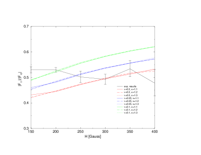
Figure 3: Comparison between the weak-coupling $E_{u}$ theory and experimental results for the ratio of the spatial Fourier components of the field corresponding to the $(1,0)$ and $(1,1)$ Bragg peaks of the square vortex lattice.

5 Acknowledgments

We acknowledge support from NSF DMR9527035 (DFA), the Swiss Nationalfonds, the U.K. E.P.S.R.C., and CREST of Japan Science and Technology Corporation. The neutron scattering was carried out at the Institut Laue-Langevin, Grenoble. We wish to thank T.M. Rice and M. Sigrist for informative discussions.

References

- [1] Y. Maeno et al., Nature 372, 532 (1994).
- [2] K. Ishida et al., Phys. Rev. B 56, 505 (1997).
- [3] A.P. Mackenzie et al., Phys. Rev. Lett. 80, 161 (1998).
- [4] K. Ishida et al., Nature (London) 96, 658 (1998).
- [5] T.M. Rice and M. Sigrist, J. Phys.: Condens. Matter 7, L643 (1995).
- [6] M. Sigrist and K. Ueda, Rev. Mod. Phys. 63, 239 (1991).
- [7] G.M. Luke et al., , Nature 394, 558 (1998).
- [8] T.M. Riseman et al., Nature 396, 242 (1998); and correction in press (2000).
- [9] D.F. Agterberg, Phys. Rev. Lett. 80, 5184 (1998).
- [10] I.A. Luk’yanchuk and M.E. Zhitomirsky, Supercond. Rev. 1, 207 (1995).
- [11] T. Kita, Phys. Rev. Lett. 83, 1846 (1999).
- [12] R. Joynt, Europhys. Lett. 16, 289 (1991); A. Garg and D.C. Chen, Phys. Rev. B 49, 479 (1994).
- [13] Z.Q. Mao et al., Phys. Rev. Lett. 84, 991 (2000).
- [14] D.F. Agterberg, Phys. Rev. B 58, 14 484 (1998).
- [15] R. Heeb and D.F. Agterberg, Phys. Rev. B 59, 7076 (1999).