Optimizing Traffic in Virtual and Real Space

Abstract

We show how optimization methods from economics known as portfolio strategies can be used for minimizing download times in the Internet and travel times in freeway traffic. While for Internet traffic, there is an optimal restart frequency for requesting data, freeway traffic can be optimized by a small percentage of vehicles coming from on-ramps. Interestingly, the portfolio strategies can decrease the average waiting or travel times, respectively, as well as their standard deviation (“risk”). In general, portfolio strategies are applicable to systems, in which the distribution of the quantity to be optimized is broad.

Virtual Traffic in the World Wide Web

Anyone who has browsed the World Wide Web has probably discovered the following strategy: whenever a web page takes too long to appear, it is useful to press the reload button. Very often, the web page then appears instantly. This motivates the implementation of a similar but automated strategy for the frequent “web crawls” that many Internet search engines depend on. In order to ensure up-to-date indexes, it is important to perform these crawls quickly. More generally, from an electronic commerce perspective, it is also very valuable to optimize the speed and the variance in the speed of transactions, automated or not, especially when the cost of performing those transactions is taken into account. Again, restart strategies may provide measurable benefits for the user.

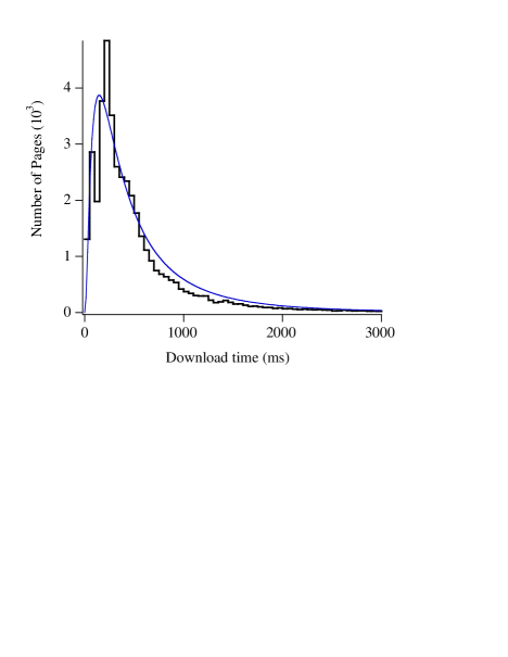
Figure 1: Latency distribution of the download times of the index.html file on the main page of over forty thousand web sites, with a fit to a log-normal distribution, see formula (5). The parameters are $\sigma=0.99$ and $\mu=5.97$.

The histogram in Figure 1 shows the variance associated with the download times for the text on the main page of over 40,000 web sites. Based on such observations, an economics-based strategy has recently been proposed for quantitatively managing the time of executing electronic transactions [1]. It exploits an analogy with the modern theory of financial portfolio management by associating cost with the time it takes to complete the transaction and taking into account the “risk” given by the standard deviation of that time. Before, such a strategy has already been successfully applied to the numerical solution of hard computational problems [2].

In modern portfolio theory, risk averse investors may prefer to hold assets from which they expect a lower return if they are compensated for the lower return with a lower level of risk exposure. Furthermore, it is a non-trivial result of portfolio theory that simple diversification can yield portfolios of assets which have higher expected return as well as lower risk. In the case of latencies (waiting times) on the Internet, thinking of different restart strategies is analogous to asset diversification: there is an efficient trade-off between the average time a request will take and the standard deviation of that time (“risk”).

Consider a situation in which data have been requested but not received (downloaded) for some time. This time can be very long in cases where the latency distribution has a long tail. One is then faced with the choice to either continue to wait for the data, to send out another request or, if the network protocols allow, to cancel the original request before sending out another. For simplicity, we consider the case in which it is possible to cancel the original request before sending out another one after waiting for a time period of duration $\tau$. If $p(t)$ denotes the probability distribution for the download time without restart, the probability $P(t)$ that a page has been successfully downloaded in time less than $t$ is given by

$$P(t)=\left\{\begin{array}[]{ll}p(t)&\mbox{ if }t\leq\tau\,,\\ &\\ \left[1-\int_{0}^{\tau}dt\;p(t)\right]P(t-\tau)&\mbox{ if }t>\tau\,.\end{array}\right.$$ (1)

As a consequence, the resulting average latency $\langle t\rangle$ and the risk $\sigma$ in downloading a page are given by

$$\langle t\rangle=\int\limits_{0}^{\infty}dt\;tP(t)$$ (2)

and

$$\sigma^{2}=\langle(t-\langle t\rangle)^{2}\rangle=\langle t^{2}\rangle-\langle t\rangle^{2}\,.$$ (3)

If we allow an infinite number of restarts, the recurrence relation (1) can be solved in terms of the partial moments $M_{n}(\tau)=\int_{0}^{\tau}dt\;t^{n}P(t)$:

$$\langle t\rangle = \frac{1}{M_{0}}\Big{[}M_{1}+\tau(1-M_{0})\Big{]}\,,$$

$$\langle t^{2}\rangle = \frac{1}{M_{0}}\left\{M_{2}+\tau(1-M_{0})\left[2\frac{M_{1}}{M_{0}}+\tau\left(\frac{2}{M_{0}}-1\right)\right]\right\}\,.$$ (4)

In the case of a log-normal distribution

$$p(t)=\frac{1}{\sqrt{2\pi}x\sigma}\exp\left(-\frac{{(\log x-\mu)^{2}}}{2\,\sigma^{2}}\right)\,,$$ (5)

$\langle t\rangle$ and $\langle t^{2}\rangle$ can be expressed in terms of the error function:

$$M_{n}(\tau)=\frac{1}{2}\exp\left(\frac{\sigma^{2}n^{2}}{2}+\mu n\right)\left[1+\mathrm{erf}\left(\frac{\log\tau-\mu}{\sigma\sqrt{2}}-\frac{\sigma n}{\sqrt{2}}\right)\right]\,.$$ (6)

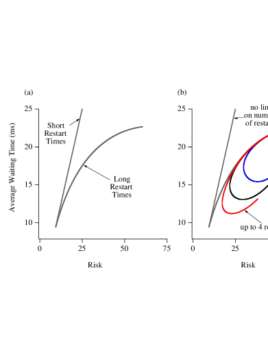
Figure 2: (a) Expected average latency versus risk calculated for a log-normal distribution with $\mu=2$ and $\sigma=1.5$. The curve is parametrized over a range of restart times $\tau$. (b) Family of curves obtained when we limit the maximum number of allowed restarts.

The resulting $\langle t\rangle$-versus-$\sigma$ curve is shown in Fig. 2(a). As can be seen, the curve has a cusp point that represents the restart time $\tau$ that is preferable to all others. No strategy exists in this case with a lower expected waiting time or with a lower variance. The location of the cusp can be translated into the optimum value of the restart time to be used to reload the page.

There are many variations to the restart strategy described above. In particular, in Fig. 2(b), we show the family of curves obtained from the same distribution used in Fig. 2(a), but with a restriction on the maximum number of restarts allowed in each transaction. Even a few restarts yield an improvement.

Clearly, in a network without any kind of usage-based pricing, sending many identical data requests, to begin with, would be the best strategy as long as we do not overwhelm the target computer. On the other hand, everyone can reason in exactly the same way, resulting in congestion levels that would render the network useless. This paradoxical situation, sometimes called a social dilemma, arises often in the consideration of ”public goods” such as natural resources and the provision of services which require voluntary cooperation [3]. This explains much of the current interest in determining the details of an appropriate pricing scheme for the Internet, since users do consume Internet bandwidth greedily when downloading large multimedia files for example, without consideration of the congestion caused by such activity.

Note that the histogram in Figure 1 represents the variance in the download time between different sites, whereas a successful restart strategy depends on a variance in the download times for the same document on the same site. For this reason, we cannot use the histogram in Figure 1 to predict the effectiveness of the restart strategy, but need to apply the similarly looking distribution of the respective Internet site. While a spread in the average download times of pages from different sites reduces the gains that can be made using a common restart strategy, it is possible to take advantage of geography and the time of day to fine tune and improve the strategy’s performance. As a last resort, it is possible to fine tune the restart strategy on a site per site basis.

As a final caution, we point out that with current client-server implementations, multiple restarts are detrimental and very inefficient since every duplicated request will enter the server’s queue and are processed separately until the server realizes that the client is not listening to the reply. This is an important issue for a practical implementation, and we neglect it here: our main assumption is that the restart strategy only affects the congestion by modifying the perceived latencies. This is only true if the restart strategy is implemented in an efficient and coordinated way on both the client and server side.

Real Traffic on Freeways with Ramps

The recent study of the properties of “synchronized” congested highway traffic [4] has generated a strong interest in the rich spectrum of phenomena occuring close to on-ramps [5, 6]. In this connection, a particularly relevant problem is that of choosing an optimal injection strategy of vehicles into the highway. While there exist a number of heuristic approaches to optimizing vehicle injection into freeways by on-ramp controls, the results are still not satisfactory. What is needed is a strategy that is flexible enough to adapt in real time to the transient flow characteristics of road traffic while leading to minimal travel times for all vehicles on the highway.

Our study presents a solution to this problem that explicitly exploits the naturally occuring fluctuations of traffic flow in order to enter the freeway at optimal times. This method leads to a more homogeneous traffic flow and a reduction of inefficient stop-and-go motions. In contrast to conventional methods, the basic performance criterion behind this technique is not the traffic volume, the optimization of which usually drives the system closer to the instability point of traffic flow and, hence, reduces the reliability of travel time predictions [7]. Instead, we will focus on the optimization of the travel time distribution itself, which is a global measure of the overall dynamics on the whole freeway stretch. It allows the evaluation of both the expected (average) travel time of vehicles and their variance, where a high value of the variance indicates a small reliability of the expected travel time when it comes to the prediction of individual arrival times.

Both the average and the variance of travel times are influenced by the inflow of vehicles entering the freeway over an on-ramp. From these two quantities one can again construct a relation between the average payoff (the negative mean value of travel times) and the risk (their standard deviation). The optimal strategy will then correpond to the point in the curve that yields the lowest risk at a high average payoff. In the following, we will show that the variance of travel times has a minimum for on-ramp flows that are different from zero, but only in the congested traffic regime (which shows that the effect is not trivial at all). This finding implies that traffic flow can be optimized by choosing the appropriate vehicle injection rate into the freeway. Hence, in order to reach well predictable and small average travel times at high flows in the overall system, it makes sense to temporarily hold back vehicles by a suitable on-ramp control based on a traffic-dependent stop light [8]. At intersections of freeways, this may require additional buffer lanes [9].

In order to obtain the travel time distribution of vehicles on a highway, we simulated traffic flow via a discretized and noisy version of the optimal velocity model by Bando et al. [10], which describes the empirical known features of traffic flows quite well [11]. Moreover, we extended the simulation to several lanes with lane-changing maneuvers and different vehicle types (fast cars and slow trucks) [12, 13]. For lane changes, we assumed symmetrical (“American”) rules, i.e. vehicles could equally overtake on the left-hand or on the right-hand lane. Lane changing maneuvers were performed, when an incentive criterion and a safety criterion were satisfied [14]. The incentive criterion was fulfilled, when a vehicle could go faster on the neighboring lane, while the safety criterion required that lane changing would not produce any accident (i.e., there had to be a sufficiently large gap on the neighboring lane) [12, 13].

In addition to a two-lane stretch of length $L=10$ km, we simulated an on-ramp section of length 1 km with a third lane that could not be used by vehicles from the main road. However, vehicles entered the beginning of the on-ramp lane at a specified injection rate. Injected vehicles tried to change from the on-ramp to the main road as fast as possible, i.e. they cared only about the safety criterion, but not about the incentive criterion. The end of the on-ramp was treated like a resting vehicle, so that any vehicle that approached it had to stop, but it changed to the destination lane as soon as it found a sufficiently large gap. If the on-ramp was completely occupied by vehicles waiting to enter the main road, the injected vehicles formed a queue and entered the on-ramp as soon as possible. After injected vehicles had completed the 10 kilometer long two-lane measurement stretch, they were automatically removed from the freeway [13].

Our simulations were carried out for a circular road. After the overall density was selected, vehicles were homogeneously distributed over the road at the beginning, with the same densities on both lanes of the main road. The experiments started with uniform distances among the vehicles and their associated optimal velocities. The vehicle type was determined randomly after specifying the percentages $r$ of cars ($\geq$ 90%) and $(1-r)$ of trucks ($\leq$ 10%). Notice that the effects discussed in the following should be more pronounced for increased $r(1-r)$, since lane-changing rates seem to be larger and traffic flow more unstable, then.

Figure 3: Examples of travel time distributions for mixed traffic composed of a majority of cars and a minority of trucks. (a) A narrow distribution results for stable traffic flow. (a) For unstable traffic flow, the distribution is broad. (In the simulations underlying the above results, no vehicles were injected to the main road over the on-ramp.)

We determined the travel times of all vehicles by calculating the difference in the times at which they passed the beginning and the end of the 10 kilometer long two-lane section. For mixed traffic composed of a high percentage of cars and a small percentage of slower trucks, we found narrow travel time distributions at small vehicle densities, where traffic flow was stable, while for unstable traffic flow at medium densities, the travel time distributions were broad (see Fig. 3).

Figure 4: Average and standard deviation of the travel times of vehicles on the main road and from the ramp as a function of the injection rate $Q_{\rm rmp}=1/(n{\rm\ s})$ with $n=2^{k}$ and $k\in\{2,3,\dots,10\}$ for various vehicle densities on the main road (measured without injection). With increasing injection rate, the average travel times are growing due to the higher resulting vehicle density on the freeway. However, at high enough vehicle densities, the standard deviation shows minima for medium interaction rates. Injected vehicles require longer travel times, since they cause a more crowded destination lane. (After [13].)

If we plot the average of travel times as a function of their standard deviation (Fig. 4), we obtain curves parametrized by the injection rate of vehicles into the road and find the following: 1. With growing injection rate

$$Q_{{\rm rmp}}=\frac{1}{n{\rm\ s}}\,,$$ (7)

the travel time increases monotonically. This is because of the increased density caused by injection of vehicles into the freeway. 2. The average travel time of injected vehicles is higher, but their standard deviation lower than for the vehicles circling on the main road. This is due to the fact that vehicle injection produces a higher density on the lane adjacent to the on-ramp, which leads to smaller velocities. The difference between the travel time distributions of injected vehicles and those on the main road decreases with the length $L$ of the simulated road, since lane-changes tend to equilibrate densities between lanes.

In addition, the standard deviation of the travel times has a minimum for finite injection rates, as entering vehicles tend to fill existing gaps and thus homogenize traffic flow. This minimum is optimal in the sense that there is no other value of the injection rate that can produce travel with smaller variance. In particular, gap-filling behavior mitigates inefficient stop-and-go traffic at medium densities. Above a density of 45 vehicles per kilometer and lane on the main road (measured without injection), the minimum of the travel times’ standard deviation occurs for $n\approx 60$. The reduction of the average travel time by smaller injection rates is less than the increase of their standard deviation. This result suggests that, in order to generate predictable and reliable arrival times, one should operate traffic at medium injection rates. For the case of 40 vehicles per kilometer and lane, the minimum of the standard deviation of travel times is located at $n\approx 30$, while for 35 vehicles per kilometer and lane, it is at $n\approx 15$. Below about 25 vehicles per kilometer and lane, vehicle injection does not reduce the standard deviation of travel times, since the travel time distribution is narrow anyway. At these densities, traffic flow is stable and homogeneous, so that no inefficient stop-and-go traffic exists and therefore no large gaps can be filled [12].

Figure 5: As Fig. 4, but as a function of the resulting effective density $\rho_{\rm eff}$ on the freeway rather than the density $\rho_{\rm main}$ on the main road without injection. We find shorter travel times at high injection rates because of the homogenization of traffic. The standard deviation of travel times is varying stronger than the average travel time, which indicates that medium injection rates are the optimal choice at high vehicle densities. At small vehicles densities, the standard deviation does not show a minimum, since traffic flow is homogeneous anyway. (After [13].)

The curves displayed in Fig. 4 correspond to a given density $\rho_{{\rm main}}$ on the main road without injection of vehicles. The effective density $\rho_{{\rm eff}}$ on the freeway resulting from the injection of vehicles can be approximated by

$$\rho_{{\rm eff}}=\rho_{{\rm main}}+\frac{N_{{\rm inj}}}{IL}\,,$$ (8)

where $I=2$ lanes, $L=10$ km. $N_{{\rm inj}}$ is the average number of injected vehicles present on the main road and can be written as

$$N_{{\rm inj}}=N_{{\rm tot}}\frac{{\cal T}_{{\rm inj}}}{{\cal T}_{{\rm tot}}-{\cal T}_{{\rm inj}}}\,,$$ (9)

where $N_{{\rm tot}}=1000$ is the total number of injected vehicles during the simulation runs, ${\cal T}_{{\rm inj}}$ is their average travel time, and ${\cal T}_{{\rm tot}}$ the time interval needed by all $N_{{\rm tot}}=1000$ vehicles to complete their trip. We point out that, in addition to these measurements, we used two other methods of density measurement which yielded similar results.

In contrast to Fig. 4, we also computed the dependence of the travel time characteristics on the resulting effective densities of vehicles. Fig. 5 shows the average of the travel times for vehicles in the main road as a function of their standard deviation. Once again, we observe a minimum of the standard deviation of travel times at high vehicle densities and medium injection rates. However, this time, an increase of the injection rate reduces the average travel times!

Figure 6: Average travel times of vehicles on the main road as a function of the resulting effective vehicle density on the freeway for various injection rates $Q_{\rm rmp}=1/(n{\rm\ s})$ ($n\in\{2,3,4,5,10\}$). Obviously, the travel times are reduced by vehicle injection, which comes from a reduction of inefficient stop-and-go traffic. In the limit of high injection rates, one observes a linear dependence of average travel times on effective density, which is in agreement with analytical results [13]. We mention that the travel times of injected vehicles did not depend on the injection rate. However, when we checked what happens if the vehicles on the main road try to change to the left lane along the on-ramp in order to give way to entering vehicles (as they do in many European countries), we found that both, injected vehicles and the vehicles on the main road, profited from this behavior. (After [13].)

Figure 6 investigates the surprising reduction of the average travel times in more detail. While the injected cars experienced travel times that agreed with the case of no injection, the vehicles on the main road clearly profited from vehicle injection, if the effective density was the same. This means that, for given $\rho_{\rm eff}$, one can actually increase the average velocity $V_{{\rm main}}=L/{\cal T}_{{\rm main}}$ of vehicles by injecting vehicles at a considerable rate without affecting their travel times. This result is due to the increased degree of homogeneity caused by entering vehicles that fill gaps on the main road, which mitigates the less efficient stop-and-go traffic.

We point out that the injection-based reduction of travel times on the main road at a given effective density $\rho_{\rm eff}$ is related with a higher proportion

$$P=1-\frac{\rho_{\rm main}}{\rho_{\rm eff}}$$ (10)

of injected vehicles, which implies a reduction in the number of vehicles circling on the main road. The relation between the injection rate and the percentage of injected vehicles is roughly linear (see Fig. 7).

Figure 7: Proportion of injected vehicles as a function of the injection rate $Q_{\rm rmp}$.

The dependencies of the average travel times and their standard deviation on the proportion of injected vehicles are depicted in Figure 8. We find that the decrease in the average travel times is minor, while a significant reduction of the variance of travel times can be achieved by less than 5% of injected vehicles.

Figure 8: (a) Average travel times and (b) their standard deviation as a function of the proportion of injected vehicles.

Summary and Conclusions

Portfolio strategies can be successfully applied to systems in which the distribution of the quantity to be optimized is broad. This is the case for the download times in the World Wide Web as well as the travel time distributions in congested traffic flow. In this article, we showed how to reduce the average waiting times as well as their standard deviation (“risk”) by suitable injection strategies. In the case of the World Wide Web, it is possible to enforce smaller average waiting times by restarting a data request when the data were not received after a certain time interval $\tau$. This deforms the waiting time distribution towards smaller values, which automatically reduces the variance as well. Since the long tail of the waiting time distribution comes from the intermittent (“bursty”) behavior of Internet traffic, restart strategies partially manage to “calm down” these “Internet storms” by withdrawing requests in busy periods and restarting them later on. Similarly, the injection of vehicles to a freeway over an on-ramp can homogenize inefficient stop-and-go traffic by filling large gaps. In other words: The strategy exploits the naturally occuring fluctuations of traffic flow in order to allow the entry of new vehicles to the freeway at optimal times. In this way, the variation of travel times can be considerably reduced, which is favourable for more reliable travel time predictions. Moreover, at a given effective density, the average travel time decreases with increasing injection rate, i.e., with an increasing percentage of injected vehicles on the main road.

Acknowledgments: D.H. wants to thank the German Research Foundation (DFG) for financial support (Heisenberg scholarship He 2789/1-1). S.M. thanks for financial support by the Hertz Foundation.

References

- [1] Lukose, R. M. and Huberman, B. A.: A methodology for managing risk in electronic transactions over the internet. Netnomics, in press (2000).
- [2] Huberman, B. A., Lukose, R. M., and Hogg, T.: An economics approach to hard computational problems. Science 275 (1997) 51.
- [3] Hardin, R.: Collective Action (Johns Hopkins University Press, 1982).
- [4] Kerner, B. S. and Rehborn, H.: Experimental properties of phase transitions in traffic flow. Phys. Rev. Lett. 79 (1997) 4030; Kerner, B. S. and Rehborn, H.: Experimental properties of complexity in traffic flow. Phys. Rev. E 53 (1996) R4275.
- [5] Lee, H. Y., Lee, H.-W., and Kim, D.: Origin of synchronized traffic flow on highways and its dynamic phase transition. Phys. Rev. Lett. 81 (1998) 1130.
- [6] Helbing, D. and Treiber, M.: Gas-kinetic-based traffic model explaining observed hysteretic phase transition. Phys. Rev. Lett. 81 (1998) 3042; Helbing, D. and Treiber, M.: Jams, waves, and clusters. Science 282 (1998) 2001; Helbing, D., Hennecke, A., and Treiber, M.: Phase diagram of traffic states in the presence of inhomogeneities. Phys. Rev. Lett. 82 (1999) 4360.
- [7] Nagel, K. and Rasmussen, S.: Traffic at the edge of chaos. In: Artificial Life IV, edited by R. A. Brooks and P. Maes (MIT Press, Cambridge, MA, 1994).
- [8] Helbing, D.: New simulation models for traffic optimization. In: Proceedings of the Workshop “Verkehrsplanung und -simulation”, edited by V. Claus, D. Helbing, and H. J. Herrmann (Informatik Verbund Stuttgart, University of Stuttgart, 1999).
- [9] Bovy, P. H. L. (ed.): Motorway Traffic Flow Analysis (Delft University Press, Delft, 1998).
- [10] Bando, M., Hasebe, K., Nakanishi, K., Nakayama, A., Shibata, A., and Sugiyama, Y.: Phenomenological study of dynamical model of traffic flow. Journal de Physique I (France) 5 (1995) 1389.
- [11] Helbing, D. and Schreckenberg, M.: Cellular automata simulating experimental properties of traffic flows. Phys. Rev. E 59 (1999) R2505.
- [12] Helbing, D. and Huberman, B. A.: Coherent moving states in highway traffic. Nature 396 (1998) 738.
- [13] Huberman, B. A. and Helbing, D.: Economics-based optimization of unstable flows. Europhysics Letters 47 (1999) 196.
- [14] Nagel, K., Wolf, D. E., Wagner, P., and Simon, P.: Two-lane traffic rules for cellular automata: A systematic approach. Phys. Rev. E 58 (1998) 1425.