Dynamics of aeolian sand ripples

Abstract

We analyze theoretically the dynamics of aeolian sand ripples. In order to put the study in the context we first review existing models. This paper is a continuation of two previous papers[3, 4], the first one is based on symmetries and the second on a hydrodynamical model. We show how the hydrodynamical model may be modified to recover the missing terms that are dictated by symmetries. The symmetry and conservation arguments are powerful in that the form of the equation is model-independent. We then present an extensive numerical and analytical analysis of the generic sand ripple equation. We find that at the initial stage the wavelength of the ripple is that corresponding to the linearly most dangerous mode. At later stages the profile undergoes a coarsening process leading to a significant increase of the wavelength. We find that including the next higher order nonlinear term in the equation, leads naturally to a saturation of the local slope. We analyze both analytically and numerically the coarsening stage, in terms of a dynamical exponent for the mean wavelength increase. We discuss some future lines of investigations.

PACS numbers: 83.70.Fn,81.05.Rm,47.20.-k

1 Introduction

Perhaps the most ancient and fascinating out-of-equilibrium example of spontaneous pattern formation known in nature is that exhibited by a sand bed subjected to wind. If wind is strong enough (but not too strong to prevent erosion), of the order of few m/s, sand grains enter into a perpetual motion causing ultimately the sand bed to become unstable to ripple formation, commonly referred to as aeolian sand ripples. The typical wavelength is of the order of few cm (in some deserts, in Libya, however, ripples continue to coarsen leading to wavelengths which are much larger – several m –, and are usually called ridges). Geologists, in particular, have been intrigued that such an apparently simple system as sand turns from an intially structureless state into a rather organized structure in a quite robust and reproducible fashion, despite the turbulent air flow that causes the ripple formation. Following the seminal work of Bagnold [1] many researchers have achieved a significant contribution to the understanding of ripple formation both experimentally and theoretically. This field of research has known more recently an upsurge of interest as a part of the puzzling behaviour of granular media. Despite the fact that sand is a very familiar material, the understanding of its static and dynamical properties still poses a formidable challenge to theoretical modelling. Unlike elastic, viscoelastic materials, and Newtonian fluids, there is yet no universal continuum theory (such that leading to the Lamé or Navier-Stokes equations) to describe in a effective manner the behaviour of granular media. A major difficulty, in our opinion, lies in the broad spectrum of length and time scales. Despite this situation, various tools have been used to describe in a more or less ad hoc way granular media. With regard to ripple formation, we may cite (i) molecular dynamics introducing empirical laws of collision, (ii) Monte Carlo simulations, trying to mimic what is our feeling about rules of collision and rearrangements, (iii) hydrodynamical theories inspired from Bagnold’s view. Concerning the birth of ripples the view of Bagnold is largely adopted and it will be reviewed shortly here.

An important preliminary question is in order. Indeed, even without evoking the possibility of writing basic sand equations, we may ask a fundamental question about locality-versus-nonlocality in the aeolian sand ripple formation. More precisely does dynamics of a given region (small in comparison to the ripple wavelength) depend on that of a distant region located at a distance which is significantly larger than the ripple wavelength? If so we can say that sand surface dynamics must be nonlocal. This question is still controversial, and it seems to us very important to settle it up from the very beginning. The argument in favour of nonlocality rests on the following fact: because the grains that make a high fly (the saltation grains – Fig. 1) possess a saltation length $l$ which is much larger than the ripple wavelength $\lambda$, then a rather distant region on the sand bed would get these saltating particles. As information is being passed from two quite distant points, we would a priori think of the importance of nonlocality. In reality, the moving grains in the ripple formation process can divided into two main categories: the saltating ones that have a high kinetic energy (and make long jumps) and the low energy splashed grains (dislodged by the impact of saltating grains – see Fig.1) which in turn travel in a hopping manner on a scale $a$ which is several (typically 6–10) times smaller that the ripple wavelength. If nonlocality is adopted we must answer these two experimental facts which clearly contradict it: (i) as noted by Bagnold the saltating grains population arrives on the sand bed almost at the same angle everywhere along the bed – as if a rain of particles were sent from a very long altitude at a fixed incident angle (which is of order of $10^{\circ}$); so when they impact on a region there is no way to distinguish between, say, two gains that originate from two different regions of the sand surface. (ii) Additionally, as a grain has been extracted from the bed, becoming thereby a saltating one, it is transported by a turbulent flow where at a such high Reynolds number the coherence length is so small that during the fly the grains loose, so to speak, the memory of where it comes from. Given these two facts it is hard to believe that saltating grains provides any effective interaction between the topography of two distant regions on the surface. Thus it seems difficult to be in favour of nonlocality, albeit saltating grains make, beyond any doubt, long jumps. Their high jumps simply imply that their energy is such that they can dislodge some grains (the reptating grains) and make them jump on a length scale $a$. If the saltating grains had a higher energy, then $a$ would be increased which in turn (as seen also experimentally [2]) would increase the ripple wavelength, keeping $\lambda/a$ to a typical value of order $6-10$. In other words, and as again noted by Bagnold[1], and reported by Anderson et al.[2], the saltating grains serve merely to bring energy into the system, the saltating population exchanges almost no grains with the reptating population. The ripple formation depends basically on the local topography of surface, and the information is propagated only by reptating grains. We believe that we can even conceive the following experiment: we use an air gun designed to throw beads and inclined with some angle with respect to an intially flat bead surface. Then we move the air gun over the bed in a erratic fashion, back and forth, and send beads on the bed. After a sufficiently large number of collisions the bead surface should develop a ripple structure. By this way we completely eliminate any notion of saltation; the air gun is simply injecting energy into the system.

The initiation of sand ripples as imagined by Bagnold is appealing (see later). However, a question of major importance has remained open until recently: once the instability takes place, what is the subsequent evolution of the instability? Would the instability lead to an ordered or disordered structure? Would the wavelength be that corresponding to the linearly fastest growing mode? The initiation of the instability is based on a linear analysis, while the subsequent behaviour requires a non-linear treatment. In the absence of any continuum theory of sand, we have recently briefly discussed the derivation of a non-linear evolution equation by evoking conservation laws and symmetry arguments [3]. If the local character is admitted, on the basis of many obvious experimental facts described above, our equation should generically be of the form given in [3]. Any more or less microscopic theory of sand should, in the continuum limit, be compatible with that equation. It has been shown indeed that using a hydrodynamical model for sand flow [4] the derived equation is that inferred from symmetry and conservation. The aim of this paper is three-folds. (i) We give an extensive discussion on the derivation of the non-linear evolution equation both from symmetry and conservation. We shall also revisit the hydrodynamical model and show that altering the basic model leads to a modified equation precisely as dictated by symmetry and conservation. (ii) We analyse in details the properties of the continuum equation. It will be shown that this equation leads to coarsening – at the initial stage the linearly unstable mode prevails, while at a subsequent times the structure coarsens. We shall analyse the coarsening process and quantify the exponent for the wavelength increase in the course of time. This task will be dealt with both analytically and numerically. We shall discuss some variants of the originally proposed equation, and the contribution of higher order terms. Though the quantitative feature may change, we shall see that the overall qualitative behaviour remains the same. (iii) Since there is a sparse information on sand ripples, and that various models have been suggested in the literature, we have felt it worthwhile to devote a review to previous works, and first to summarize the basic features and order of magnitude of the underlying physical phenomena of interest. Thus the first part of the paper must be regarded rather as a short review paper.

This paper is organized as follows. In Section 2 we outline the main physical ingredients in the formation of aeolian sand ripples. Section 3 is devoted to a short review of different models. Section 4 reconsiders the hydrodynamical model from which we can extract a non-linear evolution equation. We discuss in particular different variants and its impact on the form of the evolution equation. Section 5 uses symmetry and conservation arguments to write down a generic evolution equation and its variants. We shall then pay a special attention to the analysis of the equation and its far reaching consequences. Section 6 contains a summary and discussion.

2 Outlines of aeolian sand transport

According to Bagnold’s vision[1], the aeolian sand transport can be described in terms of a cloud of grains leaping along the sand surface, the grains regaining from the wind the energy lost when rebounding. His perception of the process, although refinements and modifications have been developed in recent years (see [5] for a review of recent progress), still holds in the main lines.

When the wind blowing over a stationary sand bed becomes sufficiently strong, some particularly exposed grains are set in motion. Some grains are lifted by the pressure difference between the top and the bottom. Once lifted free of the bed, the grains are much more easily accelerated by the wind. Therefore as they return to the bed, some of the grains will have gained enough energy so that on impact they rebound and eject other grains.

Saltation is usually defined as the transport mode of a grain capable of splashing up other grains. One can think of the saltating grains as the high-energy population of grains in motion. In the initial period after the wind set in, the number of ejected grains resulting from one impact is on average larger than one. These ejected grains are generally sufficiently energetic to enter in saltation. Therefore the number of saltating grains increases at an exponential rate. As the transport rate increases, the vertical wind profile is modified due to the presence of the curtain of saltating grains. The wind speed drops so that the saltating grains are accelerated less and impact at lower speeds. As a result, the number of grains ejected per impact decreases and when it falls to one, an equilibrium is reached. This equilibrium state is only stationary in a statistical sense. The number of saltating grains may fluctuate around the equilibrium value. One should note however that it is possible that in the equilibrium state a few grains are still dislodged into saltation by fluid lift. The number of grains ejected per impact would then be slightly smaller than one.

The cloud of grains transported in equilibrium state does not consist of saltating grains only. On impact the saltating grains splash up a number of grains most of which do not saltate, i.e., their energy is so low that, as they return to the bed, they can not rebound or eject other grains. The motion of these low-energy ejectas is usually called reptation.

In summary, in equilibrium state of transport, two populations of grains can be distinguished: (i) the high-energy saltating grains which travel by successive jumps over long distances and (ii) the low-energy reptating grains generated upon impacts of saltating grains which move over much shorter distances.

The purpose of this section is to present an overview of the current knowledge of aeolian transport. We will first recall the characteristics of the wind profile over a flat sand surface and report the modification induced by the presence of a saltation cloud. Then we will present the mechanisms of the initiation of sand motion. Finally, we will expose the main features of the saltation and reptation motion.

2.1 Wind profile

When a flow of air is blowing over a flat rough surface, the wind profile is defined by the standard form for a turbulent boundary layer [6]

$$\frac{du(z)}{dz}=\frac{U^{*}}{kz}\>,$$ (1)

where $u(z)$ is the average horizontal component of the velocity, $k$ is the Karman constant and $U^{*}$ is related to the shear stress on the ground

$$\tau=\rho_{a}U^{*2}\>,$$ (2)

$\rho_{a}$ being the density of air. The wind profile can thus be written as

$$u(z)=u_{0}+\frac{U^{*}}{k}\ln\frac{z}{z_{0}}\>,$$ (3)

where $u_{0}$ is the velocity at the reference height $z_{0}$ which can be chosen at convenience. In absence of saltation cloud, $z_{0}$ is often chosen to be the roughness height of the bed surface. A good estimation of $z_{0}$ for a flat sand surface is given by $z_{0}\simeq d/30$, where $d$ is the grain diameter[1]. At this height, the wind velocity is zero (i.e., $u_{0}=0$). In a log-log plot, the height-velocity lines (associated to different wind strengths) all converge to a focal point located at the roughness height $z_{0}$ where the velocity is zero. The presence of saltation alters significantly the nature of the velocity profile. For saltating flows, as experimentally shown by Bagnold [1], the height-velocity lines are also straight but converge at a different focus at some greater height $z_{0}^{\prime}$ ($\simeq 5d$) and non-zero velocity $u_{0}^{\prime}$.

Concerning the incidence of a wavy sand bed on the wind profile, only little is known. The literature is quite poor on this topic. It should however be interesting to have reliable data about the modification of the wind profile by the presence of a ripple field.

2.2 Initiation of sand transport

The initiation process requires grains to be entrained by wind forces. This occurs when the wind strength rises to the so-called threshold fluid velocity to be defined below.

The initiation of grain motion can be understood by examining the forces acting on individual grains. Wind blowing over a sand surface exerts two types of forces. (i) a drag force acting horizontally in the direction of the flow, and (ii) a lift force acting vertically upwards. (iii) Opposing these aerodynamic forces are inertial forces, the most important is the grain’s weight.

• The drag force is composed by the friction drag and the pressure drag. The latter results from increased pressure on the upwind face of the grain and decreased pressure on its downwind side. The friction drag is the viscous stress acting tangentially to the grain. The total drag acting on the grain is given by

  $$F_{d}=\beta\rho_{a}d^{2}U^{*2}\>.$$ (4)

  $d$ is the grain diameter and $\beta$ is a parameter depending on the Reynolds number $R^{*}=dU^{*}/\nu$.

• The lift force (or Magnus-Robbins force) is inherent to Bernoulli effect. Indeed, it arises because of the high wind velocity gradient near the bed. The flow velocity on the underside of a grain at rest on the bed is zero but on the upper side the flow velocity is positive. Due to Bernoulli’s law this leads to an underpressure on top of the grain, causing a lift. The average lift force can be expressed as

  $$F_{l}=C_{l}\rho_{a}d^{2}u^{2}\>,$$ (5)

  where $u$ is the fluid velocity evaluated at the top of the grain and $C_{l}$ is a lift coefficient which depends on the Reynolds number $R=du/\nu$. Note that $u$ can be easily related to the shear velocity $U^{*}$ thanks to eq. 3.

• Finally, the effective weight of a grain immersed in a fluid is given by

  $$P=\rho_{g}^{\prime}gd^{3}\>,$$ (6)

  with $\rho_{g}^{\prime}=\rho_{g}-\rho_{a}$, $\rho_{g}$ being the density of the grain. The fact that $\rho_{g}-\rho_{a}$, enters the weight and not $\rho_{g}$ is due to the Archimedes force.

One can now examine the balance between the different forces acting on individual grains. Consider a flat surface covered by loose sand of uniform size. Grains in the top layer of the bed are free to move upward but their horizontal movement is constrained by adjacent grains. The point of contact between neighbouring acts as a pivot around which rotational movement takes place when the lift and drag forces exceed the inertial force. The threshold at which the grains detach from the ground is then reached when the moment of the three forces about the pivot balance each other

$$(d/2)(F_{l}+F_{d})=(d/2)P$$ (7)

This corresponds to a threshold shear velocity $U^{*}_{t}$ determined by

$$U^{*}_{t}=A^{*}\sqrt{\frac{\rho_{g}-\rho_{a}}{\rho_{a}}gd}$$ (8)

where $A^{*}$ is a coefficient which depends essentially on the Reynolds number $R^{*}$. $A^{*}$ turns out to be fairly constant when the Reynolds number $R^{*}$ is large compared to $1$. The threshold value of $U^{*}$ for fine dune sand with a diameter of $0.02$ cm is about $0.2$ m/s and the corresponding value of $R^{*}$ is of order of unity (see [1] for more details). For this and for all sands of larger grain size, $A^{*}$ is found to be constant (in air $A\simeq 0.1$).

2.3 Saltation motion

The first stage in the grain motion is lifted, discussed before. After being lifted, grains are transported by wind and start to make successive long jumps (that is saltation motion). Then an equilibrium establishes between the saltating grains and the wind profile. According to Bagnold, the motion of the saltating grains can be described by an average trajectory. In particular, one can define an average height and length of the trajectory of the saltating grains. These quantities can be estimated considering that the moving grain experiences the gravity force $\rho_{g}^{\prime}d^{3}\mathbf{g}$, the air friction $C_{d}\rho_{a}d^{2}V_{r}\mathbf{V}_{r}$ (where $V_{r}$ is the relative velocity of the grain with respect to the air) and the lift force $C_{l}\rho_{a}d^{2}V_{r}^{2}\mathbf{n}$ (where $\mathbf{n}$ is a unit vector perpendicular to $\mathbf{V}_{r}$). The equation of motion of a grain therefore reads , after projection on the horizontal and vertical axis,

$$\rho_{g}d^{3}\frac{du_{p}}{dt}=-C_{d}\rho_{a}d^{2}V_{r}(u-u_{p})+C_{l}\rho_{a}d^{2}V_{r}v_{p}\>,$$ (9)

$$\rho_{g}d^{3}\frac{dv_{p}}{dt}=-\rho_{g}^{\prime}d^{3}g-C_{d}\rho_{a}d^{2}V_{r}v_{p}-C_{l}\rho_{a}d^{2}V_{r}(u-u_{p})\>,$$ (10)

where $u$ is the horizontal velocity of the air, $u_{p}$ and $v_{p}$ are the horizontal and vertical components of the grain velocity. The relative velocity is given by $V_{r}=\sqrt{(u-u_{p})^{2}+v_{p}^{2}}$. These are two coupled non-linear equations for which an analytic solution does not look possible. However, making some simplifications, it is possible to extract the basic features of the grain trajectory. We will therefore assume that (i) the lift force is negligible , (ii) the wind velocity is uniform along the vertical axis $z$ and equal to $\bar{u}$, and (iii) the horizontal particle velocity is rapidly in equilibrium with the wind flow (i.e, $u_{p}\simeq\bar{u}$).

Making use of these assumptions, it is straightforward to calculate the height $h_{s}$, the length $l$ and the incidence angle $\alpha$ of the saltating grain trajectory:

$$h_{s} = \frac{v_{\infty}^{2}}{2g}\ln(1+\frac{v_{0}^{2}}{v_{\infty}^{2}})\>,$$ (11)

$$l = \bar{u}t_{f}\>,$$ (12)

$$\tan\alpha = \frac{v_{\infty}}{\bar{u}\sqrt{1+\frac{v_{\infty}^{2}}{v_{0}^{2}}}}\>,$$ (13)

where $t_{f}$ is the time of flight

$$t_{f}=\frac{v_{\infty}}{g}\left[\arctan(\frac{v_{0}}{v_{\infty}})+\ln(\sqrt{1+\frac{v_{0}^{2}}{v_{\infty}^{2}}}+\frac{v_{0}}{v_{\infty}})\right]\>.$$ (14)

Note that $v_{0}$ is the liftoff velocity and $v_{\infty}$, the terminal velocity of a grain falling in air, is given by $v_{\infty}=\sqrt{\rho_{g}dg/C_{d}\rho_{a}}$. For typical fine sand grains with a diameter of $0.02$ cm, the terminal velocity is about $1$ m/s. One should point out at this stage that the liftoff velocity $v_{0}$ corresponds to the speed of saltating grains just after their rebound on the granular bed. In the equilibrium state of saltation, this velocity is quite large (of order of a few $m/s$) since the saltating grains have been able to extract energy from the wind during their flight.

In the limit where $v_{0}$ is appreciably larger than $v_{\infty}$, we get the following simple results:

$$h_{s} = \frac{v_{0}^{2}}{2g}\frac{\ln(v_{0}^{2}/v_{\infty}^{2})}{v_{0}^{2}/v_{\infty}^{2}}\>,$$ (15)

$$l = \frac{2\bar{u}v_{0}}{g}\frac{\ln(2v_{0}/v_{\infty})}{2v_{0}/v_{\infty}}\>,$$ (16)

$$\tan\alpha = \frac{v_{\infty}}{\bar{u}}\>.$$ (17)

If we take $v_{0}=2.5$ m/s, and $\bar{u}=5$ m/s, we find $h_{s}\simeq 10$ cm, $l\simeq 80$ cm and $\alpha\simeq 12^{\circ}$ for grain size of $0.02$ cm. The following remarks are in order. (i) One can note that the values of the hop length and height are less than those expected in absence of vertical drag. (ii) The hop height relative to $v_{0}^{2}/2g$ decreases with the liftoff velocity. (iii) The hop length increases both with the wind strength and the liftoff velocity. (iv) Finally, the impact angle is independent of the liftoff velocity. These results, although derived in a crude way, give the same trends as those found from the full numerical calculation.

One should point out that we have omitted here the Magnus lift force which is present where grains are rotating. This additional force can enhance significantly the height and length of the saltating trajectory [7]. However, the general features found above remains qualitatively correct (see for example [8]).

2.4 Collision process

The collision between the saltating grains and the bed surface is a crucial process in the aeolian sand transport. Although aeolian transport is initiated by aerodynamic forces as seen above, its maintenance relies essentially through impacts. In other words, the dislogment of grains from sand bed is essentially induced by the impacts of saltating grains. The collision process between the saltating grains and the sand bed is of great importance both in saltation and reptation motion. In particular, the rebound angle and the liftoff velocity of the saltating grain, as well as the dynamics properties of the ejected grains (i.e., reptating grains) can only be determined by a thorough knowledge of the collision process.

Recent experiments [9, 10] and numerical simulations [11, 12, 13, 14] have focused on the saltation impacts. It is worth recalling the main results. The impact of a single saltating grain typically results in one energetic rebounding grain and a large number of emergent grains (i.e., low-energy ejectas or reptating grains). The rebounding grain leaves the surface with roughly two-third of the impact velocity while the emergent grains have a mean ejection speed less than $10\%$ of the impact speed and therefore have a short trajectory in the air. Change of impact angle and speed is found to affect the outcomes of collision in several ways.

First, with decreasing angle of incidence the ratio of the rebound to impact vertical speed increases. This ratio is greater than one for low incident angles ($\sim 10^{\circ}$) which correspond precisely to impact angles observed in the equilibrium state of saltation transport. It means that the saltating grain can reach a height as great as that from where it fell provided that the amplification of the vertical speed is sufficient to overcome drag losses as it rises. If this condition is achieved, the saltation is able to maintain itself due to the particle impact.

Second, the properties of the emergent grains (speed and take-off angle) are practically unaffected by a change of the incident angle or impact speed. The only noticeable effect is that an increase of the impact speed results in an augmentation of the number of the ejectas.

Although the understanding of the collision process has been largely improved in the last decades, there remains an important set of problems to deal with. (i) Both theoretical and experimental works assume that the bed is comprised of a single grain size which is obviously not the case in the real word. (ii) In most of studies, the sand bed is taken as simple as possible: flat and uniformly packed. However, it seems clear that the local bed topography (at the ripple scale) as well as the variation of the bed packing fraction may alter significantly the nature of the collision process. (iii) Finally, there is an important limitation in almost all studies: the third dimension is ignored. A three-dimensional knowledge of the collision process would however be necessary for the understanding of the complex spatial evolution of a 3D bed over which saltation occurs.

3 Short review of analytical models

Once we have clarified and summarized the main physical aspects and order of magnitudes in the process by which ripples form, we are in a position to tackle the problem of ripples itself. We present here a survey of analytical models of aeolian ripple formation proposed in the literature. We shall also suggest how these models could be modified in order to include a more realistic dynamics both in the linear and non-linear regimes. This step of the extension of the model will serve as a preliminary analysis before tackling the full non-linear analysis in the subsequent sections, which is the main topic.

All these models explain the ripple formation as the result of a dynamical instability of a flat sand bed. However, one should point out that two fundamentally different explanations for the ripple instability have been proposed in the literature. The first one is based on the fact that the reptation flux varies according to the local slope of the bed profile and has been developed by Bagnold[1] and later on by Anderson[2]. Another explanation has been proposed by Nishimori and Ouchi[15] based on the variation of the saltation length according to the height of the sand bed. This second theory, although it is appealing, is not really supported by experimental evidences.

3.1 Anderson Model

As it will emerge the key ingredient of the flat bed instability is of geometrical nature: an inclined surface is subjected to more abundant collisions than a flat one. That is to say the the mass current is an increasing function of the slope. This is a situation where the consequence acts in favour of the cause, say in a way which is against the Lechatellier principle, leading thus inevitably to an instability, as seen below.

In the Anderson model[2] the saltating grains are not directly responsible for the ripple instability. Instead, the saltating grains are just considered as an external reservoir which brings energy into the system. They are assumed to be sufficiently energetic that they can travel on large distances without being incorporated into the sand bed. Furthermore, at each impact, they can eject a certain number of low-energy grains (i.e., reptating grains) which make single small hops. The ripple instability is driven by the the flux of the reptating grains.

The surface is assumed to be subject to a homogeneous rain of saltating grains impacting with a uniform incident angle. On impacts the saltating grains eject low-energy grains which hop over a characteristic reptation length $a$. The local sand height $h(x,t)$ changes in the course of time, this is simply due to the fact that a horizontal flux of particles exists. Due to mass conservation we must have

$$\frac{\partial h}{\partial t}=-\frac{1}{\rho_{g}}\frac{\partial Q}{\partial x}\>,$$ (18)

where $Q$ is the horizontal mass flux of moving grains (i.e., the mass of grains per unit time and unit width of flow). The horizontal flux can be split into two contributions (i.e, the flux of saltating grains and reptating grains):

$$Q(x)=Q_{s}+Q_{rep}(x)\>,$$ (19)

with

$$Q_{rep}(x)=m_{p}\int_{x-a}^{x}N_{ej}(x)dx\>,$$ (20)

where $m_{p}$ is the mass of a grain, and $N_{ej}(x)$ the number of ejected grains at $x$ per unit time and surface to be specified below. Taking advantage of the expression of the flux, the governing equation for the bed profile [eq. (18)] can be rewritten as

$$\partial_{t}h=-d^{3}[N_{ej}(x)-N_{ej}(x-a)]\>.$$ (21)

We recall that $d$ is the grain size.

The rate of ejected grains can directly be related to the number $N_{imp}$ of impacting (i.e., saltating) grains:

$$N_{ej}(x)=n_{0}N_{imp}(x)\>,$$ (22)

where $n_{0}$ is the number of grains ejected per impact. In a first approach, $n_{0}$ can be taken as constant whereas $N_{imp}(x)$ clearly depends on the impact angle of the saltating grains with respect to the local bed slope at the position $x$. If $\alpha$ measures the impact angle of the saltating grains with respect to the horizontal and $\theta$ the angle of the local bed slope (see Fig. 2), the rate of impacting grains reads

$$N_{imp} = N_{0}\cos\theta(1+\frac{\tan\theta}{\tan\alpha})$$ (23)

$$= N_{0}\frac{(1+\cot\alpha\;\partial_{x}h)}{[1+(\partial_{x}h)^{2}]^{1/2}}\>.$$

$N_{0}$ is the number of saltating grains arriving on a flat horizontal bed per unit time and unit surface.

Eq. (21) together with (22) and (23) completely describe the evolution of a sand bed surface subject to saltation. A flat profile is obviously solution of this equation but the question of interest is to know whether it is stable against small fluctuations. First we extract the leading term in $h$ from $N_{imp}$ and inject it into the equation for $h$. Then seeking solutions of the form $h\sim e^{iqx+\omega t}$ (where $q$ is the wave number), we obtain

$$\omega=-\mu_{0}\cot\alpha\;iq[1-e^{-iqa}]\>,$$ (24)

where $\mu_{0}=n_{0}N_{0}d^{3}$. One can see (cf. Fig. 3) that there is an infinite number of bands of unstable modes. The flat bed surface is unstable. One can also note that each band exhibits a maximum at $k=(4n+1)\pi/2a$ and the growth rate of these maxima diverges for large wavenumber which is physically not acceptable.

Anderson refined his model to circumvent this problem by introducing a dispersion in the reptation length. If we call $p(a)da$ the probability that the reptation length is comprised between $a$ and $a+da$, the governing equation (21) for the bed surface becomes

$$\partial_{t}h=-d^{3}\int_{-\infty}^{\infty}p(a)[N_{ej}(x)-N_{ej}(x-a)]da\>.$$ (25)

In that case, the linear stability analysis yields

$$\omega=-\mu_{0}\cot\alpha\;iq[1-\hat{p}(q)]\>,$$ (26)

where $\hat{p}(q)$ is the Fourier transform of $p$. If we assume that $p(a)\sim e^{-(x-\bar{a})^{2}/2\sigma^{2}}$ (where $\bar{a}$ is the mean reptation length and $\sigma$ is the variance), we get

$$\omega=-\mu_{0}\cot\alpha\;iq\left[1-e^{-iq\bar{a}}e^{-\sigma^{2}q^{2}/2}\right]$$ (27)

The flat surface is again unstable (see Fig 3) but contrary to the previous case, the most dangerous mode has a finite wavenumber. In the case where the dispersion is large enough (i.e., $\sigma>\bar{a}$), the most dangerous mode is the first peak at $q=\pi/2\bar{a}$ which corresponds to a wavelength $\lambda=4\bar{a}$. This mode is expected to dominate the subsequent development of the instability and therefore to give the order of magnitude of the ripple wavelength. One can conclude that the dispersion in the reptation length damps the growth of the large wavenumber modes.

One shall add a few comments about the Anderson model. It can be interesting to rewrite Anderson equations in the limit where the reptation length is smaller than the bed deformation (i.e., the ripple wavelength). This limit corresponds to the usual situation encountered in the case of aeolian sand ripples. In other words, the process of ripple formation can be considered as a local one. In this limit, one can perform a Taylor expansion of $N_{ej}(x-a)$ about the position $x$ and the governing equation  (21) can be approximated by

$$\partial_{t}h\simeq-d^{3}\left[a\partial_{x}-\frac{a^{2}}{2}\partial_{x}^{2}+\frac{a^{3}}{6}\partial_{x}^{3}+\dots\right]N_{ej}(x)\>.$$ (28)

Using the expression of $N_{ej}$ and keeping only the linear terms, one gets

$$\partial_{t}h=f_{1}\partial_{xx}h+f_{2}\partial_{xxx}h+f_{3}\partial_{xxxx}h\>,$$ (29)

with $f_{1}=-a\mu_{0}\cot\alpha$, $f_{2}=(a^{2}/2)\mu_{0}\cot\alpha$, and $f_{3}=-(a^{3}/6)\mu_{0}\cot\alpha$. Note that the first linear term of the right hand side (whose coefficient is negative) is directly responsible for the ripple instability. The third derivative term is inferred to the drift of the ripple structure whereas the last one stabilizes structure at large wavenumber. The growth rate of a mode $q$ is given by $\omega=a\mu_{0}\cot\alpha[q^{2}-i(a/2)q^{3}-(a^{2}/6)q^{4}]$ which is nothing but the long wavelength limit of expression (24). The wavelength of the most dangerous mode is here of the same order of that found previously: $\lambda=2\pi a/\sqrt{3}\simeq 4a$.

The Anderson Model gives a good description for the initiation of the ripple instability but it is not intended to predict the subsequent non-linear dynamics of the sand bed profile, which we shall attempt to consider here.

3.2 Hoyle-Woods Model

The Hoyle-Woods model [16] is an extension of the Anderson model. Hoyle and Woods have taken into account the rolling and avalanching effect of the grains under the influence of the gravity as well as the shadowing effect. However we shall forget here avalanching which is generally absent in the process of aeolian ripple formation (slip faces are solely observed on the lee slope of dunes).

The rolling effect can be important on the lee slope of the ripple. Indeed, the reptating grains can roll down a slope under the influence of gravity. This can be modeled by an additional horizontal flux $Q_{rol}$

$$Q_{rol}=m_{p}N_{r}u_{r}\cos\theta\>.$$ (30)

$N_{r}$ is the number of rolling grains per unit surface and $u_{r}$ is the speed of the rolling grains along the slope. The authors assumed that $N_{r}$ is constant and $u_{r}$ is a function of the gravitational force

$$u_{r}=-\frac{\sqrt{gd}}{r}\sin\theta\>,$$ (31)

where $r$ is a function of the grain packing and grain size. Taking into account of this additional flux, the governing equation for the bed height is given by

$$\frac{\partial h}{\partial t}=-\frac{1}{\rho_{g}}\left[\frac{\partial Q_{rep}}{\partial x}+\frac{\partial Q_{rol}}{\partial x}\right]\>.$$ (32)

In the long wavelength limit (where the wavelength of the ripple structure is much larger than the reptation length) the bed growth due to reptation motion can be approximated by $[\partial h/\partial t]_{rep}\sim\partial_{x}N_{ej}$, retaining only the leading order term (see eq. 28). In this limit, the evolution equation takes thus the following form

$$\frac{\partial h}{\partial t}=-\partial_{x}\left[a\mu_{0}\frac{(1+\cot\alpha\,\partial_{x}h)}{[{1+(\partial_{x}h)^{2}}]^{1/2}}-\nu_{0}\;\frac{\partial_{x}h}{[1+(\partial_{x}h)^{2}]}\right]\>,$$ (33)

where $\mu_{0}=n_{0}N_{0}d^{3}$ and $\nu_{0}=N_{r}(\sqrt{gd}/r)d^{3}$. An expansion in power of $h$ yields to leading order

$$\frac{\partial h}{\partial t}=f_{1}\partial_{xx}h\>,$$ (34)

with $f_{1}=(\nu_{0}-\mu_{0}\cot\alpha)a$. One clearly sees that the rolling effect introduces a threshold for the ripple instability. Indeed the flat bed surface is unstable only if $\mu_{0}\cot\alpha>\nu_{0}$. We recall that $\mu_{0}$ represents the flow rate of reptating grains for a flat sand surface ($\mu_{0}\cot\alpha$ is nothing but the excess flow rate when the sand bed is tilted) whereas $\nu_{0}$ corresponds to the flow rate of rolling grains for a tilted surface. The instability results therefore from a competition between reptation and rolling motion. As $\nu_{0}$ is assumed to be constant in this model, it follows that high saltation flux (i.e., high value of $\mu_{0}$) or low impact angle (i.e, small $\alpha$) favour the destabilization of the bed surface. In summary, the rolling effect tends to smooth out surface irregularities and therefore the ripple instability can occur only above a certain threshold.

In this model, the ripple structure resulting from the instability has no characteristic length (contrary to the Anderson model) since the most dangerous mode is not finite. To circumvent this problem, Hoyle and Woods have taken into account the shadowing effect. On the lee slope of the ripple, they considered that there is a region beyond the ripple crest which is shielded from the saltation flux. This is called the shadow zone and no hopping occurs there. In the shadow zone the ripple evolves solely owing to rolling. The role of this shadowing effect has been investigated numerically by Hoyle and Woods. They found stable ripple structure whose wavelength is governed by the length of the shadow zone, as expected from simple geometrical considerations.

3.3 Nishimori-Ouchi Model

The Nishimori-Ouchi model is based on the hypothesis that the saltation flux is not homogeneous when the sand surface is deformed. They assume that the hopping length $l$ of the salting grains depends on the location where they take off:

$$l(x)=l_{0}+bh(x)\>,$$ (35)

where $x$ is the location of takeoff. Furthermore the saltating grains are assumed to be incorporated to the sand surface when they hit it. According to these hypothesis, the flux of saltating grains can be written here as

$$Q_{s}(x)=m_{p}\int_{\zeta}^{x}N_{s}(x^{\prime})dx^{\prime}\>,$$ (36)

where $N_{s}(x^{\prime})$ is the number of saltating grains which take off at $x^{\prime}$ and $\zeta$ is the location of the takeoff point of the grains which lands at $x$. The authors also consider a reptation motion (or creep) induced by gravity

$$Q_{rep}(x)=-\frac{D_{r}}{\rho_{g}}\frac{\partial h}{\partial x}\>,$$ (37)

$D_{r}$ is a constant coefficient which stands for the relaxation rate. The dynamics of the sand bed is thus given by

$$\frac{\partial h}{\partial t} =-\frac{1}{\rho_{g}}\frac{\partial}{\partial x}(Q_{s}+Q_{rep})$$ (39)

$$=-d^{3}(N_{s}(x)-\frac{\partial\zeta}{\partial x}N_{s}(\zeta))+D_{r}\frac{\partial^{2}h}{\partial x^{2}}\>.$$

In the limit of small deformations of the bed surface, one gets to leading order (assuming that $N_{s}=constant$)

$$\frac{\partial h}{\partial t}|_{x}=-bN_{s}\frac{\partial h}{\partial x}|_{x-l_{0}}+D_{r}\frac{\partial^{2}h}{\partial x^{2}}|_{x}\>.$$ (40)

The growth rate of a mode of wavenumber $q$ is then given by

$$\omega=-bd^{3}N_{s}iqe^{-iql_{0}}-D_{r}q^{2}\>.$$ (41)

One can easily show that the sand surface is unstable only if $l_{0}$ is greater than a critical value given by $l_{c}=3\pi D_{r}/2bd^{3}N_{s}$ (see Figure 4). Furthermore, near the instability threshold the most dangerous mode $k_{max}\simeq 3\pi/2l_{0}$ which corresponds to a wavelength $\lambda_{max}\simeq 4l_{0}/3$. In this model, the order of magnitude of ripple wavelength is given by the saltation length whereas in the Anderson model the pertinent length is the reptation one. Furthermore the ripple wavelength is of the same magnitude of order as the saltation length. The problem can not be therefore treated in the long wavelength limit. Here the process of ripple formation can not be considered as a local one.

The Nishimori-Ouchi model gives interesting results, however the way of modelling the saltating grains can be seriously questioned. First, the mechanism of ejection due to impacts of saltating grains on the sand (whose importance has been evidenced by Bagnold [1]) is not taken into account, and second the variation of the saltating length according to the takeoff point has never been clearly set neither from wind tunnel experiments nor from field observations. Furthermore, as we discussed in the introduction, it is hard to conciliate this picture with evidences in favour of locality.

4 Hydrodynamic model

We expose here a phenomenological model which is inspired from the ”BCRE” model[17] developed in the context of avalanches in granular flows. This model has been adapted to the ripple formation process first by Bouchaud and his coworkers [18] and later on by Valance et al. [4]. This model is based on a continuous description where dynamics of the two pertinent grain species (that is the moving grains and the grains at rest) are considered. One of the advantage of the model is to treat separately the erosion process and the deposition one.

This model has been presented in [18, 4]. However we find it worth recalling the main lines. This will allow us to discuss more critically the model and to show how the final equation may be sensitive to the starting physical ingredients. This will clear up the question of why the equation derived in the next section (based on symmetry) contains additional nonlinearities not present in [4], and to show how this can be cured.

We shall call the moving grains density $R(x,t)$ where $x$ is the coordinate in the direction of the wind and $t$ the time. The grains at rest are measured in term of the local height $h(x,t)$ of the static bed. In the thermodynamical limit, the dynamical equations of $h$ and $R$ read

$$\partial_{t}R=-V\partial_{x}(R)+\Gamma[R,h]\>,$$ (42)

$$\partial_{t}h=-\Gamma[R,h]\>,$$ (43)

where $V$ the mean velocity of the moving grains and $\Gamma$ describes the exchange rate between the moving grains and the grains at rest

$$\Gamma=\Gamma_{dep}+\Gamma_{ej}\>,$$ (44)

the first term describing the deposition process of the reptating grains and the other modelling the ejection of grains from the bed surface. $\Gamma$ depends a priori on $h$ and $R$.

The expression of $\Gamma$ can be determined using phenomenological physical arguments. We have seen that the saltating grains are never caught by the bed surface but act as a reservoir of energy. They induce reptation motion which is directly responsible for the ripple formation. Among the moving grains, we are therefore interested only in those in reptation. $\Gamma$ should describe the exchange rate between the grains at rest and the reptating grains.

As seen above, the ejection rate of reptating grains is essentially driven by the flux of the saltating grains hitting the surface. To a smaller extent, one can expect that a small part of the reptating population are set in motion by the wind. One shall therefore consider two ejection mechanisms, one due to impacts of the saltating grains and the other driven by the wind.

(i) The ejection rate due to impacts can be modeled using Anderson approach where the ejection rate is given by $\Gamma_{ej}^{imp}\sim n_{0}N_{imp}$ (we recall that $N_{imp}$ the rate of saltating grains impacting the granular bed and $n_{0}$ is the number of ejected grains per impact). Anderson assumed $n_{0}$ to be constant. We will consider here that the efficiency of the ejection can depend on the bed topography and especially on the bed curvature. Indeed, it is natural to think of that it is easier to dislodge a grain at the top of a bump than in a trough. The number $n$ of ejected grains per impact can thus be modelled by

$$n=n_{0}(1-c\kappa)\>,$$ (45)

where $c$ is a constant parameter and $\kappa$ the bed curvature. The rate of ejection reads therefore

$$\Gamma_{ej}^{imp} =d^{3}n_{0}(1-c\kappa)N_{imp}$$ (47)

$$=d^{3}n_{0}N_{0}\left(1-c\frac{h_{xx}}{(1+h_{x}^{2})^{3/2}}\right)\frac{(1+\cot\alpha\,h_{x})}{(1+h_{x}^{2})^{1/2}}\>.$$

In the limit where $h_{x}\ll 1$, an expansion in power of $h_{x}$ can be performed. Retaining the terms up to the quadratic order one gets

$$\Gamma^{imp}_{ej}=\alpha_{0}(1+\alpha_{1}\partial_{x}h-\alpha_{2}\partial_{x}^{2}h)-\alpha_{0}\left[\alpha_{3}h_{x}^{2}+\alpha_{4}\partial_{x}(h_{x}^{2})\right]+O(h_{x}^{3})\>.$$ (48)

$\alpha_{0}=d^{3}n_{0}N_{0}$, $\alpha_{1}=\cot\alpha$, $\alpha_{2}=c$, $\alpha_{3}=1/2$ and $\alpha_{4}=c\cot\alpha$. $\alpha_{0}$ is directly related to the number $N_{0}$ of saltating grains hitting a flat surface per unit time and unit surface. Let us recall the meaning of the different terms. The term proportional to $\partial_{x}h$ expresses the fact that the rate of ejection is greater when the local slope is facing the wind (the flux of saltating grains being larger on the stoss side as seen previously). The last linear term takes into account the curvature effect: it is harder to dislodge grains in troughs than at the top of a crest. There are two nonlinear terms. The first nonlinearity comes from the contribution of the slope effect on the ejection rate and the second one corresponds to the coupling between slope and curvature effects. It is worth noting that these nonlinear terms have been neglected in previous works [4] but turn out to be important in the nonlinear development of the ripple instability under some certain circumstances to be specified below.

(ii) The ejection rate due to wind entrainment is in principle extremely weak because the wind is screened by the saltating grains. Indeed, it has been found from numerical simulation that the fluid entrainment is unimportant for a flat surface. However, one may think that the direct dislodgement by the wind of a grain located on the top of a crest can be significant. One can thus assume that the ejection rate due to wind entrainment is driven by curvature effect

$$\Gamma_{ej}^{wind}=-\beta_{2}\partial_{xx}h+O(h_{x}^{3})$$ (49)

(iii) The rate of deposition is assumed to be proportional to the number $R$ of reptating grains so that we can write

$$\Gamma_{dep} =-R\gamma$$ (50)

$$=-R\gamma_{0}(1\pm\gamma_{1}\partial_{x}h+\gamma_{2}\partial^{2}_{x}h)$$

$\gamma^{-1}$ represents the typical time during which the reptating grains are moving before being incorporated to the sand bed. This life time can be interpreted in terms of the characteristic reptation length $l$ which can be defined by $l=V/\gamma$, where $V$ is the mean speed of the reptating grains. The first contribution in (50) represents the deposition rate for a flat bed surface. As a consequence $\gamma_{0}$ corresponds to the typical life time of a reptating grain on a flat surface. The other contributions mimic the slope and curvature effects. The effect of slope on deposition process can be different depending on the importance of the wind drag on the reptating grains. If one assumes that the wind drag is negligible near the surface, one may think that the deposition process is enhanced on a stoss slope (positive sign in front $\gamma_{1}$). Indeed, the reptation length is expected to be smaller on a stoss slope due to gravity (cf. Hoyle-Woods model). On the other hand, if the wind drag near the bed surface is significant, the deposition process should be weakened on slope facing the wind (negative sign in front $\gamma_{1}$) since a reptating grain on a stoss slope can gain additional energy from the wind and therefore travel over a longer distance. Finally, the plus sign in front the term modelling the curvature effect clearly indicates that the deposition is favoured in troughs in comparison to crests.

The set of equations 42, 43 and 44 plus 48, 49, 50 describe completely our system. There exists a trivial solution corresponding to the situation where the bed surface is flat. In this case, the density of reptating grains is simply given by $R_{0}=\alpha_{0}/\gamma_{0}$. The next step is to investigate the stability of the flat surface and the subsequent nonlinear dynamics.

We have seen just above that two different situations may be distinguished according to the presence (or not) of direct erosion by the wind. We will treat both situations and show that they lead to slight different dynamics. We will deal first with the case where direct erosion by the wind is present because it is the situation which has been treated in [4].

• Presence of direct wind erosion
  This is the situation when the wind is not too strong. The saltation curtain is not very dense and the wind near the bed is strong enough to lift off some grains from the bed. In this case, the exchange rate $\Gamma$ reads

  $$\Gamma=\Gamma_{ej}^{imp}+\Gamma_{ej}^{wind}+\Gamma_{dep}\>.$$ (51)

  In that situation, the flat surface is found to be always unstable. As soon as the wind is strong enough to maintain saltation and therefore induces reptation motion (i.e., $\alpha_{0}\neq 0$), the surface is intrinsically unstable. In the situation where $\alpha_{0}/V$ is smaller than unity (which is expected for low saltation flux; cf [4]) the dispersion relation in long wavelength limit, is given by

  $$\omega=\gamma_{0}\left[(\alpha_{1}+\gamma_{1})(\alpha_{0}/V)l_{0}^{2}q^{2}-l_{0}^{3}l_{c}q^{4}\right]+i\gamma_{0}l_{0}^{2}l_{c}q^{3}\>,$$ (52)

  where $l_{0}=V/\gamma_{0}$ and $l_{c}=\beta_{2}/V$. $l_{0}$ is the reptating length for a flat bed while $l_{c}$ (which as the dimension of a length) plays the role of a cut-off length preventing the surface from arbitrary small wawelength deformation. One clearly notes that the flat interface destabilizes as soon as $\alpha_{0}$ is non zero. The most dangerous mode is given by $\lambda_{max}=2\pi\sqrt{l_{0}l_{c}}/\sqrt{\varepsilon(\alpha_{1}+\gamma_{1})}$ (where we set $\varepsilon=\alpha_{0}/V$). One can note that the most dangerous mode does not vary linearly with the reptation length (as in the Anderson model) but is given by the geometrical average between the reptation length $l_{0}$ and $l_{c}$. This is a slight difference with the Anderson model. Unfortunately the field observations and data from wind tunnel experiments do not allow us to discriminate between these two descriptions.

  In order to investigate the subsequent development of the instability, the non-linear terms neglected in the linear analysis should be taken into account. To do this, a non-linear analysis is needed. By means of a multi-scale analysis, it is possible to perform a weakly non-linear development in the vicinity of the instability threshold (i.e., $\varepsilon=\alpha_{0}/V\ll 1$). We will not expose the strategy of this analysis here (a detail presentation can be found in [4]) but just give the final outcome. After some algebra, the non-linear analysis yields an evolution equation for the bed profile which reads

  $$\frac{\partial h}{\partial t}=f_{1}\partial_{xx}h+f_{2}\partial_{xxx}h+f_{3}\partial_{xxxx}h+f_{12}\partial_{xx}(h_{x}^{2})\>.$$ (53)

  $f_{1}=-l_{0}^{2}(\alpha_{1}+\gamma_{1})\varepsilon$, $f_{2}=l_{0}l_{c}$, $f_{3}=-l_{0}^{3}l_{c}$ and $f_{12}=-l_{0}^{2}l_{c}\gamma_{1}$. We can note that the leading non-linear term is of the form $\partial_{xx}(h_{x}^{2})$. Using arguments based on symmetries and conservation laws (as to be seen in section 5), we would have expected a non-linearity of the form $\partial_{x}(h_{x}^{2})$. This term does not appear here. We may thus wonder whether it is fortuitous or not. It turns out that it is an accident here because in the present situation this term is of higher order since it is multiplied by $\alpha_{0}$ (see eq. 48) which scales here as $\varepsilon$. We will see that in the next case where there is no direct wind erosion, $\partial_{x}(h_{x}^{2})$ is the leading order non-linear term.

• Absence of direct wind erosion
  This situation occurs when the wind is relatively strong such that the saltation curtain is dense enough to screen the wind near the bead. This question was not discussed previously and constitutes an interesting point for the comparison with the symmetry arguments developed later. In this case, the erosion rate due to wind entrainment is neglected so that the exchange rate $\Gamma$ is given by:

  $$\Gamma=\Gamma_{ej}^{imp}+\Gamma_{dep}$$ (54)

  A linear stability analysis teaches us that the flat bed surface is unstable above a certain threshold defined by $\varepsilon=(\alpha_{1}-\gamma_{1})=0$. Indeed the growth of a perturbation of the form $e^{iqx+\omega t}$ is given by

  $$\omega\simeq\frac{\gamma_{0}\alpha_{0}}{V}\left[\varepsilon l_{0}^{2}q^{2}-il_{c}l_{0}^{2}q^{3}-l_{c}l_{0}^{3}q^{4}\right]$$ (55)

  where $l_{c}$ is now defined by $l_{c}=\alpha_{2}+\gamma_{2}$. The surface is unstable for $\varepsilon>0$ (i.e., $\alpha_{1}>\gamma_{1}$). Since $\alpha_{1}=\cot\alpha$ (we recall that $\alpha$ is the incident angle of the saltating grains), there exists a critical incident angle $\alpha_{c}$ below which the flat bed is unstable. In other words, grazing impact angle favours the ripple instability. The most dangerous mode $q_{max}$ which is expected to give the order of magnitude of the ripple wavelength is easily estimated: $\lambda_{max}=2\pi/q_{max}=2\pi\sqrt{l_{o}l_{c}}/\sqrt{\varepsilon}$. Here again it is the geometrical average between the saltation length $l_{0}$ and $l_{c}$.

  A weakly non-linear analysis in the vicinity of the threshold instability (i.e., $\varepsilon=\alpha_{1}-\gamma_{1}\ll 1$) can be performed following the same lines as in the previous case. The calculation yields

  $$\frac{\partial h}{\partial t}=f_{1}\partial_{xx}h+f_{2}\partial_{xxx}h+f_{3}\partial_{xxxx}h+f_{11}\partial_{x}(h_{x}^{2})+f_{12}\partial_{xx}(h_{x}^{2})$$ (56)

  where $f_{1}=-l_{0}^{2}\varepsilon$, $f_{2}=l_{0}(\alpha_{2}+\gamma_{2})\varepsilon^{-1/2}$, $f_{3}=-l_{0}(\alpha_{2}+\gamma_{2})\varepsilon^{-1/2}$, $f_{11}=l_{0}\alpha_{3}$ and $f_{12}=(\alpha_{4}-\alpha_{3}l_{0}-\gamma_{1}l_{c})\varepsilon^{1/2}$. The leading non-linear term is $\partial_{x}(h_{x}^{2})$, that is the non-linear term expected from the symmetries as to be seen below. The non-linear term coming to next order is $\partial_{xx}(h_{x}^{2})$ and we will see that this second non-linearity is crucial to stabilize the linear growth of the structure.
  

5 Non-linear ripple dynamics

In the previous sections we have seen how can a mathematical model be constructed for ripple formation. It is natural to ask whether there is a simple explanation why Eq. (56) is the governing equation of ripple formation. It turns out that evoking only geometrical and conservation considerations it is possible to predict the form of the equation including the leading non-linear terms. The power of this approach, as was used in a more general context recently [3], is that it is model-independent, and that it can provide very general ingredients for the appearance of a nonlinearity, as we shall comment below. In particular, it will, appear, for example, that though the nonlinearity $\partial_{xx}(h_{x}^{2})$ is compatible with symmetries and conservation, it should not be present if the system where not anisotropic! (here the wind).

5.1 General approach

To start with let us consider an arbitrary (not self crossing) curved front in one dimension. It represents the sand–air front parametrized by an intrinsic variable $\alpha$ ($0<\alpha<1$). In a coordinate system independent representation the front can be characterized (up to a rotation and displacement) by its curvature $\kappa$ as a function of the arclength $s$. It is conceptually important to make a clear distinction between $\alpha$ and $s$. For example, $\alpha=1$ always corresponds to the end of the curve while the arclength coordinate of the end (i.e., the total length of the curve) can change. It is therefore not equivalent to work at constant $\alpha$ or at constant $s$.

We are interested in deriving a general form of evolution equation for the front. More precisely we are seeking the equation of evolution of the curvature. From geometrical considerations  [3] we obtain the following equation

$$\kappa_{t}\big{|}_{s}=-\left[{\partial^{2}\over\partial s^{2}}+\kappa^{2}\right]v_{n}-{\partial\kappa\over\partial s}\int_{0}^{s}ds^{\prime}\kappa v_{n},$$ (57)

where $v_{\rm n}$ denotes the normal component of the local velocity of the surface. This is a general equation which holds for any front.

The normal velocity ($v_{\rm n}$) contains the physics of the evolution process of the surface. Since $v_{\rm n}$ is a coordinate system independent quantity (i.e., a scalar) it must be a function of the curvature and its derivatives with respect to the arclength (that are also scalars). The knowledge of $v_{\rm n}(\kappa)$ allows to obtain the dynamics of the front from Eq. (57). In the general case, however, it is possible only by numerical integration of the equation. Note also that the above equation is very appropriate for numerical treatment in an intrinsic representation.

In our particular case we restrict ourselves to slightly curved fronts that will allow to derive the evolution equation in a closed form. There is a privileged direction in the ripple formation process as the $x\leftrightarrow-x$ symmetry is broken due to the wind. Therefore $v_{\rm n}$ may contain explicit dependence on the local slope $\theta$ of the surface

$$v_{\rm n}=v_{\rm n}(\theta,\kappa,\kappa_{s},\dots).$$ (58)

Since $\kappa=\theta_{s}$, we can reformulate Eq. (58) as

$$v_{\rm n}=v_{\rm n}(\theta,\theta_{s},\theta_{ss},\dots).$$ (59)

The concrete choice of this dependence is restricted by the mass conservation law for the sand

$$\oint v_{\rm n}{\rm d}s=0.$$ (60)

This condition eliminates, for example, a choice like $v_{\rm n}\sim\kappa^{2}$. If the evolution process can be considered as local, as in the case when the reptation length is much smaller than the ripple wavelength, we can write Eq. (59) as

$$v_{\rm n}=\frac{\partial}{\partial s}F(\theta,\theta_{s},\theta_{ss},\dots),$$ (61)

where $F$ is an arbitrary (but smooth) function of its arguments. Expanding $F$ around $\theta=0$ (straight front) we obtain

$$v_{\rm n}=\frac{\partial}{\partial s}\left(f_{1}\theta+f_{2}\theta_{s}+\dots+\frac{1}{2}f_{11}\theta^{2}+f_{12}\theta\theta_{s}+\frac{1}{2}f_{22}\theta_{s}^{2}+\dots+\frac{1}{6}f_{333}\theta^{3}+\dots\right)$$ (62)

The assumption of a slightly curved front (the height of the ripples $H$ is always much smaller than their wavelength $\lambda$ in the experiments, $\partial h/\partial x\sim H/\lambda\ll 1$) allows us to describe the front by a more natural parameter: its height $h(x,t)$ with respect to the initial state (Fig. 2). The inclination $\theta$ and the curvature $\kappa$ can be expressed in terms of $h$ in leading order as $h_{x}$ and $h_{xx}$, respectively. Substituting Eq. (62) into Eq. (57) and keeping only the lowest order linear terms results in

$$h_{t}=f_{1}h_{xx}+f_{2}h_{xxx}+f_{3}h_{xxxx}.$$ (63)

The first term on the r.h.s corresponds to a sum of diffusion in the fluidized upper layer driven by gravity (i.e., rolling in the model of Hoyle [16]) and the effect of erosion by the wind. The third term represents surface diffusion that comes from an effective surface tension (also related to the property of the fluidized layer) so its prefactor $f_{3}$ is considered to be always negative (stabilizing). If the prefactor of the first term $f_{1}>0$ then the flat interface ($h=0$) is stable. If, on the other hand, $f_{1}<0$ then the flat interface becomes unstable against ripple formation. The second term in Eq. (63) is a propagative term that is responsible for the drift of the emerging pattern. In fact, a term proportional to $h_{x}$ is also acceptable in Eq. (63) but it can be easily eliminated by a Galilean transformation.

5.2 Wavelength selection at short times

In the previous section we have seen that analyzing the physical processes during sand ripple evolution one finds the prefactor of $h_{xx}$ can change its sign and become negative in case of sufficiently strong winds. This leads to the appearance of a range of linearly unstable modes for $f_{1}<0$. The linear dispersion relation of fluctuations around $h=0$ is

$$\omega(q)=-f_{1}q^{2}-if_{2}q^{3}+f_{3}q^{4},$$ (64)

where $q$ is the wavenumber ($h\sim e^{\omega t+iqx}$). The growth rate of fluctuations is determined by the real part of the dispersion relation ($-f_{1}q^{2}+f_{3}q^{4}$) while the imaginary part describes the drift properties. The wavenumber of the linearly most unstable mode is $q_{\rm c}=\sqrt{f_{1}/(2f_{3})}$ (note that $f_{1},f_{3}<0$) that gives the typical ripple wavelength ($\lambda_{\rm c}=2\pi/q_{\rm c}$) which is observed shortly after their appearance.

To proceed, we have to identify which non-linear terms have the most important contribution to Eq. (63). Consider a ripple structure of wavelength $\lambda$. Its amplitude ($H$) will be infinitesimal at $t=0$ and then grow exponentially due the linear instability. We can write the typical height as $H\sim\lambda^{a}$, where $a=a(t)<0$ is an increasing function of time. The order of magnitude of the terms in Eq. (62) can be easily evaluated:

$\theta_{ss}$	$\sim$	$h_{xxxx}$	$\sim$	$\lambda^{a-3}$
$\theta^{2}$	$\sim$	$(h_{x}^{2})_{x}$	$\sim$	$\lambda^{2a-2}$
$\theta\theta_{s}$	$\sim$	$(h_{x}^{2})_{xx}$	$\sim$	$\lambda^{2a-3}$
$\theta^{3}$	$\sim$	$(h_{x}^{3})_{x}$	$\sim$	$\lambda^{2a-3}$

The dominant terms are the ones with largest exponent. That is when $a$ is a large negative number ($t\simeq 0$) then all the non-linear terms are negligible compared to the linear terms as expected. The first non-linearity that becomes significant is $(h_{x}^{2})_{x}$. In fact, this term contains an odd number of spatial derivatives and therefore it gives contribution only to the imaginary part of $\omega(q)$. Consequently, it can not lead to a development of a finite height structure although it modifies the drift properties. We disregard for the moment the term $(h_{x}^{2})_{x}$ to which we will come back later. The next lowest order term is $(h_{x}^{2})_{xx}$ which leads indeed to saturation. We dispose of three physical scales in the problem (time, length, and height) and Eq. (63) extended with the before mentioned non-linear term contains four relations between the prefactors of the terms. Thus by appropriate rescaling variables the full equation can be reduced to the following single parameter non-linear evolution equation for the ripple height

$$h_{t}=-h_{xx}+\nu h_{xxx}+h_{xxxx}+(h_{x}^{2})_{xx}.$$ (65)

The sign of the non-linear term is taken to be positive. Choosing negative sign would be equivalent simply to a $h\leftrightarrow-h$ transformation of the original. Since Eq. (65) has no up–down symmetry simply by inspecting the form of the ripples one can decide if it is the positive or the negative sign that corresponds to the physical situation (Fig. 2). Apparently, it is the positive sign that is appropriate in case of both aeolian and under water ripples.

5.3 Amplitude expansion

To analyze the properties of Eq. (65) let us consider the stationary ($h_{t}=0$) solutions of Eq. (65) with spatial period $L$ and for the moment with $\nu=0$.

The first remark that has to be made is that the instability of the planar solution can manifest itself only if the lateral size of the system $L$ is larger than $\lambda_{\rm cut-off}=2\pi$. This feature is due to the fact that the largest wavenumber in the unstable band is given by $2\pi/L$. Thus, if the size of system is too small then all possible Fourier modes will be stable (Fig. 5). In order to find the amplitude of the developed pattern we re-write Eq. (65) in Fourier space

$$A_{n}=\omega(nq)A_{n}+q^{4}n^{2}\sum_{m=-\infty}^{\infty}m(n-m)A_{m}A_{n-m},$$ (66)

where $A_{n}$ is the amplitude of the Fourier mode with wave number $nq$, i.e., $h(x)=\sum_{n=-\infty}^{\infty}A_{n}e^{inqx}$. The amplitudes are subject to the restriction $A_{n}=\bar{A}_{-n}$ (since $h(x)$ is a purely real function) and $A_{0}\equiv 0$ (since we impose $\int_{-\infty}^{\infty}h(x)dx=0$).

If $L\simeq\lambda_{\rm cut-off}$ then only the longest wavelength mode ($A_{1}$) is active (i.e., instable). The first harmonic ($A_{2}$) is inherently stable but since it is coupled through the non-linear term to the leading mode, it will be non-zero. The higher harmonics can be safely neglected as their amplitude will be exponentially small compared to $A_{2}$. We take into account only the first two modes and in addition we can assume that $A_{2}$ varies much faster than $A_{1}$, and hence $A_{2}$ is adiabatically slaved to $A_{1}$. Solving the resulting set of two equations we find for the leading amplitude

$$A_{1}^{2}=-\frac{\omega(q)\omega(2q)}{16q^{8}},$$ (67)

where $q=2\pi/L$. In order to have a solution for $A_{1}$ the r.h.s of Eq. (67) has to evaluate to a non-negative real number. Therefore two conditions has to be satisfied: (i) $-\omega(q)\omega(2q)>0$ and (ii) ${\rm Im}~{}(\omega(q)\omega(2q))$=0. Since $\omega(q)>0$ and $\omega(2q)<0$, and both are real, the two conditions are met. It is convenient to choose $A_{1}$ to be real (Eq. (67) fixes only the magnitude of $A_{1}$) and then it scales as $A_{1}\sim(q_{\rm cut-off}-q)^{1/2}$ where $q_{\rm cut-off}=1$. The approximation that only one mode is active breaks down far from the threshold ($L\gg\lambda_{\rm cut-off}$ or $q\ll q_{\rm cut-off}$). Indeed, for $q=\frac{1}{2}q_{\rm cut-off}$ Eq. (67) gives a zero amplitude that is obviously not correct.

Far from the threshold we consider that the wavelength of the pattern is very large (i.e., $q\ll q_{\rm cut-off}$) and thus take approximately $\omega(nq)\simeq n^{2}q^{2}$. To remove the dependence on $q$ from Eq. (66) we look for a solution in form of $A_{n}\sim q^{-2}$. After some algebra the amplitude of the $n$th mode is found to be

$$A_{n}=\frac{1}{2n^{2}q^{2}}.$$ (68)

This relation is expected to be valid only if $nq\ll 1$. Figure 7 shows that Eq. (68) reproduces very well the direct numerical solution of Eq. (66).

5.4 Coarsening

There is a subtle issue that is worth emphasizing. A stationary solution $h_{L}(x)$ with period $L$ will be a stationary in a box of $2L$ too. That is – if $L$ is large enough – there can be multiple solutions with periods that are divisors of $L$. Which one of these is stable? We find by numerical stability analysis that the solution with the longest period is the stable one. This means that during the temporal evolution from a planar front first the fastest growing mode appears and then the structure gradually coarsens to reach the final state of one huge ridge.

The width $w^{2}=\left\langle h^{2}\right\rangle$ of the pattern evolves in time as

$$\frac{1}{2}\partial_{t}w^{2} = \left\langle h\partial_{t}h\right\rangle=\left\langle h\left(-h_{xx}-h_{xxxx}+(h_{x}^{2})_{xx}\right)\right\rangle$$ (69)

$$= \left\langle h_{x}^{2}\right\rangle-\left\langle h_{xx}^{2}\right\rangle+\left\langle h_{xx}h_{x}^{2}\right\rangle.$$

The last term is zero since it is a full derivative with respect to $x$. The growth of the width is due to the first term, the second one being negligible for later times. The typical wavelength and slope scale with time as $\lambda\sim t^{1/z}$ and $\theta\sim t^{\alpha}$, respectively. Using Eq. (68) we find that the amplitude $H$ of the structure behaves as

$$H\sim A_{1}\sim\lambda^{2}.$$ (70)

On the other hand $H$ can be approximated as

$$H\sim\lambda\theta.$$ (71)

Combining these two relations with the scaling of $\lambda$ and $\theta$ gives the exponent relation

$$\alpha=1/z.$$ (72)

The width of the interface scales as $w\sim H$ and thus the order of the terms of Eq. (69) is written as

$$O(t^{4/z-1})=O(t^{2/z})-O(1).$$ (73)

We see that the growth is dominated by the first term on the r.h.s that corresponds to the unstable linear term. By equating the exponents on the two sides of Eq. (73) we obtain for the coarsening exponent

$$1/z=1/2,$$ (74)

in accord with the results of numerical simulation (Fig. 8).

For $\nu>0$ the pattern loses its $x\leftrightarrow-x$ symmetry (Fig. 6) and drifts sideways. We have measured the drift velocity numerically (Fig. 9) and close to the threshold it compares well with the results of calculation around the threshold

$$v=\nu-3\nu(\lambda/\lambda_{\rm cut-off}-1)+O((\lambda/\lambda_{\rm cut-off}-1)^{2})$$ (75)

This equation results from the requirement (see Eq. (67)) that ${\rm Im}~{}\omega(q)\omega(2q)=0$. The imaginary contribution originating from the $\nu h_{xxx}$ term can be compensated by a purely propagative term $vh_{x}$ that fixes the value of the drift $v$. We find that the coarsening law for drifting patterns does not change, the scaling $t^{1/2}$ is observed (Fig. 8). This is not surprising since considering a $h_{xxx}$ term in Eq. (69) leads to a zero contribution as $\langle hh_{xxx}\rangle=-\langle h_{x}h_{xx}\rangle=0$.

5.5 Higher order non-linearities

As it can be easily seen from Eq. (67) the amplitude of the basic Fourier mode ($A_{1}$) for the solutions of Eq. (65) grows as $L^{2}$. That is the typical slope of the structure ($A_{1}/L$) increases indefinitely as the wavelength increases during coarsening. Another way to view this feature is realizing that Eq. (65) possesses a parabolic particular solution for $\nu=0$ of form $h(x)=h_{0}-\frac{1}{4}x^{2}$. Introducing the next order non-linear term ($(h_{x}^{3})_{x}$) limits the growth of the amplitude to be of the order of $L$ and thus imposes a finite slope. In fact, in the derivation of Eq. (65) we have supposed that the slope is small and therefore that equation is only valid at the birth of the ripple structure. For later times higher order non-linearities start to play an important role and thus the evolution equation changes to

$$h_{t}=-h_{xx}+\nu h_{xxx}+h_{xxxx}+\mu(h_{x}^{2})_{xx}+\eta(h_{x}^{3})_{x}.$$ (76)

Here we have introduced the parameters $\mu$ and $\eta$ to control the relative importance of the two non-linear terms.

If we set $\mu=0$ then the $h\leftrightarrow-h$ symmetry of the equation is restored. As a consequence at later stages of ripple development when the second non-linearity becomes dominant the shape of ripples will become more triangular. If in addition $\nu=0$ then the $x\leftrightarrow-x$ symmetry is restored and the system becomes variational. In this limit Eq. (76) reduces to the noiseless conserved Cahn-Hilliard equation  [19]. The coarsening takes place very slowly, the typical length scale grows as

$$\lambda\sim\ln t.$$ (77)

By setting non-zero $\nu$ and $\mu$, that is imposing a drift ($h_{xxx}$ term) and re-introducing the leading non-linearity ($(h_{x}^{2})_{xx}$ term) we observe an effective scaling of the wavelength over almost one decade. The exponent is found to be close to $1/4$. But the coarsening process stops after some time, meaning that the surface regains its stability. This effect can be attributed to the stabilizing nature of the $h_{xxx}$ term: it introduces a wavelength dependent drift velocity for the perturbations and thus diminishes their coherence leading to effective stabilization. The non-linear term $(h_{x}^{2})_{xx}$, on the other hand, acts on the direction of destabilizing the surface and accelerates the coarsening. Far from the threshold, however, the importance of this term becomes negligible and the second non-linearity dominates the dynamics. Since in the case $\nu=0$ considered above the coarsening was logarithmic, so in a sense marginal, introducing a stabilizing term can lead to an eventual stopping of the coarsening process. This was not the case with only the leading non-linearity as we have seen above: there the scaling is not affected by the extra linear term.

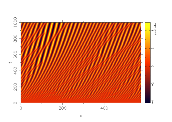
Figure 10: Temporal evolution of the ripples. Note the coarsening and the slowing down of the drift.

The numerical results presented in the figures has been obtained by the integration of Eq. (65) and Eq. (76) using a pseudo-spectral method with $\Delta x=0.1$ and $\Delta t=10^{-5}$ in a system of size $L\sim 30\lambda_{\rm cut-off}$. Figure 10 shows the temporal evolution of the structure corresponding to the case $\nu=\mu=\eta=1$. The simulation has been started from a small amplitude random initial condition. Soon a rather regular pattern appears with wavenumber corresponding to the linearly most unstable mode. The structure contains defects that will trigger the coarsening process: at the end of the simulation the typical wavelength has been doubled. The slowing down of the drift with growing wavelength predicted by Eq. (75) is also clearly observable.

6 Conclusion and discussion

Based on general arguments and observations we have adopted the notion of locality for sand ripple formation. We have then presented general symmetry and conservation considerations to show how a model-independent nonlinear equation for sand ripples can be derived. That equation takes the form

$$h_{t}=-h_{xx}+\nu h_{xxx}+h_{xxxx}+(h_{x}^{2})_{x}+\mu(h_{x}^{2})_{xx}+\eta(h_{x}^{3})_{x}.$$ (78)

The first nonlinearity $(h_{x}^{2})_{x}$ contributes to drift and is not able to saturate the linear growth. So the first efficient nonlinearity is $\mu(h_{x}^{2})_{xx}$. At short time an ordered ripple structure emerges with a wavelength close to that corresponding to the linearly fastest growing mode. Later a coarsening process takes place; With $\eta=0$ coarsening continues indefinitely, until one huge dune is reached. The coarsening is quantified in terms of a dynamical exponent defined in relation to the increase of the mean wavelength, $\lambda\sim t^{1/z}$. We find both analytically and numerically $z=2$. We have also identified that the slope increases in that case without bound when increasing the system size. Thus higher nonlinear terms must become decisive. We have included the next nonlinear term $(h_{x}^{3})_{x}$ which has led to a saturation of the slope (both the height and the wavelength scale in the same manner as a function of the system size). Though at short time this nonlinear term is irrelevant, it dominates dynamics at longer times. Here again we observe a coarsening but with a smaller exponent $1/z=1/4$. The coarsening seems to stop after a certain stage, typically when the wavelength is about twice of the fastest growing mode. We have found that as the ripple structure forms, it drifts sideways. The drift occurs with dispersion (the drift velocity depends on wavelength). The first term which is responsible for the drift is the one proportional to $h_{xxx}$ (note that there is another linear term $h_{x}$ which provides a phase velocity that can be absorbed in $h_{t}$ via a Galilean transformation). The nonlinear term $(h_{x}^{2})_{x}$ though it does not saturate the linear growth it contributes significantly to drift. In particular it can also lead to a drift opposite to the wind. This happens in particular when all three nonlinearities of Eq. (78) are present but $\nu=0$.

The hydrodynamical model captures the full nonlinear equation written above and provides an encouraging physical basis for the derivation of the ripples equation from physical ingredients. Unlike symmetry and conservation laws, the explicit physical model relates the coefficients to the underlying (phenomenological) physical parameters and provides the physical explanation for the initiation of the instability. That instability is also present in a very transparent and general picture in the Anderson’s model.

These two views (explicit phenomenological model and symmetries) have aided in identifying some general picture of the form of the ripple evolution equation. A numerical study, though not exhaustive, has allowed extraction of some general results. It will be of great importance in future studies to quantify experimentally the coarsening process and to identify whether or not the coarsening stops or rather would continue without bounds if energy continues to be injected. This step will be vital to guide further theoretical development.

Figure 1: Different mechanisms of transport of sand: (i) suspension for fine grains (smaller than 100$\mu m$), (ii) saltation and (iii) reptation for grains of intermediate size (between 100 and 200 $\mu m$).

Figure 2: Example front configuration.

Figure 3: Dispersion relation in the framework of Anderson’s model. Real part of the growth rate as a function of the wave number. Full line: spectrum in the case where the reptation length is constant. Dashed line: spectrum in the case where the reptation length is distributed according to a Gaussian law.

Figure 4: Relation of dispersion in the framework of Nishimori-Ouchi model. Real part of the growth rate as a function of the wave number. Full line: above the instability threshold. Dashed line: below the instability threshold.

Figure 5: Dispersion relation $\omega(q)$. The points $q$ and $2q$ show the two modes used in deriving Eq. (67). Note that $\omega(q)>0$ while $\omega(2q)<0$.

Figure 6: Front shape (solid line) for $\nu=0$ and (dashed line) for $\nu=3$.

Figure 7: Amplitudes of the leading Fourier modes of the ripple structure. Thick dashed line shows numerical solution of Eq. (66), thin line shows the far-from-threshold result (Eq. (68)), and dotted line corresponds to the two mode approximation (Eq. (67)).

Figure 8: Temporal evolution of the average wavelength integrating Eq. (65) (pluses) for $\nu=0$, (boxes) for $\nu=1$, and (circles) Eq. (76) with $\nu=\mu=\eta=1$.

Figure 9: Ripple drift velocity $v$ as a function of the ripple wavelength. (Boxes) numerical results from integrating Eq. (65) with $\nu=1$ and (solid line) analytical result for $\lambda/\lambda_{\rm c}\simeq 1$ Eq. (75).

References

- [1] R. A. Bagnold, The Physics of blown sand and desert dunes (Chapmann and Hall, Methuen, London, 1941).
- [2] R. Anderson, Sedimentology 34, 943 (1987).
- [3] Z. Csahók, C. Misbah, and A. Valance, Physica D 128, 87 (1999).
- [4] A. Valance and F. Rioual, Eur. Phys. J. B. 10, 543 (1999).
- [5] R. S. Anderson, M. Sorensen, and B. B. Willets, Acta Mechanica Suppl, 1 (1991).
- [6] D. J. Tritton, Physical Fluid Dynamics, 2nd ed. (Oxford University Press, Oxford, UK, 1988).
- [7] B. R. White and J. C. Schulz, J. Fluid Mech. 81, 497 (1977).
- [8] R. S. Anderson and B. Hallet, Geological Society of American Bulletin 97, 523 (1986).
- [9] S. Mitha, M. Q. Tran, B. T. Werner, and P. K. Haff, Acta Mechanica 63, 267 (1986).
- [10] B. B. Willets and M. A. Rice, Acta Mechanica 63, 255 (1986).
- [11] J. Ungar and P. K. Haff, Sedimentology 34, 289 (1987).
- [12] D. A. Rumpel, Sedimentology 32, 267 (1985).
- [13] B. T. Werner and P. K. Haff, Sedimentology 35, 189 (1988).
- [14] B. T. Werner, Journal of Geology 98, 1 (1990).
- [15] H. Nishimori and N. Ouchi, Phys. Rev. Lett. 71, 197 (1993).
- [16] R. Hoyle and A. Woods, Phys. Rev. E 56, 6861 (1997).
- [17] J.-P. Bouchaud, M. E. Cates, J. R. Prakash, and S. F. Edwards, J. Phys. France I 4, 1383 (1994).
- [18] O. Terzidis, P. Claudin, and J.-P. Bouchaud, Eur. Phys. J. B. 5, 245 (1998).
- [19] P. Politi, Phys. Rev. E 58, 281 (1998).