The Physics of the Glass Transition

Abstract

In this talk, after a short phenomenological introduction on glasses, I will describe some recent progresses that have been done in glasses using the replica method in the definition and in the evaluation of the configurational entropy (or complexity). These results are at the basis of some analytic computations of the thermodynamic glass transition and of the properties below the phase transition point.

1 Introduction

Glasses are roughly speaking liquids that do not crystallize also at very low temperature (to be precise: glasses also do not quasi-crystallize).

These liquids can avoid crystalization mainly for two reasons:

• The liquid does not crystallize because it is cooled very fast: the crystallisation time may become very large at low temperature (e.g. hard spheres at high pressure). The system should be cooled very fast at temperatures near the melting point; however if crystalization is avoided, and the temperature is low enough, (e.g. near the glass transition) the system may be cooled very slowly without producing crystalization.

• The liquid does not crystallize even at equilibrium. An example is a binary mixture of hard spheres with different radius: 50% type A (radius $r_{A}$, 50% type B (radius $r_{A}$, where $R$ denotes $r_{B}/r_{A}$. If $.77<R<.89$ (the bounds may be not precise), the amorphous packing is more dense than a periodic packing, distorted by defects.

Which of the two mechanism is present is irrelevant for understanding the liquid glass transition.

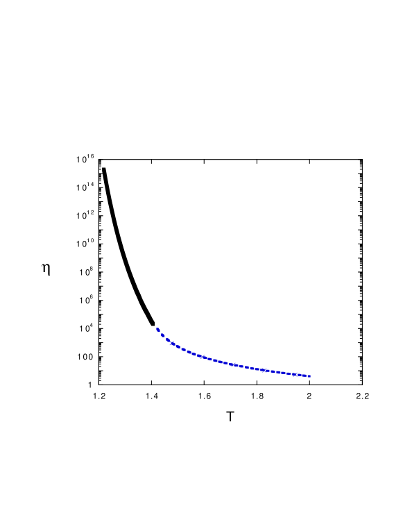
Figure 1: The viscosity as function of the temperature according to the Vogel Fulcher law ($T_{K}=1$ full line) and to the mode coupling theory ($T_{K}=1.375$ dotted line).

Other examples of glassy systems are mixtures: in this case we have $M$ kind of particles and the Hamiltonian of $N$ particles is given by

$$H=\sum_{a,b=1,M}\sum_{i=1,N(a)}\sum_{k=1,N(b)}V_{a,b}\left(x_{a}(i)-x_{b}(k)\right)\ ,$$ (1)

where $a=1,M$; $N(a)=Nc(a)$; $\sum_{a}c(a)=1$. In this case the values of the $N$ concentrations $c$ and the $M(M+1)/2$ functions $V_{a,b}(x)$ describe the model. Well studied case are:

• Soft spheres (non-realistic, but simple), e.g. $M=2$, $c(1)=.5$, $c(2)=.5$, $V_{a,b}(x)=R_{a,b}x^{-12}$.

• Lennard-Jones spheres (more realistic), e.g. $M=2$, $c(1)=.8$, $c(2)=.2$, $V_{a,b}(x)=R_{a,b}x^{-12}-A_{a,b}x^{-6}$.

There are some choices of the parameters which are well studied and in these case it is known that the system does not crystallize, one of these has been introduced by Kob and Anderson in the L-J case and correspond to a particular choice of the parameters $R$ and $A$.

There are many other material which are glass forming, e.g. short polymers, asymmetric molecules (e.g. OTP) …

The behaviour of the viscosity in glass forming liquid is very interesting. We recall that the viscosity can be defined microscopically as follows. We consider a system in a box of large volume $V$ and we call $T_{\mu,\nu}(t)$ the total stress tensor at time $t$. We define the correlation function of the stress tensor at different times:

$$\langle T_{\mu,\nu}(t)T_{\rho,\sigma}(0)\rangle=VS_{\mu,\nu,\rho,\sigma}(t)$$ (2)

One finds, neglecting indices, that $\eta\propto\int dtS(t)\approx\tau^{-\alpha}$, where $\tau$ is the characteristic time of the system (in a first approximation we can suppose that $\alpha=1$).

In fragile glasses the behaviour of the viscosity as function of the temperature can be phenomenological described by the two following regimes:

• In an high temperature region the mode coupling theory is valid: it predicts $\eta\propto(T-T_{c})^{-\gamma}$, where $\gamma$ is not an universal quantity and it a of the orders of a few units.

• In the low temperature region by the Vogel Fulcher law is satisfied: it predicts that $\eta\propto\exp(A(T-T_{K})^{-1})$.

Nearly tautologically fragile glasses can be defined as those glasses that have $T_{K}\neq 0$; strong glasses have $T_{K}\approx 0$.

The glass temperature ($T_{g}$) is the temperature at which the viscosity becomes so large that it cannot be any more measured. This happens after an increase of about 18 order of magnitude (which correspond to a microscopic time changing from $10^{-14}$ to $10^{4}$ seconds): the relaxation time becomes larger than the experimental tine.

A characteristic of glasses is the dependance of the specific heat on the cooling rate. There is a (slightly rounded) discontinuity in the specific heat that it is shifted at lower temperatures when we increase the cooling time.

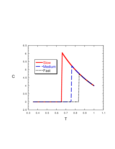
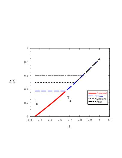
Figure 2: The specific heat and the entropy excess $\Delta S$ for various cooling rates.

For systems that do crystallize if cooled very slowly, one can plot $\Delta S\equiv S(liquid)-S(crystal)$ versus $T$ in the thermalized region. One gets a very smooth curve whose extrapolation becomes negative at a finite temperature. A negative $\Delta S$ does not make sense, so there is a wide spread belief that a phase transition is present before (and quite likely near) the point where the entropy becomes negative. Such a thermodynamic transition (suggested by Kaufmann) would be characterized by a jump of the specific heat. Quite often this temperature is very similar to the temperature found by fitting the viscosity by the Volker Fulcher law and the two temperature are believed to coincide.

Generally speaking it is expected that a thermodynamic phase transition induces a divergent correlation time. However the exponential dependance of the correlation time on the temperature is not so common (in conventional critical slowing down we should have a power like behaviour); moreover an other strange property of the glass transition is the apparent absence of a detectable correlation length or susceptibility (linear or non-linear) which diverges when we approach the transition point.

In section 2, I will firstly present the many valley picture which has been the inspiration point of many works; in the subsequent section I will summarize some of the results that have been obtained using the replica theory on the organization of these valley in phase space, on the temperature dependence of the free energy in each valley, in brief of the free energy landscape. A strategy for applying these ideas to glasses will be presented in section 4 and in the next section I will show some results that have been obtained in the case of a Lennard-Jones binary mixture.

2 The many valleys picture

A quite old statement is that the glass is frozen liquid, which I prefer to reformulate it as that a low temperature a liquid is an unfrozen glass.

Figure 3: An artistic view of a corrugated free energy landscape, the horizontal axis being the configuration space.

The general idea is the following: the phase space of the systems can be approximately decomposed into valleys, labelled by $a$, such that the barrier among these valleys is large in the liquid (in the low temperature region where the viscosity is large) the barriers become infinite at $T_{K}$ [1].

For simplicity I will assume that valleys do maintain their identity when changing the temperature. (in reality they split into smaller valleys when we decrease the temperature [2]). Under this assumption there is a one to one correspondence among valleys and inherent structures, i.e. minima of the Hamiltonian $H$. The properties of the liquid are therefore connected to the properties of the system near the minima of the Hamiltonian.

The partition function can be approximately written as

$$Z=\sum_{a}\exp\left(-\beta Nf_{a}(\beta)\right)\ ,$$ (3)

where $f_{a}(\beta)$ is the free energy density of the $a^{th}$ valley. As we shall see later in the infinite volume limit the previous sum is dominated by those valleys having a given free energy density $f=f^{*}(\beta)$.

The number of relevant valleys at $f=f^{*}(\beta)$ (i.e. ${\cal N}^{*}(\beta)$) is supposed to exponentially increase with the size ($N$) of the system:

$$cN^{*}\approx\exp(N\Sigma^{*}(\beta))\ .$$ (4)

It can be argued that the configurational entropy or complexity $\Sigma^{*}(\beta)$ is approximately near to $\Delta S$: indeed it has suggest long time ago that the configurational entropy $\Sigma^{*}$, goes to zero at the phase transition point [1].

Recently using the techniques stemming from replica theory we have added new ingredients to this old scenario:

• We have construct a microscopic realization of the previous ideas in the mean field models [3, 4]. In other words there are soluble infinite range models in which there is an exponentially large number of valleys and their properties can be computed analytically.

• If we assume that minimal corrections are present in finite dimensions to mean field predictions, the mean field results may be extended to three dimensional glasses.

• The replica method [5] gives tools to do the appropriate computations, both in mean the mean field approach and in short range models.

As outcome of these advances a many valleys picture with detailed predictions on the landscape has been constructed and the properties of glasses can be computed in the framework of replicated liquid theory [6, 7, 8, 9].

3 The free energy landscape

Let us suppose that we can define a temperature free energy functional ($F[\rho]$) as function of the density $\rho(x)$. It is natural to assume that the different valleys are in a first approximation associated to different local minima of this functional, the free energy evaluated at the local minima being the free energy of the corresponding valley.

I will summarize which are in mean field the properties of the local minima the free energy that have been computed explicitly in some long range microscopic models. Although these results have been obtained in some particular models, one can show that they are valid for a quite large class of models (at least in the mean field approximation [10, 11]).

• For $T>T_{c}$ there is one relevant minimum with $\rho(x)=const$. There are many solutions of the equation

  $${\delta F\over\delta\rho}=0.$$ (5)

  which are not minima (there are some negative eigenvalues of the Hessian ${\cal H}(x,y)={\partial^{2}H\over\partial x\partial y}$.

• For $T=T_{c}$ the negative eigenvalues of the Hessian become positive or zero. There is an exponentially large number of minima, connected by flat regions.

• For $T_{c}>T>T_{K}$ the number of relevant minima becomes proportional to $\exp(N\Sigma^{*}(\beta))$. where $\Sigma^{*}(\beta)$ is the configurational entropy or complexity. The minima are separated by barriers that diverge with the number of particles $N$ (in mean field theory), however the barriers are are finite in real life (i.e. beyond mean field theory).

• For $T_{K}>T$ the number of relevant minima is finite. The minima are separated by barriers that diverge with $N$.

For $T_{c}>T>T_{K}$ there is a dual description: the system may be described as a liquid and also as a solid (with an exponentially large number of different solid structures). This duality tell us that all the information needed to study the glass can be extracted from the liquid phase.

4 A more quantitative approach

As we have seen we can write

$$Z(\beta)=\sum_{a}\exp(-\beta Nf_{a}(\beta))=\int d{\cal N}(f,\beta)\exp(-\beta Nf),$$ (6)

where $f_{a}(\beta)$ is the free energy density of the valley labeled by $a$ at the temperature $\beta^{-1}$, and ${\cal N}(f,\beta)$ is the number of valleys with free energy density less than $f$.

We can assume that ${\cal N}(f,\beta)=\exp(N\Sigma(f,\beta))$, where the configurational entropy, or complexity, $\Sigma(f,\beta)$ is positive in the region $f.f_{0}(\beta)$ and vanishes at $f=f_{0}(\beta)$. The quantity $f_{0}(\beta)$ is the minimum value of the free energy: ${\cal N}(f,\beta)$ is zero for $f<f_{0}(\beta)$ [6, 7, 8, 9].

If the equation

$${\partial\Sigma\over\partial f}=\beta$$ (7)

has a solution at $f=f^{*}(\beta)$ (obviously this may happens only for $f^{*}(\beta)>f_{0}(\beta)$), we stay in the liquid phase the free density is given by

$$F=f^{*}-\beta^{-1}\Sigma(f^{*},\beta)$$ (8)

and $\Sigma(f^{*},\beta)=\Sigma^{*}(\beta)$.

Otherwise we stay in the glass phase and

$$F=f_{0}(\beta)\ .$$ (9)

In order to compute the properties in the glass phase we need to know $\Sigma(f,\beta)$: a simple strategy is the following.

We introduce the modified partition function

$$Z(\gamma;\beta)\equiv\exp(-N\gamma\Phi(\gamma;\beta))=\sum_{a}\exp(-\gamma Nf_{a}(\beta)).$$ (10)

Using standard thermodynamical arguments it can be easily proven that in the limit $N\to\infty$ one has:

$$\gamma\Phi(\gamma;\beta)=\gamma f-\Sigma(\beta,f),\ \ \ f={\partial(\gamma\Phi(\gamma;\beta))\over\partial\gamma}.$$

The complexity is obtained from $\Phi(\gamma;\beta)$ in the same way as the entropy is obtained from the usual free energy [12]:

$$\Sigma(\beta,f)={\partial\Phi(\gamma;\beta)\over\partial\gamma}.$$ (11)

A few observations are in order:

• In the new formalism $\gamma$, the free energy and the complexity play respectively the same role of $\beta$, the internal energy and the entropy in the usual formalism.

• In the new formalism $\beta$ only indicates the value of the temperature which is used to compute the free energy and $\gamma$ controls which part of the free energy landscape is sampled.

• When $\beta\to\infty$ we sample the energy landscape:

  $$Z(\gamma;\infty)=\sum_{a}\exp(-\gamma Ne_{a})=\int\nu(e)de\exp(-\gamma Ne)$$ (12)

  where $e_{a}$ are the minima of the Hamiltonian and $\nu(e)$ the density of the minima of the Hamiltonian.

• The equilibrium complexity is given by $\Sigma^{*}(\beta)=\Sigma(\beta;\beta)$. On the other hand $\Sigma(\gamma;\infty)$ give us information on the minima of the Hamiltonian.

It is convenient to write

$$Z(\gamma;\beta)=\int dC\exp\left(-\gamma H(C)-N\gamma f(\beta,C)+N\gamma f(\gamma,C)\right)=$$

$$\int dC\exp\left(-\gamma H(C)-N\gamma\hat{f}(\beta,C)+N\gamma\hat{f}(\gamma,C)\right),$$ (13)

where $\hat{f}(\beta,C)=f(\beta,C)-f(\infty,C)$, $f(\beta,C)$ is is constant in each valley and it is equal to the free energy density of the valley to which the configuration $C$ belongs. and $\hat{f}(\beta,C)$ is the temperature dependent part of free energy density of the valley to which the configuration $C$ belongs.

Our strategy is to use duality and liquid theory to evaluate the properties of $\hat{f}(\beta,C)$.

A simple approximation is the so called quenched approximation which in this case consists in assuming that

$$\exp(-A\hat{f}(\beta,C))\approx\exp(-A\hat{f}_{\gamma}(\beta)),$$ (14)

where $\hat{f}_{\gamma}(\beta)$ is the expectation value of $\hat{f}(\beta,C)$ taken with the probability distribution proportional to $\exp(-\gamma H(C))$.

The quenched approximation would be exact if all the valleys at a given temperature (also with different free energy) would have the same entropy. In other words the fluctuations of the energy are more relevant than the fluctuations of the entropy.

It is now a matter of simple algebra to show that

$$\Phi(\gamma;\beta)=F_{liquid}(\gamma)+\hat{f}_{\gamma}(\beta)-\hat{f}_{\gamma}(\gamma),$$

$$\Sigma(\gamma;\beta)=S_{liquid}(\gamma)-S_{\gamma}(\gamma)+\hat{f}^{\prime}_{\gamma}(\gamma)-\hat{f}^{\prime}_{\gamma}(\beta),$$ (15)

where $\hat{f}^{\prime}_{\gamma}(\beta)={\partial\hat{f}_{\gamma}(\beta)/\partial\gamma}$.

Everything is now computable using liquid theory. Different approximations can be done for $\hat{f}_{\gamma}(\beta)$ and slightly different results may be obtained for the transition temperature and for the specific heat in the glass region. The replica formalism allow us to study directly the function $\Phi(\gamma;\beta)$ and most of the computation are done (for sake of compactness and simplicity) using this powerful tool.

5 Some results

Analytic and numerical computation have been done in many case. I will present here only the results for the Kob Andersen Lennard Jones binary mixture described in the introduction at density $\rho=1.2$.

In order to compute the free energy (or the entropy of the valleys) a simple and useful approximation is to assume that the potential near each minimum of the Hamiltonian is approximately an harmonic one and therefore the free energy of a valley can be computed using an harmonic approximation. In this way one finds that the previous formulae in the liquid phase become

$$\Sigma^{*}(\beta))=S_{liquid}(\beta)-S_{harmonic}(\beta)+\ldots,$$ (16)

where

$$\beta S_{harmonic}=\frac{1}{2}\ln\det\left({\partial^{2}\beta H\over\partial x(i)\partial x(k)}\right).$$ (17)

Similar formulae holds below the transition temperature.

The relevant quantities can be or computed analytically (using liquid theory) or extracted by numerical simulations in the liquid phase.

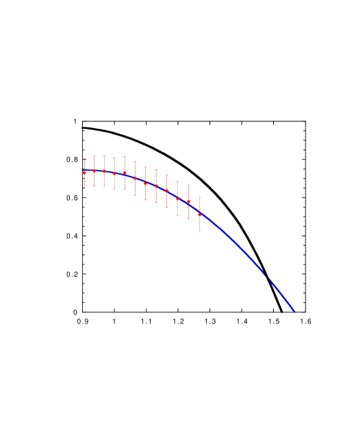
Figure 4: Analytic and numerical complexity as function of $T^{-.4}$.

Both the analytic and the numerical results of [9] for the configurational are shown in fig. 4 (from [9]). The correctness of the numerical estimate have been later confirmed by the more accurate computations of [13].

These microscopic analytic computations support the proposal that there is a thermodynamic liquid glass transition characterized by vanishing of the complexity and that at low temperature below $T_{K}$ the system stays only in a few valleys.

In other words in the glass phase replica symmetry is broken and we aspect that there are characteristic violations of the fluctuation dissipation theorem in off-equilibrium dynamics in the aging regime [14, 15, 16]. Indeed in the aging regime the fluctuation dissipation theorem cannot be applied and generalized dissipation relations are valid. The form of these generalized dissipation relations is fixed by the theory and the resulting predictions are confirmed by numerical simulations.

Direct measurements of these fluctuation dissipation relations in real (not numerical [17]) experiments both for glasses are possible with the present technology. Some experiments are under the way. The outcome will be a crucial test for this theoretical approach and I hope that some results will be available in the next future.

References

- [1] For example see S.Sastry, P. Debenedetti, F.H.Stillinger, Nature 393 554 (1998). K. K. Bhattacharya, K. Broderix, R. Kree, A. Zippelius, cond-mat/9903120. L. Angelani, G. Parisi, G. Ruocco and G. Viliani, Phys. Rev. Lett. 81 4648 (1998)
- [2] A. Barrat, R. Burioni, and M. Mézard, J. Phys. A 29, L81 (1996), A. Barrat, S. Franz and G. Parisi J. Phys. A: Math. Gen. 30, 5593 (1997).
- [3] T.R. Kirkpatrick and D. Thirumalai, Transp. Theor. Stat. Phys. 24, 927 (1995) and references therein.
- [4] A. Crisanti and H.-J. Sommers, J. Phys. I (France) 5, 805 (1995).
- [5] M.Mézard, G.Parisi and M.A.Virasoro, Spin glass theory and beyond, World Scientific (Singapore 1987).
- [6] M. Mézard and G. Parisi, Phys. Rev. Lett. 82 747 (1998); A first principle computation of the thermodynamics of glasses cond-mat 9812180, J. Chem. Phys. in press.
- [7] M. Mézard, How to compute the thermodynamics of a glass using a cloned liquid, cond-mat/9812024, J. Chem. Phys. in press.
- [8] B. Coluzzi, M. Mézard, G. Parisi and P. Verrocchio, Thermodynamics of binary mixture glasses, cond-mat/9903129., J. Chem. Phys. in press
- [9] B. Coluzzi, G. Parisi and P. Verrocchio, Lennard-Jones binary mixture: a thermodynamical approach to glass transition, cond-mat/9904124, J. Chem. Phys, (in press); The thermodynamical liquid-glass transition in a Lennard-Jones binary mixture, cond-mat/9906124, Phys. Rev. Lett. (in press).
- [10] Silvio Franz, Giorgio Parisi Effective potential in glassy systems: theory and simulations, cond-mat/9711215.
- [11] Miguel Cardenas, Silvio Franz, Giorgio Parisi Constrained Boltzmann-Gibbs measures and effective potential for glasses … cond-mat/9801155.
- [12] E. Monasson Phys. Rev. Lett. 75 (1995) 2847.
- [13] W. Kob, F. Sciortino, P. Tartaglia, Inherent Structure Entropy of Supercooled Liquids, cond-mat/9906081.
- [14] L.F. Cugliandolo and J. Kurchan, Phys. Rev. Lett. 71, 173 (1993); J. Phys. A: Math. Gen. 27, 5749 (1994).
- [15] S. Franz and M. Mézard, Europhys. Lett. 26, 209 (1994)
- [16] S. Franz, M. Mézard, G. Parisi and L. Peliti, Phys. Rev. Lett. 81 1758 (1998); The response of glassy systems to random perturbations: a bridge between equilibrium and off-equilibrium, cond-mat/9903370.
- [17] G. Parisi, Phys. Rev. Lett. 79, 3660 (1997).