[

Mobile Bipolaron

Abstract

We explore the properties of the bipolaron in a 1D Holstein-Hubbard model with dynamical quantum phonons. Using a recently developed variational method combined with analytical strong coupling calculations, we compute correlation functions, effective mass, bipolaron isotope effect and the phase diagram. The two site bipolaron has a significantly reduced mass and isotope effect compared to the on-site bipolaron, and is bound in the strong coupling regime up to twice the Hubbard $U$ naively expected. The model can be described in this regime as an effective t-J-V model with nearest neighbor repulsion. These are the most accurate bipolaron calculations to date.

]

While there is a generally accepted belief that in high $T_{c}$ superconductors a dominantly electronic interaction is responsible for the unusually high transition temperatures, the interplay between the electron-phonon interaction and the strong electron-electron interaction nevertheless plays a significant role in determining the physical properties of these strongly correlated systems [1, 2]. Although the study of lattice effects in strongly correlated materials is steadily growing [3, 4, 5, 6, 7], the understanding of the influence of the Hubbard interaction $U$ on bipolaron formation is still incomplete. In particular, it is known that in the strong coupling regime bipolarons have an extremely large effective mass[8, 9], which represents one of the main objections [9, 10] against the theory of small bipolaron superconductivity [11]. Recent calculations in the adiabatic (static phonon) limit show that a first-order phase transition exists between the on-site (S0) and lighter neighboring-site (S1) bipolaron [12]. The properties of the S1 bipolaron were also investigated by variational and exact diagonalization methods [13, 14].

In this letter we present accurate numerical solutions of the Holstein-Hubbard model bipolaron on a 1D infinite lattice. Our results are exact to within the line-widths on the figures in the intermediate and near the strong coupling regimes. The results are compared to analytical calculations in the strong coupling regime.

We consider the Holstein-Hubbard Hamiltonian [15]

$$H =-t\sum_{js}(c_{j+1,s}^{\dagger}c_{j,s}+H.c.)$$ (2)

$$-g\omega\sum_{js}c_{j,s}^{\dagger}c_{j,s}(a_{j}+a_{j}^{\dagger})+\omega\sum_{j}a_{j}^{\dagger}a_{j}+U\sum_{j}n_{j\uparrow}n_{j\downarrow},$$

where $c_{j,s}^{\dagger}$ creates an electron of spin $s$ and $a_{j}^{\dagger}$ creates a phonon on site $j$. The last term in Eq. (2) represents the on-site Coulomb repulsion. We consider the case where two electrons with opposite spins couple to dispersionless optical phonons.

Basis states for the many-body Hilbert space can be written $|M\rangle=|j_{1},j_{2};\dots,n_{m},n_{m+1},\dots,\rangle$, where the up and down electrons are on sites $j1$ and $j2$, and there are $n_{m}$ phonons on site $m$. A variational subspace is constructed beginning with an initial state where both electrons are on the same site with no phonons, and operating repeatedly ($N_{h}$-times) with the off-diagonal pieces ($t$ and $g$) of the Hamiltonian, Eq. (2). All translations of these states are included on an infinite lattice. This method was used previously for the polaron (one electron) [16, 17]. The method is very efficient in the intermediate coupling regime, where it provides results that are variational in the thermodynamic limit and bipolaron energies that are accurate to 7 digits for the case $N_{h}=18$ and size of the Hilbert space $N=2.2\times 10^{6}$ phonon and down electron configurations for a given up electron position.

Before presenting the numerical calculations, we show that many interesting properties of the bipolaron can be found in second-order strong coupling perturbation theory. Following Lang and Firsov[18] we use the canonical transformation $\tilde{H}=e^{S}He^{-S}$, where $S=g\sum_{js}n_{js}(a_{j}-a_{j}^{\dagger})$. The transformed Hamiltonian takes the form

$$\tilde{H} = H_{0}+T$$ (3)

$$H_{0} = \omega\sum_{j}a_{j}^{\dagger}a_{j}-\omega g^{2}\sum_{j}n_{j}+\left(U-2\omega g^{2}\right)\sum_{j}n_{j\uparrow}n_{j\downarrow}$$ (4)

$$T = -te^{-g^{2}}\sum_{js}\left(c_{j+1,s}^{\dagger}c_{j,s}e^{-g\left(a_{j+1}^{\dagger}-a_{j}^{\dagger}\right)}e^{g\left(a_{j+1}-a_{j}\right)}+{\rm H.c.}\right),$$ (5)

where $n_{j}=n_{j\uparrow}+n_{j\downarrow}$. The first term in $H_{0}$ is the energy of the phonon excitations, and the second is the energy gained by displacing the oscillator in the force of the electron. The exponential factors in the $T$ hopping term arise because the Lang-Firsov transformation redefines the origin of the harmonic oscillator when the number of electrons on the site changes. In the limit $g\to 0$ and $\omega\to\infty$ with $\omega g^{2}$ constant, the phonon interaction is instantaneous and the Holstein-Hubbard model maps onto a Hubbard model with an effective Hubbard interaction $\tilde{U}=U-2\omega g^{2}$. In 1D a bound state exists for $\tilde{U}<0$.

In the strong coupling or antiadiabatic limit, $T$ in Eq. (3) is considered a perturbation. It represents the hopping of electrons, including possible creation and destruction of phonon excitations. The S0 state $\phi_{0}=c^{\dagger}_{0\uparrow}c^{\dagger}_{0\downarrow}|0\rangle$ has the lowest energy to zeroth order in $T$ when $\tilde{U}<0$. In perturbation theory to second order, the energy of the S0 bipolaron is

$$E_{bi}^{S0}(k) = U-4\omega g^{2}$$ (6)

$$- {4t^{2}e^{-2g^{2}}\over\omega}\sum_{n=0}{(2g^{2})^{n}\over n!}{(1+(-1)^{n}\cos(k))\over-\tilde{U}/\omega+n}.$$ (7)

The effective mass $m_{S0}^{-1}=\partial^{2}E_{bi}(k)/\partial k^{2}$ can be obtained from Eq. (7) by calculating the infinite sums [8]

$${m_{S0}}^{-1}={4t^{2}\over\omega}e^{-\left(2g^{2}-{\tilde{U}\over\omega}\ln 2g^{2}\right)}\left[\Gamma\left(-{\tilde{U}\over\omega}\right)-\Gamma\left(-{\tilde{U}\over\omega},2g^{2}\right)\right],$$ (8)

where $\Gamma(x)$ and $\Gamma(a,x)$ are the gamma and incomplete gamma functions respectively. Taking the large $g$ limit in Eq. (8), one finds (see also Ref. [8]) $m_{SO}^{-1}\simeq 4\sqrt{\pi}t^{2}\exp(-4g^{2})/(\omega g)$ for $U=0$. At large $g$, $m_{S0}$ is roughly a factor $\exp(3g^{2})$ larger than the polaron mass, $m_{po}^{-1}\simeq 2t\exp(-g^{2})$.

One would naively expect that within the strong coupling approximation, a bipolaron unbinds when $\tilde{U}\geq 0$. This is false: a bound bipolaron may exist even for $\tilde{U}\geq 0$. In this regime, a set of degenerate states $\phi_{i}=c^{\dagger}_{0\uparrow}c^{\dagger}_{i\downarrow}|0\rangle$ for $i\not=0$, written in a translationally invariant form, represents states with minimum energy of $H_{0}$. The energy of a S1 bipolaron is obtained by solving the secular equation $|T_{ij}-\delta_{ij}E_{bi}^{S1}|=0$, where matrix elements $T_{ij}=\langle\phi_{i}|T|\phi_{j}\rangle$ are calculated to second order in $T$.

The main source of binding arises because the second order matrix element $T_{1-1}$ for two neighboring electrons $\mid\uparrow\downarrow\rangle$ to exchange sites is exponentially larger than all other off-diagonal matrix elements. While in the limit $g\to\infty$, $T_{1-1}\propto t^{2}/U$, the second largest (first order) matrix elements $T_{i,i+1}\propto t\exp(-g^{2})$ for $i\neq\{0,-1\}$. The exponential suppression arises from phonon rearrangement whenever the initial and final charge distributions differ. In the singlet configuration, $\phi^{S=0}_{1}=(\phi_{1}+\phi_{-1})/\sqrt{2}$, the diagonal correction to the energy is given by $T_{11}+T_{1-1}$. There is also a contribution to $T_{11}$ that resembles a retardation effect, in which one electron hops creating one or more phonon quanta on its initial site, and the second electron follows absorbing the phonons. This process, however, decreases exponentially with $g$ as $t^{2}\exp(-g^{2})/(\omega g^{2})$, and is not strong enough to bind two polarons in the triplet configuration.

To obtain the S1 bipolaron stability criterion, we note that the secular equation for fixed center of mass momentum $k$ can be mapped onto a tight-binding model for a linear chain. Since all the off-diagonal matrix elements except $T_{1-1}$ scale as $\exp(-g^{2})$, the condition for a bound state is given by $T_{11}+T_{1-1}<T_{ii}$. Keeping only terms of order $t^{2}/(\omega g^{2})$ and setting $k=0$, the matrix elements can be expressed as $T_{11}=T_{a}+T_{b}$, $T_{1-1}=T_{b}$, and $T_{ii}=2T_{a};~{}i>1$, with

$$T_{a} = {-2t^{2}e^{-2g^{2}}\over\omega}\sum_{n=1}{(2g^{2})^{n}\over n!n}\sim-{t^{2}\over\omega g^{2}},$$ (9)

$$T_{b} = {-2t^{2}e^{-2g^{2}}\over\omega}\sum_{n=0}{(2g^{2})^{n}\over n!}{1\over{\tilde{U}\over\omega}+n}\sim-{2t^{2}\over U},$$ (10)

where the final terms refer to the large $g$ limit. In the large $g$ limit, binding occurs for $U<4\omega g^{2}$.

The effective S1 bipolaron mass is computed by approximating the S1 bipolaron wavefunction with only $\phi^{S=0}_{1}$ (omitting the exponential tail),

$$m_{S1}^{-1} \simeq {2t^{2}e^{-2g^{2}}\over\omega}\left[{2\omega\over\tilde{U}}+\sum_{n=1}{g^{2n}\over n!}\left({2\over\tilde{U}/\omega+n}+{1\over n}\right)\right]$$ (11)

$$\sim 2t^{2}e^{-g^{2}}\left[{2\over U-\omega g^{2}}+{1\over\omega g^{2}}\right].$$ (12)

There are three distinct processes contributing to $m_{S1}$: an S1 pair can move by one lattice site through an intermediate doubly occupied state with $n$ phonons (terms that contain $U$ in Eq. (12)), or through an intermediate state with only phonon degrees of freedom (terms without $U$).

The bipolaron isotope effect is a measure of how the bipolaron mass varies with the ion mass $M$, $\alpha\equiv d\ln m_{bi}/d\ln M$. This can also be written $\alpha=-{1\over 2}d\ln m_{bi}/d\ln\omega$, where the derivative is taken with $\omega g^{2}$ held constant. The bipolaron isotope effect $\alpha$ is equal to the superconductivity isotope effect $\alpha_{SC}\equiv-d\ln T_{c}/d\ln M$ only in the low density limit, when superconductivity occurs as a weakly interacting gas of bipolarons Bose condenses. Then in mean field theory (ignoring fluctuations that are important in low dimensions), the transition temperature $T_{c}$ at fixed density is proportional to $m_{bi}^{-1}$, and $\alpha_{SC}=\alpha$. The bipolaron isotope effect is expected to change substantially between the S0 and S1 regimes. Indeed, using Eqs. (8, 12) in the strong coupling limit, we obtain $\alpha_{S0}\sim 2g^{2}-{1\over 4}$ for $U=0$ and $\alpha_{S0}$ decreasing with increasing $U$. In the S1 regime, $\alpha_{S1}\sim g^{2}/2$ and is only weakly dependent on $U$. The bipolaron isotope effect has also been calculated by Alexandrov [19]; the superconductivity isotope effect has been measured by many groups [20].

We now present numerical variational results, using units where hopping $t=1$. Fig. (1) shows the ground state electron-electron density correlation function $C(i-j)=\langle\psi_{o}|n_{i}n_{j}|\psi_{o}\rangle$, where $n_{i}=n_{i\uparrow}+n_{i\downarrow}$. At $g=1$, the bipolaron widens with increasing $U$ and transforms into two unbound polarons (which can only move a finite distance apart in the variational space). The value $U=1.5$ is below the transition to the unbound state at $U_{c}=2.17$, calculated by comparing the polaron and bipolaron energies. At $U=1.5$, $C(i)$ falls off exponentially, while for $U>U_{c}$ the typical distance between electrons is the order of the maximum allowed separation $N_{h}$ [21]. A state of separated polarons is clearly seen for $U=20$.

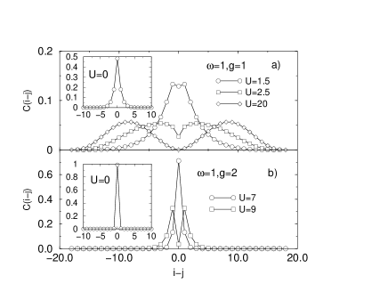
FIG. 1.: Electron-electron correlation function $C(i-j)$ calculated at $\omega=1$, a) $g=1$ and b) $g=2$ for different values of $U$, with $N_{h}=18$. The two ordinate axes have a different range. Insets show results for $U=0$. All curves are normalized, $\sum_{i}C(i)=1$.

Two distinct regimes are seen at $g=2$ within the bipolaronic region. At $U=7<U_{0}\equiv 2\omega g^{2}=8$, the correlation function represents the S0 bipolaron, while at $U=9>U_{0}$ we find the largest probability for two electrons to be on neighboring sites, which is characteristic of the S1 bipolaron. In contrast to previous calculations where phonons were treated classically [12], we find a crossover rather than a phase transition between the two regimes. The precision of presented correlation functions in the bipolaron regime is within the size of the plot symbols in the thermodynamic limit.

Figure (2a) plots the bipolaron mass ratio $R_{m}=m_{bi}/2m_{po}$ vs. $U$ for different values of $\omega$ and $g$. In all cases presented in Fig. (2), $R_{m}$ approaches 1 as $U$ approaches $U=U_{c}$ in agreement with a state of two free polarons. At fixed $\omega=1$ the bipolaron mass ratio increases by several orders of magnitude with increasing $g$ at $U=0$. The increase can be understood within strong coupling theory. Increasing $U$ sharply decreases $R_{m}$ in the S0 regime. Note that the scale in Fig. (2) is logarithmic. Near the strong coupling regime $(g=2)$ and for small $U$, good agreement is found between the numerical and the strong coupling result obtained from Eq. (8). The difference between these results increases as $U$ approaches $U_{0}=8$, where the perturbation theory based on the S0 bipolaron breaks down. In the S1 regime $U>U_{0}$, $R_{m}$ is small, as predicted by the strong coupling result.

FIG. 2.: a) The mass ratio $R_{m}=m_{bi}/2m_{po}$ vs. $U$ and b) the bipolaron isotope effect $\alpha$ vs. $U$. Numerical results are for $N_{h}=18$. Results for $R_{m}$ at $\omega=0.5$ are obtained by extrapolating $N_{h}\to\infty$. Precision in all curves is within the line-width in the thermodynamic limit, except for $\alpha$ with $\omega=0.5$, where the error is estimated to be $\pm 5\%$. The thin line in a) is the strong coupling expansion result for $\omega=1$, $g=2$. Polaron masses in units of the noninteracting electron mass are $m_{po}=1.35,1.76,10.4,3.06$ from top to bottom respectively.

The bipolaron isotope effect, shown in Fig. (2b), is large in the strong coupling ($\omega=1,g=2$) and small $U$ regime, where its value is somewhat below the large $g$ strong coupling prediction $\alpha_{S0}\sim 2g^{2}-{1\over 4}=7.75$. With increasing $U$, $\alpha$ decreases and in the S1 regime approaches $\alpha_{S1}=g^{2}/2=2$. A kink is observed in the crossover regime.

We conclude with the phase diagram $U_{c}(g)$ shown in Fig. (3) at fixed $\omega=1$. Numerical results, shown as circles, indicate the phase boundary between two dissociated polarons each having energy $E_{po}$ and a bipolaron bound state with energy $E_{bi}$. In the inset of Fig. (3) we show the bipolaron binding energy defined as $\Delta=E_{bi}-2E_{po}$. The phase diagram is obtained from $\Delta=0$. The dashed line, given by $U_{0}=2\omega g^{2}$, is a reasonable estimate for the phase boundary at small $g$. At large $g$ the dashed line roughly represents the crossover between a massive S0 and lighter S1 bipolaron. The dot-dashed line is the phase boundary between S1 and the unbound polaron phase, as obtained by degenerate strong coupling perturbation theory. Numerical results approach this line at larger $g$. The dot-dashed line asymptotically approaches $U_{c}=4\omega g^{2}$.

In the S1 regime, the strong coupling expansion can be used to rewrite the Holstein-Hubbard Hamiltonian Eqs. (2,3) as an effective t-J-V model that applies to an arbitrary number of particles,

$$H_{eff} = -t_{1}\sum_{i,s}\tilde{c}^{\dagger}_{i,s}\tilde{c}_{i+1,s}+h.c.+\sum_{i}J{{\bf S}_{i}}{{\bf S}_{i+1}}+Vn_{i}n_{i+1},$$ (13)

where $t_{1}=t\exp(-g^{2})$, $J=-2T_{b}>0$, $V=-T_{a}+T_{b}/2>0$ and $\tilde{c}_{i,s}=c_{i,s}(1-n_{i,-s})$ [22]. The $V$ term is a repulsion between nearest neighbors. For simplicity and in keeping with the approximations used to derive the standard $t-J$ model, we have omitted next-nearest neighbor hopping terms that are of order $t^{2}\exp(-g^{2})/(\omega g^{2})$, and a constant term. While the standard $t-J$ model can be derived from the Hubbard model only for $J<t$, the parameters of $H_{eff}$ are quite different, with $J$ typically much larger than $t_{1}$. In the static limit, an S1 bipolaron is stable in the interval $J/4<V<3J/4$. In the dilute limit, only singlet bipolarons exist with binding energy (in the static limit) $E_{S=0}=-3J/4+V\sim-4t^{2}/U+t^{2}/(\omega g^{2})$, while triplet fluctuations are almost completely frozen out due to the high energy $E_{S=1}=J/4+V$. Such a state is very similar to a negative-$U$ Hubbard model, except that singlets occupy two sites, like in the RVB model.

FIG. 3.: Phase diagram and binding energy $\Delta$ in units of $t$ (inset) calculated at $\omega=1$. Numerical results are circles. For greater accuracy, results near the weak and strong coupling regime were obtained by extrapolating $N_{h}\rightarrow\infty$.

In conclusion, we have demonstrated that near the strong coupling limit a mobile S1 bipolaron exists with an effective mass of the order of a polaron mass, and an isotope effect in the range $0<\alpha<g^{2}/2$. The wavefunction of the S1 bipolaron is a spin singlet with extended $s-$wave spatial symmetry. Taking into account the asymptotic stability criterion $U_{c}=4\omega g^{2}$, it is clear that a triplet S1 bipolaron that corresponds to the $U\to\infty$ solution is not bound. In the static limit, it can be shown that bound states of three or more polarons are not stable in the S1 regime, thus ruling out phase separation. An effective t-J-V model captures the physics of many S1 bipolarons in the strong coupling regime of the Holstein-Hubbard model, where antiferromagnetism is a consequence of the original Hubbard interaction $U$, while the attractive interaction is mediated by phonons. Taking into account the similarity between a system of S1 bipolarons and the negative-U Hubbard model, one should not rule out the possibility that S1 bipolarons form a superconducting state of either $s-$wave or $d-$wave symmetry in two spatial dimensions. In such a state, strong electron-electron interactions and electron-phonon coupling should be treated on an equal footing.

We acknowledge stimulating discussions with V.V. Kabanov and F. Marsiglio. J.B. greatfully acknowledges the support of Los Alamos National Laboratory where part of this work has been performed, and the financial support by the Slovene Ministry of Science. This work was supported in part by the US DOE.

REFERENCES

- [1] Lattice Effects in High- Superconductors, edited by Y. Bar-Yam, T. Egami, J. Mustre de Leon, and A. R. Bishop (World Scientific, Singapore, 1992).
- [2] E.K.H. Salje, A.S. Alexandrov, and W.Y. Liang, Polarons and Bipolarons in High Temperature Superconductors and Related Materials (Cambridge University Press, Cambridge, 1995). A. S. Alexandrov and N. F. Mott, Rep. Progr. Phys. 57, 1197 (1994).
- [3] M. Grilli and C. Castellani, Phys. Rev. B 50, 16880 (1994).
- [4] G. Wellein, H. Röder, and H. Fehske, Phys. Rev. B 53, 9666 (1996).
- [5] F. Marsiglio, Physica C 244, 21 (1995).
- [6] C.H. Pao and H.B. Schüttler, Phys. Rev. B 57, 5051 (1998); 60, 1283 (1999).
- [7] Y. Takada, J. Phys. Soc. Jpn. 65, 1544 (1996).
- [8] A.S. Alexandrov and V.V. Kabanov, Sov. Phys. Solid State 28, 631 (1986).
- [9] E.V.L. de Mello and J. Ranninger, Phys. Rev. B 58, 9098 (1998).
- [10] B.K. Chakraverty, J. Ranninger, and D. Feinberg, Phys. Rev. Lett. 81, 433 (1998).
- [11] A.S. Alexandrov and N.F. Mott, High Temperature Superconductors and other Superfluids (Taylor and Francis, London, 1994); A.S. Alexandrov, V.V. Kabanov, and N.F. Mott, Phys. Rev. Lett. 53, 2863 (1996).
- [12] L. Proville and S. Aubry, Physica D 133, 307 (1998); Eur. Phys. J. B 11, 41 (1999).
- [13] A. La Magna and R. Pucci, Phys. Rev. B 55, 14886 (1997).
- [14] H. Fehske, H. Röder, G. Wellein, and A. Mistriotis, Phys. Rev. B 51, 16582 (1995).
- [15] G. D. Mahan, Many-Particle Physics, Plenum, New York (1981).
- [16] J. Bonča and S. A. Trugman, Phys. Rev. Lett. 75, 2566 (1995).
- [17] J. Bonča, S. A. Trugman and I. Batistič, Phys. Rev. B 60, 1633 (1999).
- [18] I. G. Lang and Yu. A. Firsov, Sov. Phys. JETP 16, 1301 (1963); Sov. Phys. Solid State 5, 2049 (1964).
- [19] A. S. Alexandrov, Phys. Rev. B 46, 14932 (1992).
- [20] See, e.g., G. Zhao, M. B. Hunt, H. Keller, and K. A. Müller, Nature 385, 236 (1997).
- [21] The electrons can be no farther apart than in the variational space, although their center of mass can be anywhere on an infinite lattice.
- [22] A related result was derived by T. Hotta and Y. Takada, Phys. Rev. B 56, 13916 (1997).