Increments of Uncorrelated Time Series Can Be Predicted With a Universal $75\%$ Probability of Success

Abstract

We present a simple and general result that the sign of the variations or increments of uncorrelated times series are predictable with a remarkably high success probability of $75\%$ for symmetric sign distributions. The origin of this paradoxical result is explained in details. We also present some tests on synthetic, financial and global temperature time series.

1 Introduction

Predicting the future evolution of a system from the analysis of past time series is the quest of many disciplines, with a wide range of useful potential applications including natural hazards (volcanic eruptions, earthquakes, floods, hurricanes, global warming, etc.), medecine (epilectic seizure, cardiac arrest, parturition, etc.) and stock markets (economic recessions, financial crashes, investments, etc.). The absolute fundamental prerequisite is that the (possibly spatio-temporal) time series $x_{1},x_{2},...$ possess some dependence of the future on the past. If absent, the best prediction of the future is captured by the mathematical concept of a martingale: the expectation ${\rm E}(x_{t+1}|{\rm past})$ of the future conditioned on the past is the last realisation $x_{t}$. In many applications, one is interested in the variation $x_{t+1}-x_{t}$ of the time series.

The result we present below is, in one sense, obvious and, in another, quite counter-intuitive. Starting from a completely uncorrelated time series, we know by definition that future values cannot be better predicted than by random coin toss. However, we show that the sign of the increments of future values can be predicted with a remarkably high success rate of up to $75\%$ for symmetric time series. The derivation is straightforward but the counter-intuitive result warrants, we believe, its exposition. This little exercice illustrates how tricky can be the assessment of predictive power and statistical testing.

2 First derivation

Consider a time series $x(t)$ sampled at discrete times $t_{1},t_{2},...$ which can be equidistant or not. We denote $x_{1},x_{2},...$ the corresponding measurements. We assume that the measurements $x_{1},x_{2},...$ are i.i.d. (independent identically distributed). Consider first the simple case where $x_{1},x_{2},...$ are uniformly and independently drawn in the interval $[0,1]$ and the average value or expectation is ${\rm E}(x)=1/2$.

2.1 Prediction scheme

We ask the following question: based on previous values up to $x_{i}$, what is the best predictor for the increment $x_{i+1}-x_{i}$? A naive answer would be that, since the $x$’s are independent and uncorrelated, their increments are also independent and the best predictor for the increment $x_{i+1}-x_{i}$ is zero (martingale choice). This turns out to be wrong. If indeed the expectation of the increment is given by

$${\rm E}(x_{i+1}-x_{i})={\rm E}(x_{i+1})-{\rm E}(x_{i})=1/2-1/2=0~,$$ (1)

the conditional expectation ${\rm E}(x_{i+1}-x_{i}|x_{i})$, conditionned on the last realization $x_{i}$, is given by

$${\rm E}(x_{i+1}-x_{i}|x_{i})={\rm E}(x_{i+1}|x_{i})-{\rm E}(x_{i}|x_{i})={1\over 2}-x_{i}~,$$ (2)

where the term $1/2$ uses the independence between $x_{i+1}$ and $x_{i}$ (${\rm E}(x_{i+1}|x_{i})={\rm E}(x_{i+1})=1/2$) and the last term in the r.h.s. uses the identity ${\rm E}(x_{i}|x_{i})=x_{i}$. We thus see that the sign of the increment has some predictability:

• if $x_{i}>1/2$, the expectation is that $x_{i+1}$ will be smaller than $x_{i}$;

• if $x_{i}<1/2$, the expectation is that $x_{i+1}$ will be larger than $x_{i}$.

This predictability can be seen from the fact that the increments of $x(t)$ are anti-correlated:

$${\rm E}\left(\left(x_{i+1}-x_{i}\right)\left(x_{i}-x_{i-1}\right)\right)={\rm E}(x_{i+1}x_{i})-{\rm E}(x_{i+1}x_{i-1})-{\rm E}(x_{i}^{2})+{\rm E}(x_{i}x_{i-1})={1\over 4}-{1\over 4}-{1\over 2}+{1\over 4}=-{1\over 4}~.$$ (3)

This anti-correlation leads indeed to the predictability mentionned above, namely that the best predictor for $x_{i+1}-x_{i}$ is that $x_{i+1}-x_{i}$ be of the sign opposite to $x_{i}-1/2$.

Another way to understand where the predictability of the increments of incorrelated variables comes from is to realize that increments are discrete realizations of the differentiation operator. Under its action, a flat (white noise) spectrum becomes colored towards the “blue” (which is the opposite of the well-known action of integration which “reddens” white noise) and there is thus a short-range correlation appearing in the increments.

2.2 Probability for a successful prediction

A natural question is to determine the success rate $p_{+}$ of this strategy, i.e. the probability that the sign of the increment $x_{i+1}-x_{i}$ be as predicted equal to the sign of $1/2-x_{i}$. To address this question, we study the following quantity

$$\epsilon\equiv{\rm E}\left({\rm sign}\left(x_{i+1}-x_{i}\right){\rm sign}\left({1\over 2}-x_{i}\right)\right)~,$$ (4)

where the product of signs inside the expectation operator is $+1$ if the prediction is born out by the data and $-1$ in the other case. The relationship between $\epsilon$ and $p_{+}$ is

$$\epsilon=(+1)p_{+}+(-1)(1-p_{+})=2p_{+}-1~~~\to~~~p_{+}={1\over 2}+{\epsilon\over 2}~.$$ (5)

Expression (5) shows that $\epsilon$ quantifies the deviation for the random coin toss result $p_{+}=50\%$. From the definition (4), we have

$$\epsilon=\int_{0}^{1\over 2}dx_{i}~(+1)\left(\int_{0}^{x_{i}}dx_{i+1}~(-1)+\int_{x_{i}}^{1}dx_{i+1}~(+1)\right)+\int_{1\over 2}^{1}dx_{i}~(-1)\left(\int_{0}^{x_{i}}dx_{i+1}~(-1)+\int_{x_{i}}^{1}dx_{i+1}~(+1)\right)~,$$ (6)

which gives

$$\epsilon=1/2~~~~~{\rm and~thus}~~~~p_{+}=75\%~.$$ (7)

Figure 1 shows a numerical simulation which evaluates $p_{+}$ as a function of cumulative number of realisations with the strategy that $x_{i+1}-x_{i}$ is predicted of the opposite sign to $x_{i}-1/2$, using a pseudo-random number generator with values uniformely distributed between $0$ and $1$.

3 General derivation for arbitrary distributions

This result is actually quite general. Consider an arbitrary random variable $x_{i}$ with arbitrary probability density distribution $P(x)$ with average $\langle x\rangle$. We form the centered variable

$$\delta_{i}\equiv x_{i}-\langle x\rangle$$ (8)

with zero mean $\langle\delta\rangle=0$ and pdf $P(\delta)$. Similarly to (2), we study the conditional expectation of its increments $\delta_{i+1}-\delta_{i}$, given the last realization $\delta_{i}$:

$${\rm E}(\delta_{i+1}-\delta_{i}|\delta_{i})={\rm E}(\delta_{i+1}|\delta_{i})-{\rm E}(\delta_{i}|\delta_{i})=-\delta_{i}~,$$ (9)

where we have used the fact that the $\delta_{i}$’s are uncorrelated. Thus, the best predictor of the sign of the increment of the $\delta$’s is the opposite of the sign of the last realization. We then quantify the probability of prediction success through the quantity defined similarly to (4) as

$$\epsilon\equiv-{\rm E}\left({\rm sign}\left(\delta_{i+1}-\delta_{i}\right){\rm sign}\left(\delta_{i}\right)\right)~,$$ (10)

which is related to the success probability $p_{+}$ by (5). It is easily calculated as

$$\epsilon = \int_{-\infty}^{0}d\delta_{i}~P(\delta_{i})~(+1)\left[\int_{-\infty}^{\delta_{i}}d\delta_{i+1}~P(\delta_{i+1})~(-1)+\int_{\delta_{i}}^{+\infty}d\delta_{i+1}~P(\delta_{i+1})~(+1)\right]$$ (11)

$$+ \int_{0}^{+\infty}d\delta_{i}~P(\delta_{i})~(-1)\left[\int_{-\infty}^{\delta_{i}}d\delta_{i+1}~P(\delta_{i+1})~(-1)+\int_{\delta_{i}}^{+\infty}d\delta_{i+1}~P(\delta_{i+1})~(+1)\right]~.$$

It is convenient to introduce the cumulative distribution

$$F(x)\equiv\int_{-\infty}^{x}d\delta~P(\delta)~,$$ (12)

and the probabilities $F_{-}=F(0)$ (resp. $F_{+}=1-F(0)$) that $\delta$ be less (resp. larger) than $0$. Expression (11) transforms into

$$\epsilon=F_{-}-F_{+}-\left(F(0)\right)^{2}+\left(F(+\infty)\right)^{2}-\left(F(0)\right)^{2}~,$$ (13)

where we have used the identity $2\int_{-\infty}^{y}dx~P(x)~F(x)=[F(y)]^{2}$. Using the definition of $F_{-}$ and $F_{+}$ and the normalization $F(+\infty)=1$ leads to

$$\epsilon=2F_{+}(1-F_{+})~~~~~{\rm and}~~~~~p_{+}={1\over 2}+F_{+}(1-F_{+})~.$$ (14)

For symmetric distributions and for those distributions such that $F_{+}=1/2$, we retrieve the previous result (7). This result is thus seen to be very general and independent of the shape of the distribution of the i.i.d. variables as long as $F_{+}=1/2$ (attained in particular but not exclusively for symmetric distributions). Note that the value $p_{+}=75\%$ is the largest possible result attained for $F_{+}=1/2$. For $F_{+}\neq 1/2$, $0.5\leq p_{+}<0.75$.

Figure 2 shows the estimation of $p_{+}$ used on the thirty year US treasury bond TYX from Oct. 29, 1993 till Aug. 9, 1999. Specifically, we start from the daily close quotes $q(t)$ and construct the price variations $\delta q(t)=q(t)-q(t-1)$. We try to predict the variation of $\delta q(t)$ with the strategy that $\delta q(t+1)-\delta q(t)$ is predicted of the opposite sign to $\delta q(t)-\langle\delta q\rangle$. The corresponding success probability $p_{+}$ is plotted as a function of time by cumulating the realizations to estimate $p_{+}$. As expected, at the beginning, large fluctuations express the limited statistics. As the statistics improves, $p_{+}$ converges to the predicted value $75\%$. We note that, in comparison to the pseudo-random number series shown in figure 1, the convergence seems to occur at a similar rate, suggesting that there are no appreciable global short-range correlations, in agreement with many previous statistical tests [1, 2, 3].

4 Discussion

This paradoxical result tells us that one can get on average a success rate of three out of four in guessing what is the sign of the increment of uncorrelated random variables. This is quite surprising a priori but, as we explained above, stems from the action of the differential operator which makes the spectrum “blueish”, thus introducing short-range correlations.

This predictive skill does not lead to any anomalies. Consider for instance the time series of price returns of a stock market. According to the efficient market hypothesis (ref.[1] and references therein) and the random walk model, successive (say daily) price returns of liquid organized markets are essentially independent with approximately symmetric distributions. Our result (14) shows then that we can predict with a $75\%$ accuracy the sign of the increment of the daily returns (and not the sign of the returns that are proportional to the increment of the prices themselves). This predictive skill is not associate to an arbitrage opportunities in market trading. This can be seen as follows. For simplicity of language, we consider price returns $\delta$’s relative to their average so that we deal with uncorrelated variables with zero mean as defined in (8). In addition, we restrict our discussion to the optimal case where $F_{+}=1/2$. Consider first the situation where $\delta_{i}$ is positive and quite large (say two standard deviations above zero). We expect that any typical realization, and in particular the next one $\delta_{i+1}$, to be positive or negative but close to zero to within say one standard deviation. This implies that we expect with a large probability $\delta_{i+1}$ to be smaller than $\delta_{i}$. This is the guess that is compatible and in fact constructs the result (14). Consider now the second situation where $\delta_{i}$ is positive but very small and close to zero. We then have by construction of the process that $\delta_{i+1}$ will be larger or smaller than $\delta_{i}$ with probability close to $1/2$. In this case, we loose any predictive skill. What the result (14) quantifies mathematically is that all these types of realizations averages out to a global probability of $75\%$ for the sign of the increment to be predicted by the sign of $-\delta_{i}$. This large value is not giving us any “martingale” (in the common sense of the word). Actually, it states simply that, for independent realizations, large values have to be followed by smaller ones. This analysis relies fundamentally on the independence between successive occurrence of the variables $\delta_{i}$. Predicting with $75\%$ probability the sign of $\delta_{i+1}-\delta_{i}$ does not improve in any way our success rate for prediction the sign of $\delta_{i+1}$ (which would be the real arbitrage opportunity).

Deviations from $p_{+}=75\%$, and in particular results larger than $75\%$ which is a maximum in the uncorrelated case (see (14), signal the presence of correlations. An instance is shown in figure 3 which plots $p_{+}$ for the prediction of the variations of the isotopic deuterium time series from the Vostok (south Pole) ice core sample, which is a proxy for the local temperature from about 220 ky in the past to present. The data is taken from [4]. We observe that $p_{+}$ remains above $75\%$ showing a significant genuine anti-correlation.

Acknowledgements: We thank P. Yiou for providing the temperature time series and S. Gluzman for stimulating discussions.

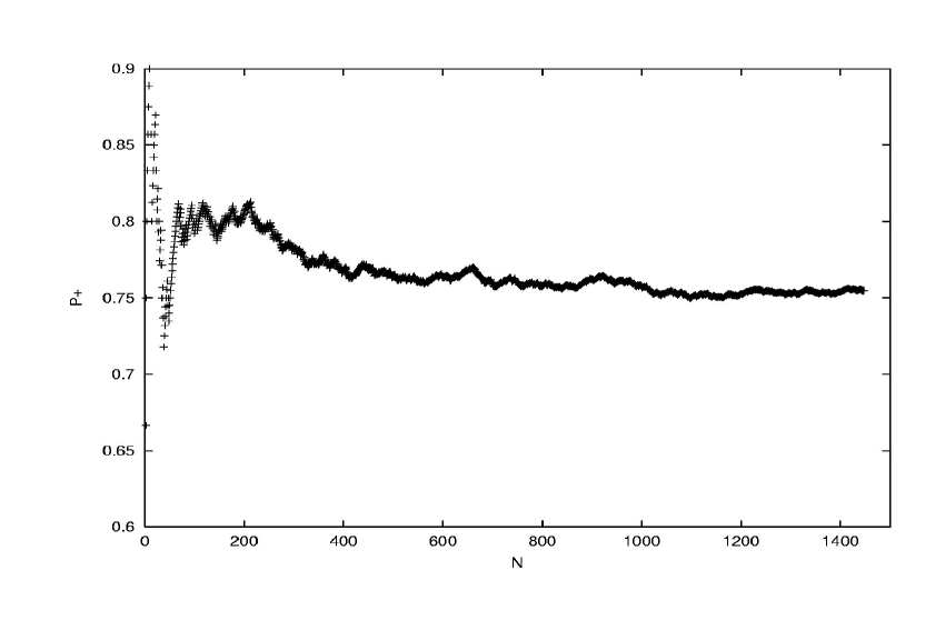
Figure 1: Numerical simulation which evaluates $p_{+}$ as a function of cumulative number of realisations with the strategy that $x_{i+1}-x_{i}$ is predicted of the opposite sign to $x_{i}-1/2$, using a pseudo-random number generator with values uniformely distributed between $0$ and $1$.

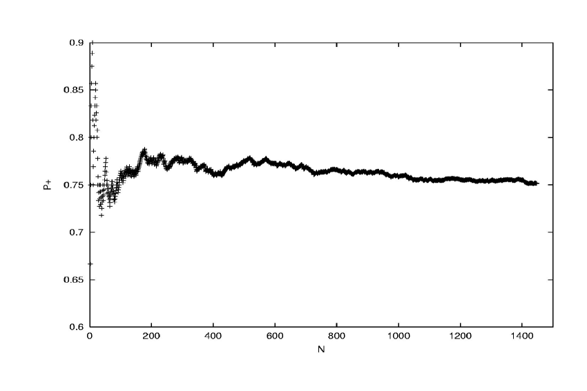
Figure 2: Predictability of the increments of the price variations, i.e. the acceleration, of the thirty year US treasury bond TYX from Oct. 29, 1993 till Aug. 9, 1999. Specifically, we start from the daily close quotes $q(t)$ and construct the price variations $\delta q(t)=q(t)-q(t-1)$. We try to predict the variation of $\delta q(t)$ with the strategy that $\delta q(t+1)-\delta q(t)$ is predicted of the opposite sign to $\delta q(t)-\langle q\rangle$. The corresponding success probability $p_{+}$ is plotted as a function of time by cumulating the realizations to estimate $p_{+}$.

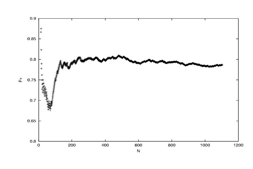
Figure 3: Success probability $p_{+}$ for the prediction of the variations of the isotopic deuterium time series from the Vostok (south Pole) ice core sample, which is a proxy for the local temperature from about 220 thousand years in the past to present. The data is taken from [4].

References

- [1] J.Y. Campbell, A.W. Lo and A.C. MacKinlay, The econometrics of financial markets (Princeton, N.J. : Princeton University Press, 1997).
- [2] J.P. Bouchaud and M. Potters, Théory des risques financiers (Aléa Saclay, 1997).
- [3] R. N. Mantegna and H. E. Stanley, Introduction to Econophysics: Correlations & Complexity in Finance (Cambridge University Press , Cambridge, 1999).
- [4] J. Jouzel, N.I. Barkov, J.M. Barnola, M. Bender et al., Extending the Vostok ice-core record of paleoclimate to the penultimate glacial period, Nature 364, N6436:407-412 (1993).