Density-Matrix Renormalization-Group Analysis of Quantum Critical Points:
I. Quantum Spin Chains

Abstract

We present a simple method, combining the density-matrix renormalization-group (DMRG) algorithm with finite-size scaling, which permits the study of critical behavior in quantum spin chains. Spin moments and dimerization are induced by boundary conditions at the chain ends and these exhibit power-law decay at critical points. Results are presented for the spin-$1/2$ Heisenberg antiferromagnet; an analytic calculation shows that logarithmic corrections to scaling can sometimes be avoided. We also examine the spin-$1$ chain at the critical point separating the Haldane gap and dimerized phases. Exponents for the dimer-dimer and the spin-spin correlation functions are consistent with results obtained from bosonization.

I Introduction

Quantum critical points are characterized by fluctuations over all length and time scales and by the appearance of power law scaling. In this paper we present a simple but powerful numerical method to access quantum critical points in one-dimensional systems. The method combines the density-matrix renormalization-group (DMRG) algorithm and finite-size scaling ideas. We illustrate the method by applying it to several well-understood quantum spin chains. In a second paper to follow we apply the method to new classes of supersymmetric spin chains which describe various disordered electron systems[1].

The development of the density-matrix renormalization-group (DMRG) algorithm by White[2] represented an important improvement over previous numerical methods for the study of low dimensional lattice models. It has been applied to a wide variety of systems[3]. The DMRG approach was first used to study the ground state properties and low-energy excitations of one-dimensional chains. It has been extensively applied to the study of various spin chains. Low-lying excited states of the spin-$1$[4, 5, 6] and spin-$1/2$[7] Heisenberg antiferromagnets have been calculated. Likewise, spin-$1$ chains with quadratic and biquadratic interactions[8, 9], a spin-$2$ antiferromagnetic chain[10, 11], spin-$1/2$ and spin-$1$ chains with dimerization and/or frustration (next-nearest-neighbor coupling)[12, 13, 14, 15, 16], and frustrated spin-$3/2$ and spin-$2$ chains[17] have all been studied. Edge excitations[6, 10, 18, 19] at the ends of finite spin chains and the effects of perturbations such as a weak magnetic field coupled to a few sites[20] have been considered. Randomness in the form of random transverse magnetic field in a spin-$1/2$ XY model[21], random exchange couplings[22], and random modulation patterns of the exchange[23, 24], has been examined. Finally, alternating spin magnitudes[25], the presence of a constant[26] or a staggered[27] magnetic field in a spin-$1$ chain, bond doping[28], the effects of a local impurity[29], and interactions with quantum phonons[30, 31] have also been considered.

Most of the above work involves systems in which the first excited state is separated from the ground state by a non-zero energy gap as the DMRG works best for gapped systems. First attempts to extract critical behavior of gapless systems used the DMRG to generate renormalization transformations of the coupling constants in the Hamiltonian[32, 33]. Hallberg et al.[34] studied the critical behavior of $S=1/2$ and $S=3/2$ quantum spin chains with periodic boundary conditions through extensive calculations of ground state correlation functions at different separations and different chain sizes $L$. Spin correlation functions in an open chain have also been calculated and compared with results calculated from low-energy field theory, showing that estimates of the amplitudes can also be obtained[35]. The approach described in this paper was applied to the spin-$1/2$ Heisenberg chain and a non-Hermitian supersymmetric (SUSY) spin chain[36]. More recently, critical behavior of classical one-dimensional reaction-diffusion models[37] and the two-dimensional Potts model[38] has been studied using the finite-size DMRG algorithm. Bulk and surface exponents of the Potts and Ising model have been obtained by using the DMRG to calculate correlation functions at different separations and collapsing curves obtained at different system sizes[39]. The SUSY chain describing the spin quantum Hall effect (SQHE) plateau transition was also examined in some detail. Critical exponents were extracted[40] and compared to exact predictions[41]. Thermodynamic properties of other two-dimensional classical critical systems have also been studied by the DMRG method[42, 43, 44]. Finally, Andersson et al. investigated the convergence of the DMRG in the thermodynamic limit for a gapless system of non-interacting fermions[45].

The method described in this paper combines the DMRG algorithm with finite-size scaling analysis, and yields accurate critical exponents. The main advantage of the method is its simplicity. Only the calculation of ground state correlations near the middle of chains with open boundary conditions are required. The relatively simple “infinite-size” DMRG algorithm[2] is particularly accurate for this job. In Sec. II we describe the method. The tight-binding model can be solved exactly and in Sec. III we use it to illustrate our scaling analysis. DMRG results are presented in Sec. IV for the anisotropic $S=1/2$ Heisenberg antiferromagnet and several critical exponents are obtained. An analytical calculation shows that multiplicative logarithmic corrections – which complicate the extraction of accurate critical exponents – may be avoided in some instances. In Sec. V, the $S=1$ antiferromagnetic spin chain is studied, focusing on the critical point that separates the Haldane and the dimerized phases. We conclude with a summary in Sec. VI.

II The DMRG / Finite-Size Scaling Approach

We first describe how critical exponents may be obtained from a finite-size scaling analysis of chains with open or fixed boundary conditions. These boundary conditions are the simplest to implement in DMRG calculations. In the next subsection the DMRG algorithm itself is briefly described.

A Finite-Size Scaling

To illustrate the sorts of power-law scaling we wish to examine, first consider the case of a spin chain with periodic boundary conditions that is at its critical point. The system can be moved away from criticality by turning on a uniform magnetic field, say in the x-direction, at each site:

$$H_{B}=h~{}\sum_{j=1}^{L}S^{x}_{j}\ .$$ (1)

This perturbation makes the correlation length finite:

$$\xi_{B}~{}\propto~{}|h|^{-\nu_{B}}\ .$$ (2)

Explicit dimerization, breaking the symmetry of translation by one site, also moves the system away from criticality. For a Heisenberg antiferromagnet, this can be realized by the addition of a staggering term $R$ to the Hamiltonian:

$$H=\sum_{j=1}^{L-1}[1+(-1)^{j}R]~{}\vec{S}_{j}\cdot\vec{S}_{j+1}\ .$$ (3)

The correlation length $\xi$ in this case scales as

$$\xi~{}\propto~{}|R|^{-\nu}\ .$$ (4)

Thus there are two independent exponents which correspond to these two perturbations of critical spin chains. Two-parameter scaling functions can be written for various observables and, for a finite system, these involve two dimensionless variables: the ratios $L/\xi$ and $L/\xi_{B}$. The induced dimerization, defined for now as the modulation of the $x-x$ and $y-y$ spin-spin correlations on even versus odd links,

$$\Delta=(-1)^{j}~{}\left[\langle S^{x}_{j}S^{x}_{j+1}+S^{y}_{j}S^{y}_{j+1}\rangle-\langle S^{x}_{j-1}S^{x}_{j}+S^{y}_{j-1}S^{y}_{j}\rangle\right]\ ,$$ (5)

is of course independent of the site index for periodic chains, and scales as a function of the chain length $L$, the field $h$, and the dimerization parameter $R$ as:

$$\Delta(L,R,h)={\rm sgn}(R)~{}|R|^{\alpha_{\Delta}}~{}f_{\Delta}(L|R|^{\nu},L|h|^{\nu_{B}})\ .$$ (6)

When the applied magnetic field is removed, $h=0$, and this expression simplifies to:

$$\Delta(L,R) = {\rm sgn}(R)~{}|R|^{\alpha_{\Delta}}~{}g_{\Delta}(L|R|^{\nu})$$ (7)

$$\sim L^{x_{\Delta}}~{}R~{}~{}~{}~{}{\rm as}~{}~{}~{}R\rightarrow 0,$$ (8)

where the second line follows from the fact that when the perturbation $R$ is very small, or equivalently when the correlation length is larger than the system size, the net induced dimerization must be an analytic, linear, function of $R$. Therefore, for $|x|\ll 1$, the scaling function $g_{\Delta}(x)$ is given by:

$$g_{\Delta}(x)=|x|^{-\alpha_{\Delta}/\nu}~{}(a_{1}|x|^{1/\nu}+a_{2}|x|^{2/\nu}+\ldots);$$ (9)

the first term yields linear dependence of $\Delta$ in $R$ in the $R\rightarrow 0$ limit, in agreement with Eq. 8, and the subsequent terms are higher order corrections. To recover the correct $L$-dependence, we must set

$$x_{\Delta}={{1-\alpha_{\Delta}}\over{\nu}}\ .$$ (10)

The exponent $x_{\Delta}$ and the correlation length exponent $\nu$ satisfy the usual relation

$$\nu={{1}\over{2-x_{\Delta}}}\ .$$ (11)

The applied magnetic field also polarizes the spins along the chain. The scaling form for the spin moment at each site is given by:

$$\langle S^{x}\rangle={\rm sgn}(h)~{}|h|^{\alpha_{B}}~{}f_{B}(L|R|^{\nu},L|h|^{\nu_{B}})\ .$$ (12)

With no applied dimerization, $R=0$, and we expect the simple power-law:

$$\langle S^{x}\rangle\sim L^{x_{B}}~{}h~{}~{}~{}~{}{\rm as}~{}~{}~{}h\rightarrow 0\ .$$ (13)

Therefore, $x_{B}=(1-\alpha_{B})/\nu_{B}$.

Alternatively, dimerization can be induced by open boundary conditions, and we take advantage of this fact to extract critical exponents. As depicted in Fig. 1, open boundary conditions favor enhanced nearest-neighbor spin-spin correlations on the two outermost links. Chains of increasing length $L=4,6,8,\ldots$ exhibit alternating patterns of dimerization on the interior bonds. Likewise, spin moments may be induced in the interior of the chain by applying a magnetic field to the ends of the chain. Strong applied edge magnetic fields completely polarize the end spins and induce non-zero and alternating spin moments along the chain. Alternatively, spin moments can be induced as before by a staggered magnetic field applied along the entire chain. Here however we consider only edge magnetic fields.

FIG. 1.: Extraction of critical behavior from finite-size effects. Dimerization of the nearest-neighbor spin-spin correlation function, indicated here by alternating strong (solid) and weak (dashed) bonds, is induced by the open boundary conditions. Spin moments are induced by the application of a magnetic field of strength $\pm h$ to the two spins at the ends of the chains.

We monitor the induced dimerization and spin moments at the center of the chain as the chain length $L$ is enlarged via the DMRG algorithm. This scaling analysis is convenient because the relatively simple infinite-size DMRG algorithm applies to open chains and is most accurate at the center region of the chain where we focus our attention. The induced dimerization and spin moments in the interior of the chain show power-law scaling at the critical point[46]. Igloi and Rieger demonstrated power-law scaling for a variety of open boundary conditions (free, fixed and mixed)[47]. At the critical point $R=0$ and $h=0$ the induced dimerization scales as a power-law with possible multiplicative logarithmic corrections:

$$\Delta(L/2)=L^{-x_{\Delta}}~{}(\ln L)^{y_{\Delta}}~{}\big{(}a+\frac{b}{L}+\ldots\big{)}\ .$$ (14)

A similar expression holds for the induced spin moment at the center of the chain, $\langle S^{x}(L/2)\rangle$, with the replacement of the exponents $x_{\Delta}\rightarrow x_{B}$ and $y_{\Delta}\rightarrow y_{B}$.

B Infinite-Size DMRG Algorithm

The name “density-matrix renormalization-group” is something of a misnomer as the method is most accurate away from critical points, when there is an energy gap for excitations. It is helpful to think of the DMRG algorithm as a systematic variational approximation for the calculation of the ground state and/or low-lying excitations, principally in one dimension. The Hilbert space of a quantum chain generally grows exponentially with the chain length, and eventually must exceed available computer memory. The DMRG algorithm is an efficient way to truncate the Hilbert space; as the size of the space retained can be varied (up to machine limits) it is possible to ascertain the size of errors introduced by the truncation.

For simplicity, we use the so-called “infinite-size” DMRG algorithm[2]. As the algorithm has been described in some detail by White, we just sketch the essentials of the method. It begins with the (numerically exact) diagonalization of an open chain consisting of just four sites, each site having on-site Hilbert space of dimension $D$. For quantum spin chains $D=2S+1$, thus $D=2$ for the spin-1/2 Heisenberg antiferromagnet. The chain is then cut through the middle into two pieces, one half of which is interpreted as the “system” and the other half as the “environment,” the two parts combined being thought of as the entire “universe” of the problem, see Fig. 2. At this point the reduced density matrix for the system, of size $DM\times DM$ is constructed by performing a partial trace over the environment half of the chain. It is defined by:

$$\rho_{ij}=\sum_{i^{\prime}=1}^{DM}\Psi_{ii^{\prime}}\Psi_{ji^{\prime}},$$ (15)

where $\Psi_{ii^{\prime}}=\langle ii^{\prime}|\Psi\rangle$ are the real-valued matrix elements of the eigenstate of interest (the “target” which is often the ground state) projected onto a basis of states labeled by unprimed Roman index $i$ which covers the system half of the chain and primed index $i^{\prime}$ which covers the environment half of the chain. The eigenvalues of the reduced density matrix are real, positive, and sum up to one; these are interpreted as probabilities. We keep only the $M$ most probable eigenstates corresponding to the largest eigenvalues, and discard the remaining $M(D-1)$ eigenstates. The retained states form a new basis for the problem. Next, two new sites are added to the middle of the chain and the pieces are connected, yielding a chain of size $L=6$. The process is then repeated by finding the targeted state of this chain, constructing the new reduced density matrix and again projecting onto the $M$ most probable states. As the chain length grows in steps of two, the total Hilbert space dimension grows by a multiplicative factor of $D^{2}$. None of the Hilbert space is thrown away until the chain grows large enough that its Hilbert space exceeds the space that is held in reserve, in other words until $D^{L}>D^{2}M^{2}$. The truncation process damages the outer regions of the chain the most, and the central region is treated most accurately.

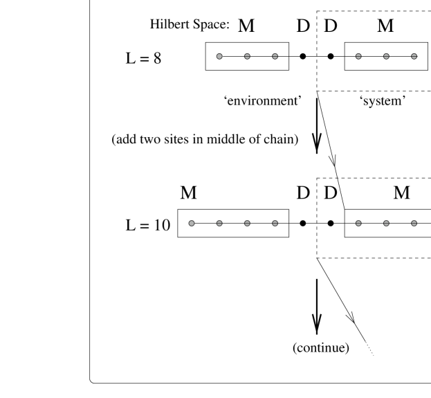
FIG. 2.: Schematic of one iteration in the infinite-size DMRG algorithm. At each step, a “new block” is formed for each half of the chain (the “old block” plus one additional site) and two more sites are added in the middle of the chain, increasing its length by two.

One advantage of the method presented in this paper is that critical exponents are extracted from ground-state correlations only. Excited states are not needed for these exponents and there is no need to calculate the excitation gap. Furthermore, the finite size analysis described in the previous subsection takes advantage of the fact that the DMRG algorithm works best with open chains and treats the central region of the chain most accurately. The use of the more complicated finite-size algorithm might yield even more accurate results. However, we show below that we can calculate critical exponents to an accuracy of a few percent or better with the infinite-size algorithm.

III Tight Binding Model at Half-Filling

As a simple first illustration of our finite-size scaling method we study the ordinary tight binding model of spinless fermions hopping from site-to-site along a chain at half-filling. Obviously, the DMRG algorithm is not needed in this case as we can solve the quadratic problem exactly via a Fourier transform. Due to particle-hole symmetry, at half-filling the chemical potential is zero. The correlation length exponent for this system is $\nu=1$. A direct way to see this is by introducing the staggering parameter $R$ to modulate the amplitude of the hopping matrix elements on even versus odd links:

$$H = t\sum_{j=0}^{L-1}[1+(-1)^{j}R]\big{(}c^{\dagger}_{j}c_{j+1}+h.c.\big{)}\ .$$ (16)

To diagonalize the Hamiltonian, in the case of periodic boundary conditions $c_{0}=c_{L}$, we introduce separate fermion operators for even and odd sites as follows:

$$c_{2j}=d_{2j}$$ (17)

$$c_{2j-1}=e_{2j}$$ (18)

After the Fourier transformation to momentum-space, the Hamiltonian can be written as:

$$H=t\sum_{k}\bigg{\{}[(1-R)+e^{2ik}(1+R)]~{}d_{k}^{\dagger}e_{k}+[(1-R)+e^{-2ik}(1+R)]~{}e^{\dagger}_{k}d_{k}\bigg{\}},$$ (19)

where the lattice spacing $a=1$. For each $k$, diagonalization of the $2\times 2$ matrix yields the dispersion relation:

$$\epsilon_{k}=\pm 2t\sqrt{1-(1-R^{2})\sin^{2}(k)}.$$ (20)

At half-filling the ground state has all states with $\epsilon_{k}<0$ occupied. The left and right Fermi points are, respectively, $k_{F}=\pm\pi/2$. Hence the gap $m=2t|R|$. As the correlation length $\xi\propto m^{-1}\propto|R|^{-1}$ we obtain $\nu=1$. Since $\nu^{-1}=2-x_{\Delta}=1$, the dimerization exponent $x_{\Delta}=1$.

We now reproduce this result using the finite-size scaling method applied to open chains. We consider a finite chain of length $L$ with open boundary conditions and calculate the induced dimerization $\Delta(j)=(-1)^{j}~{}\langle c^{\dagger}_{j}c_{j+1}-c^{\dagger}_{j+1}c_{j+2}\rangle$ around the chain center $j=L/2$, and extract its leading dependence on $L$. Open boundary conditions are imposed by using the Fourier transform

$$c_{j} = \frac{1}{\sqrt{2(L+1)}}\sum_{m=1}^{L}c_{k_{m}}~{}(e^{ik_{m}j}-e^{-ik_{m}j}),$$ (21)

$$k_{m} = \frac{\pi}{L+1}m,\hskip 28.45274ptm=1,2,\ldots,L$$ (22)

as this enforces $c_{0}=c_{L+1}=0$. Filling all of the negative energy states at half-filling, the expectation value of the dimerization at $L/2$ can be found by straightforward calculation:

$$\Delta(L/2)\propto\frac{1}{L+1}\sum_{m=\frac{L}{2}+1}^{L}\big{[}\cos[k_{m}(L+3)]-\cos[k_{m}(L+1)]\big{]}.$$ (23)

This sum can be evaluated numerically with the result that $x_{\Delta}\rightarrow 1$ as $L\rightarrow\infty$ as shown in Fig. 3, in agreement with the explicit calculation for the periodic chain. It is also easy to show that open chains with an odd number of sites have vanishing induced dimerization at the center of the chain, as expected by the symmetry of reflection about the central site.

FIG. 3.: Induced dimerization in the tight binding model. A log-log plot of the dimerization at the center of the chain (Eq. 23) is shown as a function of the chain length $L$. For more complicated systems, the DMRG algorithm is employed to calculate $\Delta(L/2)$ numerically. In the inset, the dimerization exponent calculated from the slope of the curve shown in the main graph is plotted as function of $1/\ln(L)$. For small $L$ there are subleading corrections to scaling, but $x_{\Delta}\rightarrow 1.0$ as the chain length increases.

The induced density moment can likewise be obtained either directly by studying the effects of a staggered chemical potential $\mu_{stag}$ (which doubles the size of the unit cell from one to two sites and thus generates a gap $m=2|\mu_{stag}|$) or by the inclusion a local chemical potential $\mu$ at the two ends of the chain:

$$H\rightarrow H-\mu~{}(c^{\dagger}_{0}c_{0}+c^{\dagger}_{L-1}c_{L-1})\ .$$ (24)

Again the system consists of $L$ sites, the site index running from $0$ to $L-1$, and there are open boundary condition at $j=0$ and $j=L-1$. For large $\mu\gg 0$, the boundary condition is equivalent to enforcing unit occupancy at the chain ends, $n_{0}=n_{L-1}=1$. This boundary condition is satisfied by the Fourier transform

$$c_{j} = \frac{1}{\sqrt{2(L-1)}}\sum_{m=0}^{L-1}c_{k_{m}}~{}(e^{ik_{m}j}+e^{-ik_{m}j})$$ (25)

with

$$k_{m} = \frac{\pi}{L-1}m,\hskip 28.45274ptm=0,1,\ldots,L-1\ .$$ (26)

Again it is a simple exercise to calculate the occupancies. At the chain ends we obtain: $\langle c^{\dagger}_{0}c_{0}\rangle=\langle c^{\dagger}_{L-1}c_{L-1}\rangle=1$ in agreement with the boundary condition. At the center of the chain the occupancy can be evaluated analytically,

$$\langle c^{\dagger}(L/2)c(L/2)\rangle=\frac{1}{L-1}\sum_{m=\frac{L}{2}}^{L-1}\left[1+\cos(k_{m}L)\right].$$ (27)

It scales as $\langle c^{\dagger}(L/2)c(L/2)\rangle-1/2\propto L^{-1}$. Hence $\nu_{B}=x_{B}=1$ in agreement with the direct calculation of these exponents.

IV Spin-$1/2$ Antiferromagnet

We next turn to the study of a richer system: spin-$1/2$ antiferromagnetic chains. We begin with the XY model, which can be solved exactly by a Jordan-Wigner mapping to the tight binding model. We then study the anisotropic XXZ model. The isotropic Heisenberg model is treated separately as there are complicating multiplicative logarithmic corrections to scaling at the isotropic point.

A XY model

The Hamiltonian for the spin-$1/2$ XY model,

$$H=J\sum_{j=0}^{L-2}\big{[}S^{x}_{j}S^{x}_{j+1}+S^{y}_{j}S^{y}_{j+1}\big{]}\ ,$$ (28)

can be written in terms of spinless fermion creation and annihilation operators $c_{j}^{\dagger}$ and $c_{j}$ via the Jordan-Wigner transformation[48]. An up spin in the z-direction at site $i$ then corresponds to having the site occupied by a fermion, while spin down corresponds to an empty site. The Hamiltonian of Eq. 28 is mapped to a nearest-neighbor tight binding Hamiltonian with $t=J$. Based on our analysis in the previous section we can conclude that $\nu=1$ for the XY model.

Fig. 4 presents our DMRG results for the induced dimerization and induced spin moments, in the x- and in the z-directions, at the center of the chain as a function of the chain length, $L$.

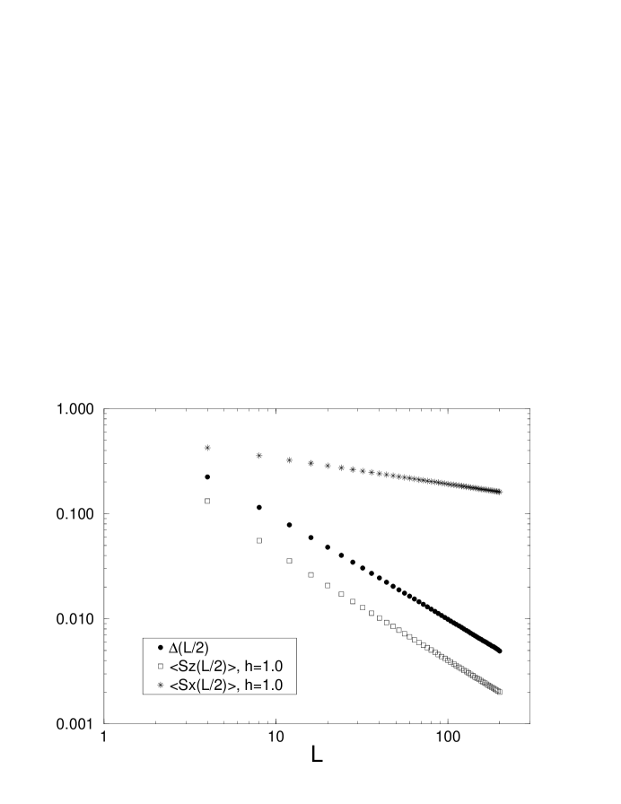
FIG. 4.: Log-log plots of induced dimerization and induced spin moments in the z-direction and x-direction (with the edge magnetic field applied in the z- and in the x-directions, respectively) at the center of the chain for the spin-$1/2$ XY model. The magnitude of the applied edge magnetic field is $h=1.0$ in both cases and the number of block states kept is $M=128$.

The exponents are obtained from the slopes of the curves shown in Fig. 4. The induced dimerization exponent for $\Delta(L/2)$ is close to $1$ ($x_{\Delta}=0.99\pm 0.01$) as expected from the relation $\nu=1/(2-x_{\Delta})$. The slope of the log-log plot of the induced spin moment in the z-direction is also close to $1$ ($x_{B}=1.01\pm 0.02$). This result is also expected since it is equivalent to the exponent for the induced density moment in the tight binding model as discussed in the previous section. In the case of the induced spin moment in the x-direction, the exponent is $0.248\pm 0.003$. This value compares well with the exact number of $1/4$ as derived in the next section.

B XXZ model

Next consider the nearest-neighbor, spin-1/2 XXZ Heisenberg antiferromagnet:

$$H=J\sum_{j=0}^{L-2}\big{[}S_{j}^{x}S_{j+1}^{x}+S_{j}^{y}S_{j+1}^{y}+\gamma S_{j}^{z}S_{j+1}^{z}\big{]}\ .$$ (29)

Anisotropy in the coupling between the z-components of the spins may be varied by changing $\gamma$. Performing the Jordan-Wigner transformation, the XY terms again yield the tight binding Hamiltonian. Low-energy excitations therefore occur near the two Fermi points at $k=\pm\pi/2a$. We may treat the non-Gaussian $\gamma$ term as a perturbation and focus on excitations around these Fermi points by defining left and right moving low-energy quasiparticles. Taking the continuum limit and keeping only the low-energy modes, the tight binding term is then effectively described by the massless fermions. The $S_{j}^{z}S_{j+1}^{z}$ term is quartic in the fermion operators. Integrating out the high-energy modes, it will renormalize the fermion velocity and also contain interaction terms.

We then implement Abelian bosonization, with UV cutoff $\alpha$. The effective Hamiltonian is a sine-Gordon model (a derivation can be found in Ref. 49):

$$H=H_{0}-\frac{y_{\phi}}{2\pi\alpha^{2}}\int dx\cos[\sqrt{8\pi}\phi(x)]$$ (30)

where

$$H_{0}=u\int dx\bigg{[}K\Pi^{2}+\frac{(\partial_{x}\phi)^{2}}{K}\bigg{]}.$$ (31)

Here $u=2Ja=2a$ is the bare Fermi velocity and the constant $K\equiv 1+y_{0}/2$ depends on the anisotropy $\gamma$. The XY limit correspond to $y_{\phi}=0$.

The long distance behavior of the staggered part of $S^{z}$ and $S^{-}$ are given in terms of the boson fields as:

$$S^{z}(x) \approx (-1)^{x/\alpha}\cos[\phi(x)/R]$$ (32)

$$S^{-}(x) \approx (-1)^{x/\alpha}e^{i2\pi R\tilde{\phi}(x)}$$ (33)

where the radius $R$ is given by[49]

$$R=\sqrt{\frac{1}{2\pi}-\frac{\cos^{-1}\gamma}{2\pi^{2}}}.$$ (34)

First consider the anisotropic case $\gamma\neq 1$. The isotropic case has logarithmic corrections to scaling that are dealt with in the next section. For $\gamma>1$ the interaction term is relevant and the system is gapped, and in the Ising universality class. Indeed, in the limit $\gamma\rightarrow\infty$ it is the Ising model. For $\gamma<1$ the interaction term is irrelevant, the system is gapless and $\Delta(L/2)$ and $\langle S^{x}(L/2)\rangle$ should exhibit power law decay, with no log corrections as there are no marginal operators. The log-log plots of Fig. 5 (a) show the induced spin moment in the x-direction at the chain center for different values of the anisotropy $\gamma$. The edge magnetic field in the x-direction is fixed, $h=1.0$. As expected, for $\gamma>1$ there is exponential decay and in the cases $\gamma<1$ the exponents $x_{B}(\gamma)$ are found by fitting the curves in Fig. 5 (a) to the form of Eq. 14. The exponents $y_{B}$ are set equal to zero, the higher order corrections are included and give very small deviations from a simple linear fit. In Fig. 5 (b) the exponents $x_{B}(\gamma)$ are compared to the exact value $x_{B}(\gamma)=\pi R^{2}(\gamma)$ obtained by Affleck[50]. Agreement is found at the percent level. Affleck derived the exponent as follows. The edge magnetic field in the x-direction applied at $j=0$ corresponds to a term

$$H_{B}=-hS^{x}(0)=-{\rm constant}\times h\cos[\sqrt{2\pi}\tilde{\phi}(0)]$$ (35)

in the Hamiltonian. For sufficiently large $h$ the energy is minimized by setting

$$\tilde{\phi}(0)=0\Longrightarrow\phi_{R}(0)=\phi_{L}(0)\ .$$ (36)

Regarding $\phi_{R}$ as an analytic continuation of $\phi_{L}$, we may identify

$$\phi_{R}(x)=\phi_{L}(-x)\ .$$ (37)

Using this boundary condition, the induced spin moment is given by

$$\langle S^{x}(j)\rangle\approx(-1)^{j/\alpha}\langle e^{i2\pi R\phi_{L}(j)}e^{-i2\pi R\phi_{L}(-j)}\rangle\approx\frac{(-1)^{j/\alpha}}{(2j)^{\pi R^{2}(\gamma)}}\ .$$ (38)

For the XY model ($\gamma=0$), the induced spin moment in the x-direction therefore decays with exponent $\pi R^{2}(0)=1/4$.

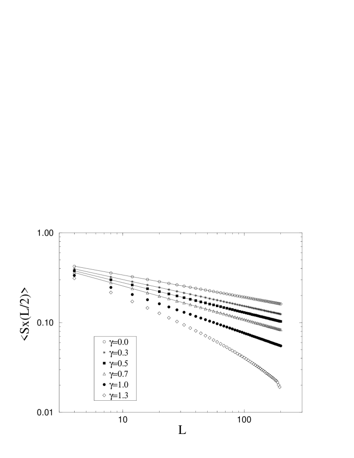
FIG. 5.: Spin-$1/2$ XXZ Heisenberg antiferromagnetic chain. (a) DMRG results ($M=128$ and $h=1.0$) for the induced spin moment in the x-direction at center of chain for different values of anisotropy $\gamma$, showing power law decay for $\gamma\leq 1$ and exponential decay for $\gamma>1$ and (b) corresponding exponent $x_{B}(\gamma)$ for $\gamma<1$. The solid line is the exact value $\pi R^{2}(\gamma)$. The exponents are obtained by fitting the curves in (a) to the form of Eq. 14 with $y_{B}=0$ since there are no logarithmic corrections away from the isotropic point.

A log-log plot of the induced dimerization at the center of the chain for various values of the anisotropy $\gamma$ is shown in Fig. 6 (a). The free boundary condition at the chain ends corresponds to setting:

$$\vec{S}_{0}=\vec{S}_{L+1}=0\ .$$ (39)

This condition translates to $\phi_{R}(x)=-\phi_{L}(-x)+\pi R$ in terms of the boson fields[51] which yields:

$$\Delta(j)~{}\approx~{}(-1)^{j/\alpha}\langle\cos[\phi(j)/R]\rangle~{}\approx~{}\frac{(-1)^{j/\alpha}}{(2j)^{1/4\pi R^{2}(\gamma)}}.$$ (40)

In Fig. 6 (b) the exponents obtained from the slopes of the curves in Fig. 6 (a) are plotted against the exact values $x_{\Delta}=1/4\pi R^{2}(\gamma)$. Again agreement is found at the percent level.

FIG. 6.: Spin-$1/2$ XXZ Heisenberg antiferromagnetic chain. (a) DMRG results ($M=128$) for the induced dimerization at center of chain for different values of anisotropy $\gamma$ and (b) corresponding exponent $x_{\Delta}(\gamma)$, obtained by fitting to Eq. 14 with $y_{\Delta}=0$. The solid line is the exact value $1/4\pi R^{2}(\gamma)$.

Another quantity of interest is the sum, instead of the difference, of the spin-spin correlation function on adjacent bonds near the center of the chain:

$$\epsilon(L/2)~{}\equiv~{}\frac{1}{2}~{}\big{(}~{}\langle\vec{S}_{L/2}\cdot\vec{S}_{L/2+1}\rangle+\langle\vec{S}_{L/2-1}\vec{S}_{L/2}\rangle~{}\big{)}~{},$$ (41)

which at $\gamma=1$ equals the energy density per bond and therefore does not vanish in the thermodynamic limit. Fig. 7 is a plot of $\epsilon(L/2)$ as a function of the system size $L$ at the isotropic point $\gamma=1$.

FIG. 7.: Sum of the two central bonds for the spin-$1/2$ XXZ Heisenberg antiferromagnetic chain at the isotropic point $\gamma=1$. The block size is $M=256$.

As expected, this quantity approaches a constant value $\epsilon(\infty)$ in the thermodynamic limit. After subtracting the extrapolated value at $L\rightarrow\infty$, $\epsilon(L/2)$ too exhibits power law decay of the form of Eq. 14. The constant $\epsilon(\infty)$ can be found by an iteration process. Starting with an initial value for $\epsilon(\infty)$ obtained from a rough extrapolation of the curve in Fig. 7, we fit the subtracted value $\epsilon(L/2)-\epsilon(\infty)$ to a power-law form. The extrapolated value $\epsilon(\infty)$ is then adjusted slightly until an optimal fit to a pure power law is attained. The extrapolated value found this way is $\epsilon(\infty)=-0.443148$ and Fig. 8 shows the power law behavior of the subtracted quantity.

FIG. 8.: Log-log plot of $\epsilon(L/2)$ after subtracting the extrapolated value $\epsilon(\infty)=-0.443148$. The fit is to a straight line of slope $2.14$.

We obtain an exponent of $2.1\pm 0.1$ in the scaling of $\epsilon(L/2)-\epsilon(\infty)$. This is as expected from the linear dispersion relation of Heisenberg antiferromagnets: in a Lorentz-invariant theory the energy density operator has dimension 2.

The DMRG result for the energy per bond is extremely accurate and can be compared with the exact value obtained from the Bethe ansatz solution[52] of $~{}\epsilon=1/4-\ln 2=-0.44314718$. It is crucial to note that the open boundary conditions induce staggering in the strength of the bonds along the chain. To eliminate this effect, the energy per bond must be calculated as the average of the bond energy from two consecutive bonds at the center of the chain. Suggestions that infinite-size DMRG results for the center region of the chain are not very accurate[53] appear to have failed to take this effect into account. We have also checked our results at different anisotropies. For the XY case ($\gamma=0.0$), we obtain $\epsilon(\infty)=-0.318310$ extrapolating from chains up to $L=200$ and $M=128$ and the exact result[52] is $-1/\pi=-0.3183099$.

C Logarithmic Corrections to Scaling

In the isotropic XXX limit, the interaction $\cos[\sqrt{8\pi}\phi(x)]$ in the low-energy effective Hamiltonian Eq. 30 becomes marginal and can generate multiplicative logarithmic corrections to scaling. In this section we calculate its effect on the scaling of the induced spin moment $\langle S^{x}(L/2)\rangle$ when an edge magnetic field $H_{B}$ in the x-direction is applied. Cancellations occur and in this case there are no multiplicative $\ln(L)$ corrections. As a practical matter, the cancellation of the logarithmic corrections means that numerical calculations of the exponent $x_{B}$ are particularly precise. We note that finite-size scaling of the spin-spin correlation function has been previously calculated for a spin-$1/2$ chain with periodic boundary conditions[54, 55].

The coupling constants in the sine-Gordon Hamiltonian (Eq. 30) renormalize under a change of the ultraviolet cutoff $\alpha\rightarrow\alpha e^{l}$ according to the renormalization group equations[56]:

$$\frac{dy_{0}}{dl} = -y_{\phi}^{2}(l),$$ (42)

$$\frac{dy_{\phi}}{dl} = -y_{\phi}(l)y_{0}(l).$$ (43)

As noted in the previous section, a large edge magnetic field applied at $x=0$ in the x-direction enforces the boundary condition $\phi_{R}(x)=\phi_{L}(-x)$ (Eq. 37). Thus

$$\langle S^{x}(x)\rangle\sim(-1)^{x/a}\langle\cos[\sqrt{2\pi}\tilde{\phi}(x)]\rangle\sim\langle e^{i\sqrt{2\pi}\phi_{L}(x)}e^{-i\sqrt{2\pi}\phi_{L}(-x)}\rangle.$$ (44)

For the free theory, which corresponds to the XY model $y_{\phi}=0$, the induced spin moment is simply

$$\langle S^{x}(x)\rangle_{0}\sim\exp\big{[}-KU_{L}(2x)\big{]}$$ (45)

where

$$U_{L}(x)=\frac{1}{2}\ln(\frac{\alpha+ix}{\alpha}).$$ (46)

But in the general XXZ case we ascertain the effect of the marginal operator by following a procedure similar to one developed by Giamarchi and Schulz[56] who calculated correlation functions for finite periodic chains. We first define the function:

$$F(x)\equiv e^{KU_{L}(2x)}\langle S^{x}(x)\rangle\ .$$ (47)

At the XY point $y_{\phi}=0$ clearly $F(x)=1$. For small $x$, an expansion of $F$ in powers of $y_{\phi}$ converges, and for sufficiently small coupling $y_{\phi}$, $F(x)\sim 1$. Upon rescaling, the function $F(x)$ also depends on the new length scale and on the rescaled coupling constants $y_{0}(l)$ and $y_{\phi}(l)$. By an argument similar to the one employed by Kosterlitz[57], the effect of rescaling $\alpha\rightarrow e^{l}~{}\alpha$ is:

$$F(x,\alpha e^{l},y(l))=I(dl,y(l))F(x,\alpha e^{l+dl},y(l+dl))\ ,$$ (48)

where $y(l)$ denotes all the couplings as function of the scaling parameter $l$. The rescaled short distance cutoff is then $\alpha(l)=e^{l}~{}\alpha$, where $\alpha$ is the initial cutoff. Rescaling can be repeated until $\alpha(l)\sim x$, at which point we have:

$$F(x,x,y(\ln(x/\alpha)))=O(1)\ .$$ (49)

The contributions to the function $F$ from repeated rescalings, until $\alpha(l)$ reaches $x$, can be written explicitly as:

$$F(x,\alpha,y(\alpha))=\prod_{l=0}^{l=\ln(x/\alpha)}I(dl,y(l))=\exp\bigg{\{}\int_{0}^{\ln(x/\alpha}\ln\big{[}I(dl,y(l))\big{]}dl\bigg{\}}\ .$$ (50)

We proceed to calculate the function $I$. First we expand $\langle S^{x}(x)\rangle$ in powers of $y_{\phi}$, writing it in terms of averages with respect to the free Hamiltonian,

$$\langle S^{x}(x)\rangle \sim e^{-KU_{L}(2x)}+\frac{y_{\phi}}{2\pi\alpha^{2}}\int d^{2}x^{\prime}\langle S^{x}(x)\cos[\sqrt{8\pi}\phi(x^{\prime})]\rangle_{0}+$$ (52)

$$\frac{1}{2}\big{(}\frac{y_{\phi}}{2\pi\alpha^{2}}\big{)}^{2}\int d^{2}x_{1}\int d^{2}x_{2}\langle S^{x}(x)\cos[\sqrt{8\pi}\phi(x_{1})]\cos[\sqrt{8\pi}\phi(x_{2})]\rangle_{0}+\ldots$$

The averages are given by

$$\langle S^{x}(x)\cos[\sqrt{8\pi}\phi(x^{\prime})]\rangle_{0}=0$$ (53)

and

$$\langle S^{x}(x)\cos[\sqrt{8\pi}\phi(x_{1})] \cos[\sqrt{8\pi}\phi(x_{2})]\rangle_{0}\sim$$ (55)

$$\frac{1}{2}\exp\big{[}-KU_{L}(2x)+4KU_{L}(2x_{1})+4KU_{L}(2x_{2})-4KU(x_{1}+x_{2})-4KU(x_{1}-x_{2})\big{]}$$

The $O(y_{\phi}^{2})$ term can be simplified by assuming that the main contribution comes from configurations where $x_{1}$ and $x_{2}$ are very close to each other[58, 56]. Introducing new integration variables

$$r \equiv x_{1}-x_{2}$$ (56)

$$R \equiv \frac{x_{1}+x_{2}}{2}$$ (57)

and expanding $U_{L}$ in powers of $r$, which is assumed to be small,

$$U_{L}(2x_{1})=U_{L}(2R+r)=U_{L}(2R)+r~{}\partial_{R}~{}U_{L}(2R)+\ldots\ ,$$ (58)

$$U_{L}(2x_{2})=U_{L}(2R-r)=U_{L}(2R)-r~{}\partial_{R}~{}U_{L}(2R)+\ldots\ ,$$ (59)

we obtain the average

$$\langle S^{x}(x)\cos[\sqrt{8\pi}\phi(x_{1})]\cos[\sqrt{8\pi}\phi(x_{2})]\rangle_{0}\sim\frac{1}{2}\exp\left[-KU_{L}(2x)-4KU(r)\right]\ .$$ (60)

The dependence on $R$ cancels out. The expansion Eq. 52 becomes

$$\langle S^{x}(x)\rangle \sim e^{-KU_{L}(2x)}\bigg{[}1+\frac{y_{\phi}^{2}\Omega}{4\alpha^{2}}\int_{\alpha}dre^{-4KU(r)}\bigg{]}\ ,$$ (61)

where $\Omega\equiv\int dR$ is a measure of the linear size of the system. Next consider the effect of rescaling $\alpha^{\prime}=\alpha e^{dl}$, where $dl$ is infinitesimal. Using

$$\int_{\alpha}^{\infty}dx=\int_{\alpha}^{\alpha^{\prime}}dx+\int_{\alpha^{\prime}}^{\infty}dx\ \ ,$$ (62)

we obtain:

$$\langle S^{x}(x)\rangle\sim e^{-KU_{L}(2x)}\bigg{[}1+\frac{y_{\phi}^{2}}{4\alpha^{2}}dl+\frac{y_{\phi}^{\prime 2}}{4\alpha^{\prime 2}}\int_{\alpha^{\prime}}dre^{-4KU(r)}\bigg{]}$$ (63)

Matching this result with Eq. 48, we find:

$$I(dl,y_{0}(l),y_{\phi}(l))\sim\exp\bigg{[}\frac{y_{\phi}^{2}(l)}{4\alpha^{2}}dl\bigg{]}\ ,$$ (64)

hence from Eq. 50 and Eq. 47, we have

$$\langle S^{x}(x)\rangle\sim\exp\bigg{\{}-KU_{L}(2x)+\int_{0}^{\ln(x/\alpha)}\frac{y_{\phi}^{2}(l)}{4\alpha^{2}}dl\bigg{\}}\ .$$ (65)

Using the RG equations (Eq. 43), the solution at large $l$ is $y_{\phi}(l)\sim 1/l$ and

$$\langle S^{x}(x)\rangle\sim\bigg{(}\frac{x}{\alpha}\bigg{)}^{-1/2}\exp\bigg{\{}\int_{0}^{\ln(x/\alpha)}dl\big{[}~{}O(\frac{1}{l^{2}})~{}\big{]}\bigg{\}}\ .$$ (66)

There are no multiplicative $\ln(x)$ corrections, as these would require terms of order $O(1/l)$ in the integrand inside the exponential in Eq. 66. In our calculation, $O(1/l)$ terms do not appear, only $O(1/l^{2})$ and higher-order terms. As a check, we can repeat the same procedure for $\langle S^{z}(x)\rangle$, with the edge field now oriented in the z-direction. Of course this should give the same result since the system is isotropic, but as the Jordan-Wigner transformation picks the z-direction as the spin quantization axis, the equivalence is not obvious, and the check is non-trivial. Again, explicit calculation shows that $O(1/l)$ terms do not arise. This result is in reasonable agreement with our numerical results. Fitting the DMRG data (see Fig. 9) to the form Eq. 14, we obtain $x_{B}=0.485\pm 0.01$ with a small non-zero value for the log exponent $y_{B}=0.06\pm 0.01$. By contrast, in the case of the induced dimerization we obtain $x_{\Delta}=0.57\pm 0.01$ and $y_{\Delta}=0.10\pm 0.05$. The error was estimated from deviations obtained by fitting the $M=128$ data over different ranges of L ($4\leq L\leq 600$) and by comparison with $M=64$ data ($4\leq L\leq 300$). Results are systematically improved by increasing the value of $M$.

FIG. 9.: Log-log plot of the induced spin moment ($h=1.0$) and induced dimerization at center of chain for the isotropic $S=1/2$ Heisenberg antiferromagnet. Data obtained using block Hilbert space size of $M=128$ and $M=64$ are plotted for comparison. Note the slight curvature in $\Delta(L/2)$ which signals the existence of multiplicative logarithmic corrections to scaling. The log is absent in the plot of $\langle S^{x}(L/2)\rangle$. The discrepancy in the induced dimerization at large chain length is due to the truncation of the block Hilbert space.

Finite-size scaling behavior for the XXX model with open boundary conditions[35] and periodic boundary conditions[34] were obtained from DMRG calculations of ground state energies and correlation functions $\langle S^{z}(x)S^{z}(x+r)\rangle$ for different system sizes and separations $r$. In our approach, critical exponents are extracted from expectation values at the center of the chain only. The chain size is increased via the infinite-size DMRG method. It is also advantageous to extract power law exponents when there are no logarithmic corrections.

D Conformal Anomaly

Finally, we may calculate the value of the conformal anomaly, $c$. We note that the central charge of the RSOS model[60] and of the spin-$3/2$ Heisenberg chain[34], which is in the same universality class as the spin-$1/2$ chain, have previously been obtained using the DMRG. The conformal anomaly can be extracted by finding the coefficient of the $1/L$ finite-size correction to the free energy, equivalent at zero temperature to the ground state energy. We fit the ground state energy $E_{0}(L)$ to the following form:

$$E_{0}(L)=AL+B+C/L+\ldots$$ (67)

The extensive contribution, proportional to $A$, and the constant term $B$ are non-universal. At the isotropic point $\gamma=1$ our results for the case of blocksize $M=128$ and for chain lengths in the range $30\leq L\leq 100$ yield $C\approx-0.323$. To relate this coefficient to the conformal anomaly we must normalize it by dividing by the speed of low-lying excitations, $v$. The speed can be obtained by extrapolation to the thermodynamic limit of the gap to the lowest-lying excitation multiplied by the chain length:

$$v=\lim_{L\rightarrow\infty}~{}{{{\rm Gap}(L)\times L}\over{\pi}}\ .$$ (68)

We find $v=2.44$. Now for open boundary conditions[59],

$$c={{-24C}\over{\pi v}}\approx 1.01\ .$$ (69)

This compares well with the value of $c=1$ appropriate for a single boson or the pair of left and right moving fermions.

V Spin-$1$ chain

As a final example we apply the DMRG / finite-size scaling method to the isotropic spin-$1$ antiferromagnetic chain. This problem is more challenging numerically as the on-site Hilbert space now has dimension $D=3$ instead of $D=2$. The most general nearest-neighbor Hamiltonian for the spin-$1$ chain includes the possibility of a biquadratic spin-spin interaction term:

$$H=\sum_{j=0}^{L-2}\big{[}\cos\theta~{}\vec{S}_{j}\cdot\vec{S}_{j+1}+\sin\theta~{}(\vec{S}_{j}\cdot\vec{S}_{j+1})^{2}\big{]}$$ (70)

The phase diagram can be represented on a circle parameterized by $\theta$ as depicted in Fig. 10.

FIG. 10.: Phase diagram for isotropic, nearest-neighbor, S=1 chain, parameterized by the angle $\theta$. A critical point at $\theta=-\pi/4$ separates the Haldane and dimerized phases, both of which are gapped. At $\theta=\tan^{-1}(1/3)$, the ground state is a valence bond solid (VBS), as depicted in the schematic. Each oval represents an atom; the two black dots inside the oval are two electrons symmetrized into a triplet $S=1$ spin state. Rectangles represent singlet bonds which encompass two electrons on adjacent sites. In the dimerized phase, singlet correlations are instead enhanced on alternating dimers.

Generically there is a gap to excitations in the antiferromagnetic region of the phase diagram, in accord with the Haldane conjecture[62]. The point $\theta=0$ corresponds to the usual pure bilinear Heisenberg antiferromagnet. At the point $\tan\theta=1/3$ the Hamiltonian can be written as a sum of positive-definite projection operators, and the exact ground state is the AKLT valence bond solid (VBS)[61]. Negative $\sin\theta$ favors dimerization, as the energy is minimized by concentrating singlet correlations on isolated dimers. The dimerized phase also is gapped: a dimer must be broken to generate a spin excitation. The point that separates the dimerized and Haldane phases lies at $\theta=-\pi/4$ and can be solved exactly by the Bethe ansatz[63, 64]. The chain is quantum critical at this integrable point. The ground state is non-degenerate here as well as in the dimerized and Haldane phases.

DMRG calculations clearly delineate the two massive phases and the critical point separating them, even for relatively small block Hilbert sizes $M$. In Figs. 11 and 12, the blocksize $M=81$ for the massive phases. Thus the results are numerically exact up only to chain lengths $L=10$. For chain lengths $L>10$ the Hilbert space is truncated via the DMRG algorithm. To increase accuracy, results at the critical point were obtained with a larger Hilbert size for the blocks, $M=256$.

FIG. 11.: Induced spin moment at center of a spin-$1$ chain for different values of $\theta$. Here $h=1$. Note the power law decay at the critical point ($\theta=-\pi/4$). Exponential decay occurs at the AKLT valence bond solid point [$\theta=\arctan(1/3)=0.321751$] within the Haldane phase and in the dimerized phase at $\theta=-\pi/2$. Results at the critical point were obtained with $M=256$, while $M=81$ for the other two cases.

FIG. 12.: Induced dimerization at center of a spin-$1$ chain. Again we set $M=256$ at the critical point and $M=81$ for the two massive phases. There is power law decay at the critical point ($\theta=-\pi/4$) and exponential decay at the AKLT point. As expected the dimerization approaches a non-zero constant in the dimerized phase ($\theta=-\pi/2$).

The induced spin moment at the center of the chain decays exponentially in both the Haldane and the dimerized phases, as expected. The induced dimerization at the chain center also decays exponentially in the Haldane phase, but approaches a non-zero constant in the dimerized phase as it must. Power law decay in both observables occurs at the critical point. Fitting the $M=256$ data shown in Fig. 12 at the critical point $\theta=-\pi/4$ we obtain dimerization exponents $x_{\Delta}=0.37\pm 0.01$ and $y_{\Delta}=0.3\pm 0.05$, reflecting the apparent presence of a marginal interaction and consequent multiplicative logarithmic corrections to scaling. Likewise, for a field of $h=1.0$ applied to the chain ends, the exponents for the spin operator are $x_{B}=0.34\pm 0.01$ and $y_{B}=0.23\pm 0.05$. The values of the exponents compare to the exact values[65, 66] $x_{\Delta}=3/8\approx 0.375$ and $x_{B}=3/8$. To the best of our knowledge there are no analytic results at the integrable point $\theta=-\pi/4$ (which corresponds to a $k=2$ SU(2) WZW model) on the size of the logarithmic corrections $y_{\Delta}$ and $y_{B}$, at least for open boundary conditions.

Finally, we may repeat the analysis of the conformal anomaly described above in subsection IV D for the case of the spin-1 chain at its critical point. For $M=256$ and fitting over chain lengths $10\leq L\leq 26$ we find that the speed of excitations is $v=3.69$, $C=0.508$, and hence $c=1.05$. This value is close to its exact value of 1, demonstrating that the conformal anomaly can be reliably extracted even from relatively short chains.

VI Conclusion

We have presented a simple method for studying critical behavior of quantum spin chains. Accurate critical exponents can be extracted. For small on-site Hilbert space sizes ($D=2$ for the spin-$1/2$ chain and $D=3$ for spin-$1$ chains) the method does not require supercomputers. Results can be systematically improved by increasing the size of $M$, the dimension of the Hilbert space retained in the blocks, up to limits set by machine memory and speed. The DMRG method works best for massive, non-critical, systems, but it is also quite accurate even at critical points. Critical exponents can be calculated at percent level accuracy. We showed that the leading multiplicative logarithmic correction to the scaling of the induced spin moment cancels out in the case of the isotropic spin-$1/2$ Heisenberg antiferromagnet. Thus accurate exponents can sometimes be found numerically despite the presence of marginal interactions.

Use of the “finite-size” DMRG algorithm might improve the method, but good results were obtained with the relatively simpler “infinite-size” DMRG algorithm. The reason for this is that the finite-size scaling method employed here focuses on the scaling of observables near the center of the chain only, where the “infinite-size” algorithm is particularly accurate. The method can be used to study new systems. For example, several non-interacting but disordered electron systems, like the integer and spin quantum Hall transitions, can be described by supersymmetric Hamiltonians[67, 68]. In a paper which follows[1], we employ the combined DMRG/finite-size method in combination with analytic calculations to understand the behavior of these supersymmetric spin chains.

Acknowledgments We thank I. Affleck, M. P. A. Fisher, V. Gurarie, J. Kondev, M. Kosterlitz, A. Ludwig and T. Senthil for useful discussions. This work was supported in part by the NSF under Grants Nos. DMR-9357613, DMR-9712391. Computations were carried out in double-precision C++ on Cray PVP machines at the Theoretical Physics Computing Facility at Brown University.

REFERENCES

- [1] S.-W. Tsai and J. B. Marston, Density-matrix renormalization-group analysis of quantum critical points. II. Supersymmetric spin chains, unpublished.
- [2] S. R. White, Phys. Rev. Lett. 69, 2863 (1992); Phys. Rev. B 48, 10345 (1993).
- [3] I. Peschel, X. Wang, M. Kaulke and K. Hallberg, eds., “Density-matrix renormalization — a new numerical method in physics” (Springer-Verlag, Berlin, Heidelberg, 1999).
- [4] S. R. White and D. A. Huse, Phys. Rev. B 48, 3844 (1993).
- [5] E. S. Sørensen and I. Affleck, Phys. Rev. Lett. 71, 1633 (1993), Phys. Rev. B 49, 13235 (1994).
- [6] E. S. Sørensen and I. Affleck, Phys. Rev. B 49, 15771 (1994).
- [7] T.-K. Ng, S. Qin and Z.-B. Su, Phys. Rev. B 54, 9854 (1996).
- [8] R. J. Bursill, T. Xiang and G. A. Gehring, J. Phys. A - Math. Gen. 28, 2109 (1995).
- [9] G. Fáth and J. Sólyom, Phys. Rev. B 51, 3620 (1995).
- [10] U. Schollwöck and T. Jolicoeur, Europhys. Lett. 30, 493 (1995), U. Schollwöck, O. Golinelli and T. Jolicoeur, Phys. Rev. B 54, 4038 (1996).
- [11] X. Wang, S. Qin and L. Yu, Phys. Rev. B 60, 14529 (1999).
- [12] Y. Kato and A. Tanaka, J. Phys. Soc. Jpn. 63, 1277 (1994).
- [13] R. Bursill, G. A. Gehring, D. J. J. Farnell, J. B. Parkinson, T. Xiang and C. Zeng, J. Phys. C 7, 8605 (1995).
- [14] R. Chitra, S. Pati, H. R. Krishnamurthy, D. Sen and S. Ramasesha, Phys. Rev. B 52, 6581 (1995), S. Pati, R. Chitra, D. Sen, H. R. Krishnamurthy and S. Ramasesha, Europhys. Lett. 33, 707 (1996), S. Pati, R. Chitra, D. Sen, S. Ramasesha and H. R. Krishnamurthy, J. Phys. - Cond. Mat. 9, 219 (1997).
- [15] A. Kolezhuk, R. Roth and U. Schollwöck, Phys. Rev. B 55, 8928 (1997).
- [16] S. Watanabe and H. Yokoyama, J. Phys. Soc. Jpn. 68, 2073 (1999).
- [17] R. Roth and U. Schollwöck, Phys. Rev. B 58, 9264 (1998).
- [18] S. Qin, T.-K. Ng and Z.-B. Su, Phys. Rev. B 52, 12844 (1995).
- [19] E. Polizzi, F. Mila and E. S. Sorensen, Phys. Rev. B 58, 2407 (1998).
- [20] Ö. Legeza and J. Sólyom, Phys. Rev. B 59, 3606 (1999).
- [21] A. Juozapavicius, S. Caprara and A. Rosegren, Phys. Rev. B 60, 14771 (1999).
- [22] K. Hida, J. Phys. Soc. Jpn. 65, 895 (1996), J. Phys. Soc. Jpn. 66, 330 (1997), J. Phys. Soc. Jpn. 66, 3237 (1997), Phys. Rev. Lett. 83, 3297 (1999).
- [23] F. Schönfeld, G. Bouzerar, G. S. Uhrig and E. Müller-Hartmann, Eur. Phys. J. B 5, 521 (1998).
- [24] K. Hida, J. Phys. Soc. Jpn. 68, 3177 (1999).
- [25] S. K. Pati, S. Ramasesha and D. Sen, Phys. Rev. B 55, 8894 (1997), J. Phys. - Condens. Mat. 9, 8707 (1997).
- [26] L. Campos Venuti, E. Ercolessi, G. Morandi, P. Pieri and M. Roncaglia, “Spin chains in an external magnetic field. Closure of the Haldane gap and effective field theories.”, cond-mat/9908044.
- [27] J. Lou, X. Dai, S. Qin, Z. Su and L. Yu, Phys. Rev. B 60, 52 (1999).
- [28] X. Wang and S. Mallwitz, Phys. Rev. B 53, R492 (1996).
- [29] E. S. Sørensen and I. Affleck, Phys. Rev. B 51, 16115 (1995).
- [30] L. G. Caron and S. Moukouri, Phys. Rev. Lett. 76, 4050 (1996).
- [31] R. J. Bursill, R. H. McKenzie and C. J. Hamer, Phys. Rev. Lett. 83, 408 (1999).
- [32] A. Drzewiński and J. M. J. van Leeuwen, Phys. Rev. B 49, 403 (1994), A. Drzewiński and R. Dekeyser, Phys. Rev. B 51, 15218 (1995).
- [33] R. J. Bursill and F. Gode, J. Phys. - Condens. Mat. 7, 9765 (1995).
- [34] K. A. Hallberg, P. Horsch and G. Martínez, Phys. Rev. B 52, R719 (1995); K. Hallberg, X. Q. G. Wang, P. Horsch and A. Moreo, Phys. Rev. Lett. 76, 4955 (1996).
- [35] T. Hikihara and A. Furusaki, Phys. Rev. B 58, R583 (1998).
- [36] J. Kondev and J. B. Marston, Nucl. Phys. B 497, 639 (1997).
- [37] E. Carlon, M. Henkel and U. Schollwöck, Eur. Phys. J. B 12, 99 (1999).
- [38] E. Carlon and F. Iglói, Phys. Rev. B 57, 7877 (1998), E. Carlon, C. Chatelain and B. Berche, Phys. Rev. B 60, 12974 (1999).
- [39] M. Kaulke and I. Peschel, Eur. Phys. J. B 5,727 (1998).
- [40] T. Senthil, J. B. Marston, and M. P. A Fisher, Phys. Rev. B 60, 4245 (1999).
- [41] I. Gruzberg, A. Ludwig, and N. Read, Phys. Rev. Lett. 82, 4524 (1999).
- [42] T. Nishino, J. Phys. Soc. Jpn. 64, 3598 (1995).
- [43] E. Carlon and A. Drzewiński, Phys. Rev. Lett. 79, 1591 (1997).
- [44] Y. Honda and T. Horiguchi, Phys. Rev. E 56, 3920 (1997).
- [45] M. Andersson, M. Boman and S Östlund, Phys. Rev. B 59, 10493 (1999).
- [46] M. E. Fisher and P.-G. de Gennes, C. R. Acad. Sc. Paris B 287, 207 (1978).
- [47] F. Igloi and H. Rieger, Phys. Rev. Lett. 78, 2473 (1997).
- [48] P. Jordan and E. Wigner, Z. Phys. 47, 631 (1928).
- [49] I. Affleck in Fields, Strings and Critical Phenomena, E. Brezin and J. Zinn-Justin eds. (North-Holland, Amsterdam 1990).
- [50] I. Affleck, J. Phys. A 31, 2761 (1998).
- [51] S. Eggert and I. Affleck, Phys. Rev. B 46, 10,866 (1992).
- [52] R. Baxter, Ann. of Phys. (NY) 70, 193 (1972), Ann. of Phys. (NY) 70, 323 (1972).
- [53] H. Tasaki, T. Hikihara and T. Nishino, J. Phys. Soc. Jpn. 68, 1537 (1999).
- [54] V. Barzykin and I. Affleck, J. Phys. A 32, 867 (1999).
- [55] I. Affleck, J. Phys. A 31, 4573 (1998).
- [56] T. Giamarchi and H. J. Schulz, Phys. Rev. B 39, 4620 (1989).
- [57] J. M. Kosterlitz, J. Phys. C 7, 1046 (1974).
- [58] D. R. Nelson, Phys. Rev. B 18, 2318 (1978).
- [59] J. Cardy in Fields, Strings and Critical Phenomena, p. 202 – 203, E. Brezin and J. Zinn-Justin eds. (North-Holland, Amsterdam 1990).
- [60] G. Sierra and T. Nishino, Nucl. Phys. B 495, 505 (1997).
- [61] I. Affleck, T. Kennedy, E. H. Lieb and H. Tasaki, Phys. Rev. Lett. 59, 799 (1987).
- [62] F. D. M. Haldane, Phys. Rev. Lett. 50, 1153 (1983); Phys. Lett. A 93, 464 (1983).
- [63] L. A. Takhtajan, Phys. Lett. A 87, 479 (1982).
- [64] H. M. Babudjian, Phys. Lett. A 90, 479 (1982); Nucl. Phys. B 215, 317 (1983).
- [65] I. Affleck, D. Gepner, H. J. Schultz and T. Ziman, J. Phys. A 22, 511 (1989).
- [66] I. Affleck, Phys. Rev. Lett. 62, 839 (1989).
- [67] J. B. Marston and Shan-Wen Tsai, Phys. Rev. Lett. 82, 4906 (1999).
- [68] Shan-Wen Tsai and J. B. Marston, Annalen der Physik, 8 Special Issue, 261 (1999).