Generalization of ${\bf k\cdot p}$ theory for periodic perturbations

Abstract

We extend standard ${\bf k\cdot p}$ theory to take into account periodic perturbations which are rapidly oscillating with a wavelength of a few lattice constants. Our general formalism allows us to explicitly consider the Bragg reflections due to the perturbation-induced periodicity. As an example we calculate the effective masses in the lowest two conduction bands of spontaneously ordered GaInP₂ as a function of the degree of ordering. Comparison of our results for the lowest conduction band to available experimental data and to first principle calculations shows good agreement.

I Introduction

For many years ${\bf k\cdot p}$ theory[2, 3] has been very successful in describing a wide variety of crystal band structures, an important merit being that it allows one to derive simple, analytical formulas which capture the essential physics. In the presence of perturbing potentials it becomes the envelope function approximation (EFA),[4] which has been successfully applied to such different problems as impurities[5] and semiconductor heterostructures.[6] However, the EFA requires the perturbation potential $V_{1}({\bf r})$ to be slowly varying on the length scale of the lattice constant, i.e., the nonzero Fourier components of the potential $V_{1}({\bf r})$ must be restricted to wave vectors which are small compared to the dimensions of the Brillouin zone. Some authors[7, 8] reported problems with the EFA for systems where this requirement is not fulfilled, notably in artificial and natural short-period superlattices such as spontaneously ordered GaInP₂. These superlattices can be viewed as systems with a periodic perturbation, where the smallest Fourier components of the perturbation are comparable to the dimensions of the Brillouin zone of the unperturbed problem. These Fourier components result in interactions between states with very different wave vectors, which are crucial for the properties of these short-period superlattices. However, the interactions cannot be accurately described within standard ${\bf k\cdot p}$ theory.[4] In this paper we present a general method which allows us to treat perturbing potentials which are rapidly oscillating but commensurate to the periodicity of the potential of the unperturbed problem. To illustrate the method, we apply it to the natural superlattice of spontaneously ordered GaInP₂.

The Ga_xIn_1-xP alloy for $x\approx 0.51$ can be lattice matched grown on a GaAs$(001)$ substrate. Under proper growth conditions, long-range order of the CuPt type is observed.[9, 10] This type of ordering is characterized by $\langle 111\rangle$ layers alternatingly rich in Ga or In. In the ordered material the symmetry of the lattice is reduced from $T_{d}$ to $C_{3v}$, and the Brillouin zone becomes smaller than the zinc-blende Brillouin zone, which leads to a backfolding of states. The change in the crystal potential induced through the ordering is a short-period potential that mixes electronic states of an “averaged” zinc-blende structure. In particular, the interactions between $\Gamma$ and L states lead to energy shifts of the band-edge states in the ordered alloy, which cause band-gap reduction and valence-band splitting. These effects have been investigated theoretically[11, 12] and experimentally.[9, 13, 14] In addition to the changes in the energies, the effective masses are also altered. Raikh and Tsiper[15] calculated the conduction-band effective mass of ordered GaInP₂ using a two-band model, which accounts only for the mixing of conduction-band $\Gamma$ and L states. They found that the effective mass parallel to the ordering direction $m_{\parallel}$ and the effective mass perpendicular to the ordering direction $m_{\perp}$ increase with increasing ordering, and that $m_{\parallel}$ is larger than $m_{\perp}$. This model, however, does not take into account the change of the interaction between conduction- and valence-band states due to the band-gap reduction and valence-band splitting. These changes were investigated by Zhang and Mascarenhas[16] with an eight-band ${\bf k\cdot p}$ model, which included zinc-blende $\Gamma$ states from both the conduction and valence band. They find $m_{\parallel}$ and $m_{\perp}$ to decrease with increasing ordering, with $m_{\parallel}$ being larger than $m_{\perp}$. A third investigation was done by Franceschetti, Wei, and Zunger,[8] who performed first-principle calculations using the local-density approximation. They find $m_{\parallel}$ to increase, whereas $m_{\perp}$ decreases with increasing ordering. This result agrees qualitatively with the only measurment that investigated the anisotropy of the effective masses in ordered GaInP₂.[17] In Ref. [8] the conclusion was drawn that the conduction-band effective masses in ordered GaInP₂ depend on a “delicate balance” of $\Gamma$–L mixing and increased interaction between conduction and valence band. However, the $\Gamma$–L mixing and the increase of the interaction between conduction and valence bands have a common source in the ordering-induced $\Gamma$–L interactions. The conduction band masses in partially ordered GaInP₂ present an excellent test for our theory, which should be able to describe that “delicate balance.”

This paper is organized as follows. In Sec. II we derive a general scheme applicable to periodic perturbations within ${\bf k\cdot p}$ theory. In Sec. III we use this theory to derive a model for the conduction band of spontaneously ordered GaInP₂. The results are discussed in Sec. IV. A summary and a short outlook are presented in Sec. V.

II General Theory

We consider a system with the one-particle Hamiltonian

$$H_{0}=\frac{{\bf p}^{2}}{2m}+V_{0}({{\bf r}}),$$ (1)

where ${\bf p}$ is the momentum operator, $m$ the free-electron mass, and $V_{0}({{\bf r}})$ the periodic potential of the crystal. In the case of the GaInP₂ alloy, $V_{0}({{\bf r}})$ is an averaged potential of the disordered material. The eigenfunctions of the Hamiltonian $H_{0}$ are Bloch functions $\psi_{n{\bf k}}({{\bf r}})=e^{i{\bf k}\cdot{\bf r}}u_{n{\bf k}}({{\bf r}})$ with eigenvalues $\varepsilon_{n}({\bf k})$

$$H_{0}\psi_{n{\bf k}}=\varepsilon_{n}({\bf k})\psi_{n{\bf k}}.$$ (2)

Here ${\bf k}$ is a wave vector in the first Brillouin zone (BZ₀), which corresponds to the periodicity of $V_{0}({{\bf r}})$.

In conventional ${\bf k\cdot p}$ theory, basis functions

$$\chi^{{\bf k}_{0}}_{n{\bf k}}({\bf r})=e^{i{\bf k}\cdot{\bf r}}\psi_{n{\bf k}_{0}}({\bf r})=e^{i{\bf k}\cdot{\bf r}}e^{i{\bf k}_{0}\cdot{\bf r}}u_{n{\bf k}_{0}}({\bf r}),$$ (3)

are introduced, where ${\bf k}$ belongs to BZ₀. As shown by Luttinger and Kohn,[4] the functions $\chi^{{\bf k}_{0}}_{n{\bf k}}$ provide a complete and orthonormal basis set for any ${\bf k}_{0}$ being an element of BZ₀. Thus any eigenfunction of $H_{0}$ can be expanded in terms of $\chi^{{\bf k}_{0}}_{n{\bf k}}$

$$\phi_{n^{\prime\prime}}({\bf r})=\sum_{n^{\prime}}\int\limits_{\text{BZ{\hbox{_{0}}}}}d^{3}k^{\prime}\,c_{n^{\prime\prime}n^{\prime}}({\bf k}^{\prime})\chi^{{\bf k}_{0}}_{n^{\prime}{\bf k}^{\prime}}({{\bf r}}),$$ (4)

which yields the well-known ${\bf k\cdot p}$ equation for expansion coefficients $c_{n^{\prime\prime}n}({\bf k})$ and energy $\varepsilon_{n^{\prime\prime}}({\bf k}_{0}+{\bf k})$

$$\sum_{n^{\prime}}H^{{\bf k}_{0}}_{nn^{\prime}}({\bf k})c_{n^{\prime\prime}n^{\prime}}({\bf k})=\varepsilon_{n^{\prime\prime}}({\bf k}_{0}+{\bf k})c_{n^{\prime\prime}n}({\bf k}),$$ (5)

with

$$H^{{\bf k}_{0}}_{nn^{\prime}}({\bf k})=\left(\varepsilon_{n}({\bf k}_{0})+\frac{\hbar^{2}}{2m}k^{2}\right)\delta_{nn^{\prime}}+\frac{\hbar}{m}{\bf k}\cdot{\bf p}^{{\bf k}_{0}}_{nn^{\prime}}.$$ (6)

The momentum matrix element ${\bf p}^{{\bf k}_{0}}_{nn^{\prime}}$ is defined as

$${\bf p}^{{\bf k}_{0}}_{nn^{\prime}}={\frac{(2\pi)^{3}}{\Omega_{0}}}\int d^{3}r\,e^{-i{\bf k}_{0}{\bf\cdot r}}u_{n{\bf k}_{0}}^{\ast}{\bf p}e^{i{\bf k}_{0}{\bf\cdot r}}u_{n^{\prime}{\bf k}_{0}}.$$ (7)

Here the integration extends over the unit cell with volume $\Omega_{0}$. Equation (5) is diagonal with respect to ${\bf k}$ due to the periodicity of $V_{0}({\bf r})$, i.e., ${\bf k}$ is a good quantum number and the eigenstates $\phi_{n}$ can be written as a superposition of basis functions $\chi^{{\bf k}_{0}}_{n{\bf k}}$ for different bands $n$ but the same wave vector ${\bf k}$. Because of the completeness of the basis functions $\chi^{{\bf k}_{0}}_{n{\bf k}}({\bf r})$ an arbitrary potential $V_{1}({{\bf r}})$ can be taken into account in Eq. (5), even if $V_{1}$ does not have the periodicity of $V_{0}$. However, this results in eigenstates $\phi_{n}({\bf r})$ which are superpositions of functions $\chi^{{\bf k}_{0}}_{n{\bf k}}$ for different ${\bf k}$. In practical calculations one is usually restricted to wave vectors ${\bf k}+{\bf k}_{0}$ close to ${\bf k}_{0}$, since the ${\bf k\cdot p}$ term is treated as a perturbation. Therefore, this method will fail if the additional potential $V_{1}({{\bf r}})$ is not smooth.

Here we will generalize the above approach to perturbing potentials $V_{1}({{\bf r}})$ which are rapidly oscillating but periodic and commensurate to the periodicity of $V_{0}$. In the case of GaInP₂, $V_{1}({{\bf r}})$ corresponds to the ordering potential.[11]

The total potential $V_{0}+V_{1}$ is characterized by a larger unit cell, and hence a smaller Brillouin zone (BZ₁). Due to commensurability, the reciprocal-lattice vectors associated with the original potential $V_{0}$ can be expressed as an integer linear combination of the reciprocal-lattice vectors associated with the perturbing potential. In particular we have several wave vectors in the larger Brillouin zone BZ₀ which become reciprocal-lattice vectors of the perturbed problem, i.e., these wave vectors become equivalent to the $\Gamma$ point. This set of wave vectors will be called $\{\mathchoice{{\hbox{\boldmath$\displaystyle\cal K$}}}{{\hbox{\boldmath$\textstyle\cal K$}}}{{\hbox{\boldmath$\scriptstyle\cal K$}}}{{\hbox{\boldmath$\scriptscriptstyle\cal K$}}}\}$. For ordered GaInP₂ this consists of the $\Gamma$ and L point of BZ₀.

The main difference from standard ${\bf k\cdot p}$ theory is that eigenfunctions of $H_{0}$ belonging to wave vectors of the set $\{\mathchoice{{\hbox{\boldmath$\displaystyle\cal K$}}}{{\hbox{\boldmath$\textstyle\cal K$}}}{{\hbox{\boldmath$\scriptstyle\cal K$}}}{{\hbox{\boldmath$\scriptscriptstyle\cal K$}}}\}$ are used to form basis functions of the form

$${\rm X}_{n{\bf K}}^{\mathchoice{{\hbox{\boldmath$\displaystyle\cal K$}}}{{\hbox{\boldmath$\textstyle\cal K$}}}{{\hbox{\boldmath$\scriptstyle\cal K$}}}{{\hbox{\boldmath$\scriptscriptstyle\cal K$}}}}({\bf r})=e^{i{\bf K}\cdot{\bf r}}\psi_{n\mathchoice{{\hbox{\boldmath$\displaystyle\cal K$}}}{{\hbox{\boldmath$\textstyle\cal K$}}}{{\hbox{\boldmath$\scriptstyle\cal K$}}}{{\hbox{\boldmath$\scriptscriptstyle\cal K$}}}}({\bf r})=e^{i{\bf K}\cdot{\bf r}}e^{i\mathchoice{{\hbox{\boldmath$\displaystyle\cal K$}}}{{\hbox{\boldmath$\textstyle\cal K$}}}{{\hbox{\boldmath$\scriptstyle\cal K$}}}{{\hbox{\boldmath$\scriptscriptstyle\cal K$}}}\cdot{\bf r}}u_{n\mathchoice{{\hbox{\boldmath$\displaystyle\cal K$}}}{{\hbox{\boldmath$\textstyle\cal K$}}}{{\hbox{\boldmath$\scriptstyle\cal K$}}}{{\hbox{\boldmath$\scriptscriptstyle\cal K$}}}}({{\bf r}}).$$ (8)

Any function having the periodicity of the perturbed system can be expanded in terms of the functions $\psi_{n\mathchoice{{\hbox{\boldmath$\displaystyle\cal K$}}}{{\hbox{\boldmath$\textstyle\cal K$}}}{{\hbox{\boldmath$\scriptstyle\cal K$}}}{{\hbox{\boldmath$\scriptscriptstyle\cal K$}}}}({\bf r})$ as the set $\{\mathchoice{{\hbox{\boldmath$\displaystyle\cal K$}}}{{\hbox{\boldmath$\textstyle\cal K$}}}{{\hbox{\boldmath$\scriptstyle\cal K$}}}{{\hbox{\boldmath$\scriptscriptstyle\cal K$}}}\}$ is folded onto the $\Gamma$ point of BZ₁. Therefore, when ${\bf K}$ is taken from BZ₁ the functions ${\rm X}_{n{\bf K}}^{\mathchoice{{\hbox{\boldmath$\displaystyle\cal K$}}}{{\hbox{\boldmath$\textstyle\cal K$}}}{{\hbox{\boldmath$\scriptstyle\cal K$}}}{{\hbox{\boldmath$\scriptscriptstyle\cal K$}}}}({\bf r})$ form a complete and orthonormal basis (cf. also Refs. [4] and [18]). The eigenfunctions of $H=H_{0}+V_{1}$ are expanded in terms of ${\rm X}_{n{\bf K}}^{\mathchoice{{\hbox{\boldmath$\displaystyle\cal K$}}}{{\hbox{\boldmath$\textstyle\cal K$}}}{{\hbox{\boldmath$\scriptstyle\cal K$}}}{{\hbox{\boldmath$\scriptscriptstyle\cal K$}}}}$,

$$\Phi_{n^{\prime\prime}}({\bf r})=\sum_{\mathchoice{{\hbox{\boldmath$\displaystyle\cal K$}}}{{\hbox{\boldmath$\textstyle\cal K$}}}{{\hbox{\boldmath$\scriptstyle\cal K$}}}{{\hbox{\boldmath$\scriptscriptstyle\cal K$}}}^{\prime},n^{\prime}}\int\limits_{\text{BZ{\hbox{_{1}}}}}d^{3}K^{\prime}\,C_{n^{\prime\prime}n^{\prime}}^{\mathchoice{{\hbox{\boldmath$\displaystyle\cal K$}}}{{\hbox{\boldmath$\textstyle\cal K$}}}{{\hbox{\boldmath$\scriptstyle\cal K$}}}{{\hbox{\boldmath$\scriptscriptstyle\cal K$}}}^{\prime}}({\bf K}^{\prime}){\rm X}_{n^{\prime}{\bf K}^{\prime}}^{\mathchoice{{\hbox{\boldmath$\displaystyle\cal K$}}}{{\hbox{\boldmath$\textstyle\cal K$}}}{{\hbox{\boldmath$\scriptstyle\cal K$}}}{{\hbox{\boldmath$\scriptscriptstyle\cal K$}}}^{\prime}}({\bf r}).$$ (9)

This yields the Schrödinger equation for the expansion coefficients $C_{n^{\prime\prime}n}^{\mathchoice{{\hbox{\boldmath$\displaystyle\cal K$}}}{{\hbox{\boldmath$\textstyle\cal K$}}}{{\hbox{\boldmath$\scriptstyle\cal K$}}}{{\hbox{\boldmath$\scriptscriptstyle\cal K$}}}}({\bf K})$,

  

$$\sum_{n^{\prime}}\left[\left(\varepsilon_{n}(\mathchoice{{\hbox{\boldmath$\displaystyle\cal K$}}}{{\hbox{\boldmath$\textstyle\cal K$}}}{{\hbox{\boldmath$\scriptstyle\cal K$}}}{{\hbox{\boldmath$\scriptscriptstyle\cal K$}}})+\frac{\hbar^{2}}{2m}K^{2}\right)\delta_{nn^{\prime}}+\frac{\hbar}{m}{\bf{\bf K}\cdot{\bf P}^{\mathchoice{{\hbox{\boldmath$\displaystyle\cal K$}}}{{\hbox{\boldmath$\textstyle\cal K$}}}{{\hbox{\boldmath$\scriptstyle\cal K$}}}{{\hbox{\boldmath$\scriptscriptstyle\cal K$}}}}_{{\it nn^{\prime}}}}\right]C^{\mathchoice{{\hbox{\boldmath$\displaystyle\cal K$}}}{{\hbox{\boldmath$\textstyle\cal K$}}}{{\hbox{\boldmath$\scriptstyle\cal K$}}}{{\hbox{\boldmath$\scriptscriptstyle\cal K$}}}}_{n^{\prime\prime}n^{\prime}}({\bf K})+\sum_{n^{\prime},\mathchoice{{\hbox{\boldmath$\displaystyle\cal K$}}}{{\hbox{\boldmath$\textstyle\cal K$}}}{{\hbox{\boldmath$\scriptstyle\cal K$}}}{{\hbox{\boldmath$\scriptscriptstyle\cal K$}}}^{\prime}}V^{\mathchoice{{\hbox{\boldmath$\displaystyle\cal K$}}}{{\hbox{\boldmath$\textstyle\cal K$}}}{{\hbox{\boldmath$\scriptstyle\cal K$}}}{{\hbox{\boldmath$\scriptscriptstyle\cal K$}}}\mathchoice{{\hbox{\boldmath$\displaystyle\cal K$}}}{{\hbox{\boldmath$\textstyle\cal K$}}}{{\hbox{\boldmath$\scriptstyle\cal K$}}}{{\hbox{\boldmath$\scriptscriptstyle\cal K$}}}^{\prime}}_{nn^{\prime}}C^{\mathchoice{{\hbox{\boldmath$\displaystyle\cal K$}}}{{\hbox{\boldmath$\textstyle\cal K$}}}{{\hbox{\boldmath$\scriptstyle\cal K$}}}{{\hbox{\boldmath$\scriptscriptstyle\cal K$}}}^{\prime}}_{n^{\prime\prime}n^{\prime}}({\bf K})=E_{n^{\prime\prime}}({\bf K})C_{n^{\prime\prime}n}^{\mathchoice{{\hbox{\boldmath$\displaystyle\cal K$}}}{{\hbox{\boldmath$\textstyle\cal K$}}}{{\hbox{\boldmath$\scriptstyle\cal K$}}}{{\hbox{\boldmath$\scriptscriptstyle\cal K$}}}}({\bf K}),$$ (10)

where

$${\bf P}^{\mathchoice{{\hbox{\boldmath$\displaystyle\cal K$}}}{{\hbox{\boldmath$\textstyle\cal K$}}}{{\hbox{\boldmath$\scriptstyle\cal K$}}}{{\hbox{\boldmath$\scriptscriptstyle\cal K$}}}}_{{\it nn^{\prime}}}={\frac{(2\pi)^{3}}{\Omega_{1}}}\int d^{3}r\,e^{-i{\bf\mathchoice{{\hbox{\boldmath$\displaystyle\cal K$}}}{{\hbox{\boldmath$\textstyle\cal K$}}}{{\hbox{\boldmath$\scriptstyle\cal K$}}}{{\hbox{\boldmath$\scriptscriptstyle\cal K$}}}\cdot r}}u_{n\mathchoice{{\hbox{\boldmath$\displaystyle\cal K$}}}{{\hbox{\boldmath$\textstyle\cal K$}}}{{\hbox{\boldmath$\scriptstyle\cal K$}}}{{\hbox{\boldmath$\scriptscriptstyle\cal K$}}}}^{\ast}{\bf p}e^{i{\bf\mathchoice{{\hbox{\boldmath$\displaystyle\cal K$}}}{{\hbox{\boldmath$\textstyle\cal K$}}}{{\hbox{\boldmath$\scriptstyle\cal K$}}}{{\hbox{\boldmath$\scriptscriptstyle\cal K$}}}\cdot r}}u_{n^{\prime}\mathchoice{{\hbox{\boldmath$\displaystyle\cal K$}}}{{\hbox{\boldmath$\textstyle\cal K$}}}{{\hbox{\boldmath$\scriptstyle\cal K$}}}{{\hbox{\boldmath$\scriptscriptstyle\cal K$}}}}$$ (11)

and

$$V^{\mathchoice{{\hbox{\boldmath$\displaystyle\cal K$}}}{{\hbox{\boldmath$\textstyle\cal K$}}}{{\hbox{\boldmath$\scriptstyle\cal K$}}}{{\hbox{\boldmath$\scriptscriptstyle\cal K$}}}\mathchoice{{\hbox{\boldmath$\displaystyle\cal K$}}}{{\hbox{\boldmath$\textstyle\cal K$}}}{{\hbox{\boldmath$\scriptstyle\cal K$}}}{{\hbox{\boldmath$\scriptscriptstyle\cal K$}}}^{\prime}}_{nn^{\prime}}={\frac{(2\pi)^{3}}{\Omega_{1}}}\int d^{3}r\,e^{-i{\bf\mathchoice{{\hbox{\boldmath$\displaystyle\cal K$}}}{{\hbox{\boldmath$\textstyle\cal K$}}}{{\hbox{\boldmath$\scriptstyle\cal K$}}}{{\hbox{\boldmath$\scriptscriptstyle\cal K$}}}\cdot r}}u_{n\mathchoice{{\hbox{\boldmath$\displaystyle\cal K$}}}{{\hbox{\boldmath$\textstyle\cal K$}}}{{\hbox{\boldmath$\scriptstyle\cal K$}}}{{\hbox{\boldmath$\scriptscriptstyle\cal K$}}}}^{\ast}V_{1}e^{i{\bf\mathchoice{{\hbox{\boldmath$\displaystyle\cal K$}}}{{\hbox{\boldmath$\textstyle\cal K$}}}{{\hbox{\boldmath$\scriptstyle\cal K$}}}{{\hbox{\boldmath$\scriptscriptstyle\cal K$}}}^{\prime}\cdot r}}u_{n^{\prime}\mathchoice{{\hbox{\boldmath$\displaystyle\cal K$}}}{{\hbox{\boldmath$\textstyle\cal K$}}}{{\hbox{\boldmath$\scriptstyle\cal K$}}}{{\hbox{\boldmath$\scriptscriptstyle\cal K$}}}^{\prime}}.$$ (12)

On the left-hand side of Eq. (10) the part diagonal in $\textstyle\cal K$ is identical to $H_{nn^{\prime}}^{\mathchoice{{\hbox{\boldmath$\displaystyle\cal K$}}}{{\hbox{\boldmath$\textstyle\cal K$}}}{{\hbox{\boldmath$\scriptstyle\cal K$}}}{{\hbox{\boldmath$\scriptscriptstyle\cal K$}}}}$ defined in Eq. (6), because we have ${\bf P}^{\mathchoice{{\hbox{\boldmath$\displaystyle\cal K$}}}{{\hbox{\boldmath$\textstyle\cal K$}}}{{\hbox{\boldmath$\scriptstyle\cal K$}}}{{\hbox{\boldmath$\scriptscriptstyle\cal K$}}}}_{{\it nn^{\prime}}}={\bf p}^{\mathchoice{{\hbox{\boldmath$\displaystyle\cal K$}}}{{\hbox{\boldmath$\textstyle\cal K$}}}{{\hbox{\boldmath$\scriptstyle\cal K$}}}{{\hbox{\boldmath$\scriptscriptstyle\cal K$}}}}_{nn^{\prime}}$. [Note that in Eq. (11) the larger normalizing volume $\Omega_{1}$ is compensated for by the larger integration volume.] The only effect of the perturbing potential $V_{1}$ are the coupling matrix elements $V^{\mathchoice{{\hbox{\boldmath$\displaystyle\cal K$}}}{{\hbox{\boldmath$\textstyle\cal K$}}}{{\hbox{\boldmath$\scriptstyle\cal K$}}}{{\hbox{\boldmath$\scriptscriptstyle\cal K$}}}\mathchoice{{\hbox{\boldmath$\displaystyle\cal K$}}}{{\hbox{\boldmath$\textstyle\cal K$}}}{{\hbox{\boldmath$\scriptstyle\cal K$}}}{{\hbox{\boldmath$\scriptscriptstyle\cal K$}}}^{\prime}}_{nn^{\prime}}$, and Eq. (10) can be written as

$$\sum_{n^{\prime}}H^{\mathchoice{{\hbox{\boldmath$\displaystyle\cal K$}}}{{\hbox{\boldmath$\textstyle\cal K$}}}{{\hbox{\boldmath$\scriptstyle\cal K$}}}{{\hbox{\boldmath$\scriptscriptstyle\cal K$}}}}_{nn^{\prime}}({\bf K})C^{\mathchoice{{\hbox{\boldmath$\displaystyle\cal K$}}}{{\hbox{\boldmath$\textstyle\cal K$}}}{{\hbox{\boldmath$\scriptstyle\cal K$}}}{{\hbox{\boldmath$\scriptscriptstyle\cal K$}}}}_{n^{\prime\prime}n^{\prime}}({\bf K})+\sum_{n^{\prime}\mathchoice{{\hbox{\boldmath$\displaystyle\cal K$}}}{{\hbox{\boldmath$\textstyle\cal K$}}}{{\hbox{\boldmath$\scriptstyle\cal K$}}}{{\hbox{\boldmath$\scriptscriptstyle\cal K$}}}^{\prime}}V^{\mathchoice{{\hbox{\boldmath$\displaystyle\cal K$}}}{{\hbox{\boldmath$\textstyle\cal K$}}}{{\hbox{\boldmath$\scriptstyle\cal K$}}}{{\hbox{\boldmath$\scriptscriptstyle\cal K$}}}\mathchoice{{\hbox{\boldmath$\displaystyle\cal K$}}}{{\hbox{\boldmath$\textstyle\cal K$}}}{{\hbox{\boldmath$\scriptstyle\cal K$}}}{{\hbox{\boldmath$\scriptscriptstyle\cal K$}}}^{\prime}}_{nn^{\prime}}C^{\mathchoice{{\hbox{\boldmath$\displaystyle\cal K$}}}{{\hbox{\boldmath$\textstyle\cal K$}}}{{\hbox{\boldmath$\scriptstyle\cal K$}}}{{\hbox{\boldmath$\scriptscriptstyle\cal K$}}}^{\prime}}_{n^{\prime\prime}n^{\prime}}({\bf K})=E_{n^{\prime\prime}}({\bf K})C_{n^{\prime\prime}n}^{\mathchoice{{\hbox{\boldmath$\displaystyle\cal K$}}}{{\hbox{\boldmath$\textstyle\cal K$}}}{{\hbox{\boldmath$\scriptstyle\cal K$}}}{{\hbox{\boldmath$\scriptscriptstyle\cal K$}}}}({\bf K}).$$ (13)

  

Equation (10) represents our generalization of the standard ${\bf k\cdot p}$ equation (5). Like Eq. (5), this new equation depends only explicitly on ${\bf K}$.[19]

As noted above, the set $\{\mathchoice{{\hbox{\boldmath$\displaystyle\cal K$}}}{{\hbox{\boldmath$\textstyle\cal K$}}}{{\hbox{\boldmath$\scriptstyle\cal K$}}}{{\hbox{\boldmath$\scriptscriptstyle\cal K$}}}\}$ is folded onto the $\Gamma$ point of BZ₀. Therefore, an expansion in terms of the basis functions (8) is appropriate for the description of states near the center of the Brillouin zone of the perturbed system. If one is interested in states near ${\bf K}_{0}\neq 0$, one has to replace $\textstyle\cal K$ by $\mathchoice{{\hbox{\boldmath$\displaystyle\cal K$}}}{{\hbox{\boldmath$\textstyle\cal K$}}}{{\hbox{\boldmath$\scriptstyle\cal K$}}}{{\hbox{\boldmath$\scriptscriptstyle\cal K$}}}+{\bf K}_{0}$ in Eq. (8).

It is straightforward to include spin-orbit coupling and strain-induced effects[20] in Eq. (10). Likewise, we can easily add a slowly varying perturbation, like the potential of an impurity, as ansatz (9) does not require periodicity.

III Application to partially ordered GaInP₂

In this section we apply the above theory to the conduction-band effective masses at the $\Gamma$ point of partially ordered GaInP₂. The unperturbed potential $V_{0}$ corresponds to the disordered material. The perturbation $V_{1}$ represents the ordering potential which is defined in Ref. [11] as the difference between the potentials of the ordered and disordered material. In principle there are four equivalent variants of CuPt ordering for GaInP₂, corresponding to the four $\langle 111\rangle$ directions. Due to substrate effects only two of them are observed in experiments, however.[9] Since we consider the bulk system, the domain structure is not relevant to our calculations. Hence we choose the $[111]$ direction to be parallel to the ordering direction.

Due to the periodicity of the ordering potential $V_{1}$, zone center states of ordered GaInP₂ are derived from zinc-blende $\Gamma$- and L-point states of the disordered system. Thus we choose {$\Gamma$, L} as the wave-vector set $\{\mathchoice{{\hbox{\boldmath$\displaystyle\cal K$}}}{{\hbox{\boldmath$\textstyle\cal K$}}}{{\hbox{\boldmath$\scriptstyle\cal K$}}}{{\hbox{\boldmath$\scriptscriptstyle\cal K$}}}\}$. We restrict ourselves to a seven-band model, containing the zinc-blende $\Gamma_{1\text{c}}$, $\Gamma_{5\text{v}}$, L${}_{1\text{c}}$, and L${}_{3\text{v}}$ states (nomenclature according to Koster et al.[21]). Spin-orbit interaction is neglected, as it has only a minor influence on the conduction-band effective masses. Due to time-reversal symmetry wave functions from $\Gamma$ and L points can be chosen to be real. With this phase convention all momentum and potential matrix elements can be defined as real quantities.

A ${\bf k\cdot p}$ Hamiltonian

The Hamiltonian $H^{\Gamma}$ describing the ${\bf k\cdot p}$ interaction between $\Gamma_{5\text{v}}$ and $\Gamma_{1\text{c}}$ is well known.[2] We are only interested in conduction-band effective masses, so we do not consider remote band contributions in the valence band. In the conduction band, both the ${\bf k\cdot p}$ interaction with the topmost valence band and remote bands contribute to the effective mass. However, the latter terms are rather small, and we neglect them here. Hence $H^{\Gamma}$ reads as follows

$$H^{\Gamma}({\bf K})=\left(\begin{array}[]{cccc}E^{\Gamma}_{\text{c}}+\frac{\hbar^{2}}{2m}K^{2}&iP^{\Gamma}K_{x}&iP^{\Gamma}K_{y}&iP^{\Gamma}K_{z}\\ -iP^{\Gamma}K_{x}&\frac{\hbar^{2}}{2m}K^{2}&0&0\\ -iP^{\Gamma}K_{y}&0&\frac{\hbar^{2}}{2m}K^{2}&0\\ -iP^{\Gamma}K_{z}&0&0&\frac{\hbar^{2}}{2m}K^{2}\\ \end{array}\right).$$ (14)

The energy reference in Eq. (14) is taken at the maximum of the valence band. Note that $H^{\Gamma}$ is spherically symmetric, i.e., we can choose the coordinate system to be ${\bf\hat{e}}_{x}\parallel[1\bar{1}0]$, ${\bf\hat{e}}_{y}\parallel[11\bar{2}]$ and ${\bf\hat{e}}_{z}\parallel[111]$, which is convenient for describing the L point. The only parameters we need to know to specify Eq. (14) are the band gap $E^{\Gamma}_{\text{c}}$ and Kane’s momentum matrix element[2]

$$P^{\Gamma}=-i\frac{\hbar}{m}\langle\Gamma_{1\text{c}}|p_{x}|\Gamma_{5\text{v}}^{x}\rangle.$$ (15)

The situation at the L point is very similar, in that there is only one reduced matrix element

$$P^{\text{L}}=-i\frac{\hbar}{m}\langle\text{L}_{1\text{c}}|p_{x}|\text{L}_{3\text{v}}^{x}\rangle.$$ (16)

If we neglect remote band contributions in the conduction band, $P^{\text{L}}$ is responsible for the conduction-band transverse mass $m^{\text{L}}_{\perp}$. However, interactions between $\text{L}_{1\text{c}}$ and $\text{L}_{3\text{v}}$ states cannot account for the conduction-band longitudinal mass $m^{\text{L}}_{\parallel}$, and the longitudinal mass would be equal to the free-electron mass $m$ without contributions from remote bands. Therefore, in the L point ${\bf k\cdot p}$ matrix we have to retain the parameter $G$, which represents remote band contributions to $m^{\text{L}}_{\parallel}$. Neglecting remote band contributions in the valence band, the Hamiltonian matrix $H^{\text{L}}$ takes the form

  

$$H^{\text{L}}({\bf K})=\left(\begin{array}[]{ccc}E^{\text{L}}_{\text{c}}+\frac{\hbar^{2}}{2m}K^{2}+GK_{z}^{2}&iP^{\text{L}}K_{x}&iP^{\text{L}}K_{y}\\ -iP^{\text{L}}K_{x}&E^{\text{L}}_{\text{v}}+\frac{\hbar^{2}}{2m}K^{2}&0\\ -iP^{\text{L}}K_{y}&0&E^{\text{L}}_{\text{v}}+\frac{\hbar^{2}}{2m}K^{2}\\ \end{array}\right).$$ (17)

  

B Matrix elements of $V_{1}$

The potential of the ordered material can be modeled by dividing the lattice into two sublattices which are rich in Ga or In, respectively, and averaging separately over the two sublattices. Subtracting the averaged potential of the disordered material, one obtains a model for the ordering potential as used in Ref. [15]. In principle, there are two different types of matrix elements of the ordering potential, those which couple $\Gamma$- and L-point states, and those which lead to interactions within $\Gamma$- or L-point states, respectively. However, the latter matrix elements are exactly zero, if the ordering potential is modeled with the above outlined separate virtual crystal approximations over the two sublattices. Therefore, it can be expected that these matrix elements are small, and they are neglected here. The nonzero matrix elements of the ordering potential $V_{1}$ can be derived using group theory, and we are left with only three real reduced matrix elements

$$V_{11} = \langle\Gamma_{1\text{c}}|V_{1}|\text{L}_{1\text{c}}\rangle$$ (19)

$$V_{35} = \langle\Gamma_{5\text{v}}^{x}|V_{1}|\text{L}_{3\text{v}}^{x}\rangle=\langle\Gamma_{5\text{v}}^{y}|V_{1}|\text{L}_{3\text{v}}^{y}\rangle$$ (20)

$$V_{15} = \langle\Gamma_{5\text{v}}^{z}|V_{1}|\text{L}_{1\text{c}}\rangle.$$ (21)

These equations illustrate that our generalized approach shares the well-known and important feature of standard ${\bf k\cdot p}$ theory that by means of group theory the number of independent parameters can be greatly reduced.

Combining Eqs. (14), (17), and (III B) we end up with a Hamiltonian of the form

$$H^{\Gamma\text{L}}({\bf K})=\left(\begin{array}[]{cc}H^{\Gamma}({\bf K})&V^{\Gamma\text{L}}\\ {V^{\Gamma\text{L}}}^{\dagger}&H^{\text{L}}({\bf K})\end{array}\right)$$ (22)

with

$$V^{\Gamma\text{L}}=\left(\begin{array}[]{ccc}V_{11}&0&0\\ 0&V_{35}&0\\ 0&0&V_{35}\\ V_{15}&0&0\end{array}\right).$$ (23)

Figure 1 shows a schematic picture of the interactions described by the different matrix elements.

C Values of the matrix elements

Two limiting cases are used to determine the numerical values of the potential and momentum matrix elements in Eq. (22). For $V_{11}=V_{15}=V_{35}=0$ the model describes the disordered material, and the unknown parameters $P^{\Gamma}$, $P^{\text{L}}$ and $G$ can be fitted to the conduction-band effective masses at the $\Gamma$ and L points, respectively. Such an analysis using experimental data has been done for the $\Gamma$ point,[22] but not for the L point. In order to obtain a consistent set of parameters, we deduce the effective masses and band gaps from a band-structure calculation based on an empirical tight-binding model with $sp^{3}d^{5}s^{\ast}$ basis, nearest neighbor interactions, and without spin-orbit interaction. Jancu et al.[23] showed that a tight-binding model with such a basis is capable of accurately describing the valence bands and the two lowest conduction bands in many diamond and zinc-blende-type semiconductors. The tight-binding parameters we use are interpolated from the values for GaP and InP in Ref. [23], with a Ga:In ratio of 51:49. In order to correctly reproduce the fundamental band gap in this virtual-crystal approximation, we incorporate an empirical bowing factor $b_{(ll^{\prime}m)}=1/2[(ll^{\prime}m)_{\text{GaP}}-(ll^{\prime}m)_{\text{InP}}]$ for the four $(ss\sigma)$-type two-center integrals. Band gaps and effective masses from this calculation and the resulting values for $P^{\Gamma}$, $P^{\text{L}}$ and $G$ are summarized in Table I. We use a phase convention for the wave functions, such that both $P^{\Gamma}$ and $P^{\text{L}}$ are positive. The values for $P^{\Gamma}$ and $P^{\text{L}}$ are very close to each other,[24] so we use the approximation

$$P^{\text{L}}=P^{\Gamma}=8.86\text{~{}eV\AA}.$$ (24)

With nonzero potential matrix elements but ${\bf K}=0$, the Hamiltonian matrix (22) describes the zone center states of ordered GaInP₂. These states have been studied previously, both experimentally[13, 14, 25, 26] and theoretically.[27, 12] These studies indicate that there is a certain correlation between different ordering-induced changes of the band structure. In particular, the crystal-field splitting $\Delta_{\text{CF}}$, the band-gap reduction $\Delta E_{\text{BGR}}$, and the change in the transition energy $\Delta E_{\Gamma\rightarrow\text{L}}$ for the ordering-induced transition $\bar{\Gamma}_{3\text{v}}(\Gamma_{5\text{v}})\rightarrow\bar{\Gamma}_{1\text{c}}(\text{L}_{1\text{c}})$ have a fixed ratio for all samples:[28]

$$\zeta = \frac{\Delta E_{\text{BGR}}}{\Delta_{\text{CF}}}=2.66,$$ (26)

$$\theta = \frac{\Delta E_{\Gamma\rightarrow\text{L}}}{\Delta E_{\text{BGR}}}=0.48.$$ (27)

Expressing $\Delta_{\text{CF}}$, $\Delta E_{\text{BGR}}$, and $\Delta E_{\Gamma\rightarrow\text{L}}$ as functions of $V_{11}$, $V_{15}$, and $V_{35}$ to second order in these matrix elements and using ratios (III C), we obtain

$$\frac{|V_{35}|^{2}}{E^{\text{L}}_{\text{v}}} = -0.426\frac{|V_{11}|^{2}}{E^{\text{L}}_{\text{c}}-E^{\Gamma}_{\text{c}}}$$ (29)

$$\frac{|V_{15}|^{2}}{E^{\text{L}}_{\text{c}}} = +0.110\frac{|V_{11}|^{2}}{E^{\text{L}}_{\text{c}}-E^{\Gamma}_{\text{c}}}.$$ (30)

Equation (III C) determines the relation between $|V_{11}|$ and $|V_{35}|$, and between $|V_{11}|$ and $|V_{15}|$. Different degrees of ordering, i.e., different strengths of the ordering potential, can therefore be modeled by different values of $V_{11}$. The matrix element $V_{11}$ itself is proportional to the degree of ordering $\eta$, as defined in Ref. [15], if the ordering potential $V_{1}({\bf r})$ is described by separate virtual-crystal approximations over two sublattices described above. Note that this method does not determine the relative signs of the matrix elements in (III B).

D Diagonalization

The band-gap reduction in highly ordered samples is about 150 meV.[17, 13, 14] This corresponds to $V_{11}\approx 200$ meV in our model. Thus, according to Eq. (30), the potential matrix element $V_{15}$, which couples L${}_{1\text{c}}$ and $\Gamma_{5\text{v}}^{z}$ states, is small compared to the energy difference between these states. We therefore use Löwdin perturbation theory[29] to calculate the change in energy of these states to second order. For the L${}_{1\text{c}}$ state this gives $E^{\text{L}}_{\text{c}}+|V_{15}|^{2}/E^{\text{L}}_{\text{c}}$, whereas for the $\Gamma_{5\text{v}}^{z}$ state the energetic position of the level is $\tilde{E}^{\Gamma z}_{\text{v}}=-|V_{15}|^{2}/E^{\text{L}}_{\text{c}}$. Neglecting the mixing of wave functions, we decouple valence and conduction band with respect to the ordering potential by this procedure.

The problem thus reduces to two two-level systems, which can be solved analytically, resulting in energy eigenvalues $E^{(1/2)}_{\text{c}}$ and $E^{(1/2)}_{\text{v}}$, and expansion coefficients for the zone-center states in the conduction band,

$$|\bar{\Gamma}_{1\text{c}}(\Gamma_{1\text{c}})\rangle = \alpha_{\text{c}}|\Gamma_{1\text{c}}\rangle+\beta_{\text{c}}|\text{L}_{1\text{c}}\rangle,$$ (32)

$$|\bar{\Gamma}_{1\text{c}}(\text{L}_{1\text{c}})\rangle = \beta_{\text{c}}|\Gamma_{1\text{c}}\rangle-\alpha_{\text{c}}|\text{L}_{1\text{c}}\rangle,$$ (33)

and in the valence band,

$$|\bar{\Gamma}^{x}_{3\text{v}}(\Gamma^{x}_{5\text{v}})\rangle = \alpha_{\text{v}}|\Gamma^{x}_{5\text{v}}\rangle+\beta_{\text{v}}|\text{L}^{x}_{3\text{v}}\rangle,$$ (35)

$$|\bar{\Gamma}^{x}_{3\text{v}}(\text{L}^{x}_{3\text{v}})\rangle = \beta_{\text{v}}|\Gamma^{x}_{5\text{v}}\rangle-\alpha_{\text{v}}|\text{L}^{x}_{5\text{v}}\rangle.$$ (36)

In these equations a bar denotes states of the ordered material. In addition, the main contributing state of the zinc-blende crystal is given in parentheses. As states (III D) and (III D) are diagonal with respect to the ordering potential, this removes the potential matrix elements from the Hamiltonian (22), but at the price of introducing new ${\bf k\cdot p}$ interactions. The following four momentum matrix elements appear:

  

$$P^{\perp}_{1} = -i\frac{\hbar}{m}\langle\bar{\Gamma}_{1\text{c}}(\Gamma_{1\text{c}})|p_{x}|\bar{\Gamma}_{3\text{v}}^{x}(\Gamma_{5\text{v}}^{x})\rangle=-i\frac{\hbar}{m}\langle\bar{\Gamma}_{1\text{c}}(\text{L}_{1\text{c}})|p_{x}|\bar{\Gamma}_{3\text{v}}^{x}(\text{L}_{3\text{v}}^{x})\rangle=(\alpha_{\text{v}}\alpha_{\text{c}}+\beta_{\text{v}}\beta_{\text{c}})P^{\Gamma}$$ (38)

$$P^{\perp}_{2} = -i\frac{\hbar}{m}\langle\bar{\Gamma}_{1\text{c}}(\Gamma_{1\text{c}})|p_{x}|\bar{\Gamma}_{3\text{v}}^{x}(\text{L}_{3\text{v}}^{x})\rangle=-i\frac{\hbar}{m}\langle\bar{\Gamma}_{1\text{c}}(\text{L}_{1\text{c}})|p_{x}|\bar{\Gamma}_{3\text{v}}^{x}(\Gamma_{5\text{v}}^{x})\rangle=(\alpha_{\text{v}}\beta_{\text{c}}-\beta_{\text{v}}\alpha_{\text{c}})P^{\Gamma}$$ (39)

$$P^{\parallel}_{1} = -i\frac{\hbar}{m}\langle\bar{\Gamma}_{1\text{c}}(\Gamma_{1\text{c}})|p_{z}|\bar{\Gamma}_{1\text{v}}(\Gamma_{5\text{v}}^{z})\rangle=\alpha_{\text{c}}P^{\Gamma}$$ (40)

$$P^{\parallel}_{2} = -i\frac{\hbar}{m}\langle\bar{\Gamma}_{1\text{c}}(\text{L}_{1\text{c}})|p_{z}|\bar{\Gamma}_{1\text{v}}(\Gamma_{5\text{v}}^{z})\rangle=\beta_{\text{c}}P^{\Gamma},$$ (41)

where we have already used relation (24). The momentum matrix elements (III D) define a standard ${\bf k\cdot p}$ problem of the form of Eq. (5) for ordered GaInP₂,

$$H^{\bar{\Gamma}}({\bf K})=\left(\begin{array}[]{cc}H^{\bar{\Gamma}(\Gamma)}({\bf K})&H^{\bar{\Gamma}(\Gamma)\bar{\Gamma}(\text{L})}({\bf K})\\ {H^{\bar{\Gamma}(\Gamma)\bar{\Gamma}(\text{L})}}^{\dagger}({\bf K})&H^{\bar{\Gamma}(\text{L})}({\bf K})\end{array}\right),$$ (42)

with

$$H^{\bar{\Gamma}(\Gamma)}({\bf K}) = \left(\begin{array}[]{cccc}E_{\text{c}}^{(1)}+\frac{\hbar^{2}}{2m}K^{2}+{\beta_{\text{c}}}^{2}G{k_{z}}^{2}&iP_{1}^{\perp}K_{x}&iP_{1}^{\perp}K_{y}&iP_{1}^{\parallel}K_{z}\\ -iP_{1}^{\perp}K_{x}&E_{\text{v}}^{(1)}+\frac{\hbar^{2}}{2m}K^{2}&0&0\\ -iP_{1}^{\perp}K_{y}&0&E_{\text{v}}^{(1)}+\frac{\hbar^{2}}{2m}K^{2}&0\\ -iP_{1}^{\parallel}K_{z}&0&0&\tilde{E}^{\Gamma z}_{\text{v}}+\frac{\hbar^{2}}{2m}K^{2}\end{array}\right),$$

$$H^{\bar{\Gamma}(\text{L})}({\bf K}) = \left(\begin{array}[]{ccc}E_{\text{c}}^{(2)}+\frac{\hbar^{2}}{2m}K^{2}+{\alpha_{\text{c}}}^{2}G{K_{z}}^{2}&iP_{1}^{\perp}K_{x}&iP_{1}^{\perp}K_{y}\\ -iP_{1}^{\perp}K_{x}&E_{\text{v}}^{(2)}+\frac{\hbar^{2}}{2m}K^{2}&0\\ -iP_{1}^{\perp}K_{y}&0&E_{\text{v}}^{(2)}+\frac{\hbar^{2}}{2m}K^{2}\end{array}\right),$$

and

$$H^{\bar{\Gamma}(\Gamma)\bar{\Gamma}(\text{L})}({\bf K})=\left(\begin{array}[]{ccc}0&-iP_{2}^{\perp}K_{x}&-iP_{2}^{\perp}K_{y}\\ -iP_{2}^{\perp}K_{x}&0&0\\ -iP_{2}^{\perp}K_{y}&0&0\\ -iP_{2}^{\parallel}K_{z}&0&0\end{array}\right).$$

  

Without the approximation of Eq. (24) the form of Hamiltonian (42) would correspond to the general case of a crystal with $C_{3v}$ symmetry. The momentum matrix elements $P^{\perp}_{1}$ and $P^{\perp}_{2}$ determine the effective masses of $\bar{\Gamma}_{1\text{c}}(\Gamma_{1\text{c}})$ and $\bar{\Gamma}_{1\text{c}}(\text{L}_{1\text{c}})$ perpendicular to the ordering direction. The momentum matrix elements $P^{\parallel}_{1}$ and $P^{\parallel}_{2}$ together with $G$ determine the effective masses parallel to the ordering direction. A schematic picture for the interactions described by the momentum matrix elements is shown in Fig. 2.

IV Results and Discussion

Having set up our model, we can first calculate $|V_{15}|$ and $|V_{35}|$ for different values of $V_{11}$, and then derive the new band-edge energies and the expansion coefficients in Eqs. (III D) and (III D). The expansion coefficients determine the momentum matrix elements (III D), which, together with the new band-edge energies, yield the effective masses. The results for the momentum matrix elements and effective masses are plotted for a range of $|V_{11}|$ up to 0.35 eV. This value results in a band gap reduction $\Delta E_{\text{BGR}}$ of about 430 meV, which is the theoretical value for the perfectly ordered CuPt structure.[12]

Up to now we have not considered the different possibilities for the relative signs of the potential matrix elements. The sign of $V_{15}$ does not matter since only $|V_{15}|^{2}$ enters into a second order perturbation theory correction. Hence only the relative sign of $V_{11}$ and $V_{35}$, that is $\sigma={\rm sgn}(V_{11}/V_{35})$, has to be determined. We will show that this can be done by appropriate comparison with experimental results.

The results for the squares of the four momentum matrix elements (III D) are shown in Fig. 3(a) for $\sigma<0$ and in Fig. 3(b) for $\sigma>0$. The intensity of the optical transition $\bar{\Gamma}_{3\text{v}}(\Gamma_{5\text{v}})\rightarrow\bar{\Gamma}_{1\text{c}}(\Gamma_{1\text{c}})$ is proportional to $|P^{\perp}_{1}|^{2}$, whereas the intensity of the ordering-induced transition $\bar{\Gamma}_{3\text{v}}(\Gamma_{5\text{v}})\rightarrow\bar{\Gamma}_{1\text{c}}(\text{L}_{1\text{c}})$ is proportional to $|P^{\perp}_{2}|^{2}$. Experimental results indicate that the latter transition is much weaker than the former, even for highly ordered samples.[26] Therefore, we can rule out the option $\sigma>0$, as this would result in approximately the same intensity for these two transitions.

The difference between $P^{\perp}_{1}$ and $P^{\parallel}_{1}$, and between $P^{\perp}_{2}$ and $P^{\parallel}_{2}$ should influence the optical anisotropy of ordered GaInP₂. This effect has been neglected in previous calculations.[30, 31] The mirror symmetry in Figs. 3(a) and 3(b) with respect to a horizontal line at $(P/P^{\Gamma})^{2}=0.5$ is due to the normalization of the zone center states (III D) and (III D). The matrix elements $(P^{\parallel}_{1})^{2}$ and $(P^{\parallel}_{2})^{2}$ do not depend on $\sigma$, since the $\bar{\Gamma}_{1\text{v}}(\Gamma_{5\text{v}}^{z})$ state is not a mixture of two different zinc-blende states, and hence there are no “interference” terms in Eqs. (40) and (41). In Fig. 3(b) the relation $(P^{\perp}_{2})^{2}\approx(P^{\parallel}_{1})^{2}$ and $(P^{\perp}_{1})^{2}\approx(P^{\parallel}_{2})^{2}$ for $V_{11}=0.35$ eV are purely accidental.

Figure 4(a) shows the effective masses of the lowest conduction-band state $\bar{\Gamma}_{1\text{c}}(\Gamma_{1\text{c}})$ state for $\sigma<0$. The effective mass parallel to the ordering direction $m_{\parallel}$ increases with ordering, whereas the effective mass perpendicular to the ordering direction $m_{\perp}$ decreases. Within our model the anisotropy of the effective masses is $(m_{\parallel}-m_{\perp})/m^{\Gamma}=0.489$ for $|V_{11}|=0.35$ eV, i.e., for perfect ordering. This value is in good agreement with the results of Ref. [8]. The general trend of the increase in $m_{\parallel}$ and reduction of $m_{\perp}$ agrees with both theoretical[8] and experimental[17] results. For completeness Fig. 4(b) shows the effective masses for $\sigma>0$. It illustrates how important it is to determine $\sigma$ correctly.

The predictions of our model for the effective masses of the $\bar{\Gamma}_{1\text{c}}(\text{L}_{1\text{c}})$ state are shown in Figs. 5(a) and 5(b), again for $\sigma<0$. The most striking feature is the decrease in the effective mass parallel to the ordering direction from 1.7 to less than 0.4. The effective mass perpendicular to the ordering direction shows an increase, comparable in magnitude to the changes for the $\bar{\Gamma}_{1\text{c}}(\Gamma_{1\text{c}})$ effective masses. To the best of our knowledge, the present work is the first investigation of the effective masses of this second lowest conduction band in the ordered material. For completeness Figs. 5(c) and 5(d) show the effective masses for $\sigma>0$. Note that $m_{\parallel}$ does not depend on $\sigma$ in Figs. 4 and 5. This can be easily understood, as these masses are determined by the terms proportional to $G$ in Eq. (42) and by $(P^{\parallel}_{1})^{2}$ or $(P^{\parallel}_{2})^{2}$, respectively, which are independent of $\sigma$.

V Summary and Outlook

In conclusion, we have presented a general formalism which extends standard ${\bf k\cdot p}$ theory to periodic perturbations, which are rapidly oscillating on a length scale of a few lattice constants. We choose a suitable complete and orthonormal basis that makes it possible to consider explicitly the interactions due to the perturbation. Our ansatz can be readily combined with other extensions of ${\bf k\cdot p}$ theory such as for the inclusion of strain and spin-orbit interaction, thereby retaining the simple analytic formulas of ${\bf k\cdot p}$ theory. When the period of the perturbation increases, more $\textstyle\cal K$ points in the Brillouin zone have to be considered in our ansatz, increasing the number of potential matrix elements $V^{\mathchoice{{\hbox{\boldmath$\displaystyle\cal K$}}}{{\hbox{\boldmath$\textstyle\cal K$}}}{{\hbox{\boldmath$\scriptstyle\cal K$}}}{{\hbox{\boldmath$\scriptscriptstyle\cal K$}}}\mathchoice{{\hbox{\boldmath$\displaystyle\cal K$}}}{{\hbox{\boldmath$\textstyle\cal K$}}}{{\hbox{\boldmath$\scriptstyle\cal K$}}}{{\hbox{\boldmath$\scriptscriptstyle\cal K$}}}^{\prime}}_{nn^{\prime}}$. However, the number of independent parameters can be significantly reduced using symmetry arguments, as illustrated in our discussion of ordered GaInP₂. If it is desirable to decrease the number of parameters further, one can in a perturbative way restrict the calculation to a subset $\{\mathchoice{{\hbox{\boldmath$\displaystyle\cal K$}}}{{\hbox{\boldmath$\textstyle\cal K$}}}{{\hbox{\boldmath$\scriptstyle\cal K$}}}{{\hbox{\boldmath$\scriptscriptstyle\cal K$}}}\}$ containing only extremal points of the energy dispersion, which usually are most important. Alternatively, one can calculate the potential matrix elements according to their microscopic definition [Eq. (12)] using wave fuctions from, e.g., a pseudopotential calculation for the unperturbed system.

As an example, we calculate the effective masses in the lowest two conduction bands of spontaneously ordered GaInP₂ as a function of the degree of ordering. For the lowest conduction band we find qualitatively good agreement between our results, first-principle calculations and experimental data. We also find the momentum matrix element between conduction- and valence-band states to be anisotropic, which influences the optical anisotropy of ordered GaInP₂. Although we have calculated the curvatures of the conduction bands only, our approach can also be applied to the valence band. To do this, a consistent set of band parameters is required and spin-orbit interaction should be taken into account. We expect, e.g., that the different signs of the curvature of the valence band parallel to the ordering direction at $\Gamma$ and L points cause an increase in the heavy-hole mass parallel to the ordering direction. Besides GaInP₂, which we have treated here, natural short-period superlattices occur in many different semiconductor alloys (cf., e.g., Ref [15]), and our method is well suited to describe these systems.

FIG. 1.: Schematic picture of the interactions described by the momentum and potential matrix elements in Eq. (22).

FIG. 2.: Schematic picture of the interactions described by the momentum matrix elements after diagonalization with respect to the ordering potential [Eq. (42)]. For clarity the picture is split into (a) ${\bf K}$ perpendicular and (b) ${\bf K}$ parallel to the ordering direction.

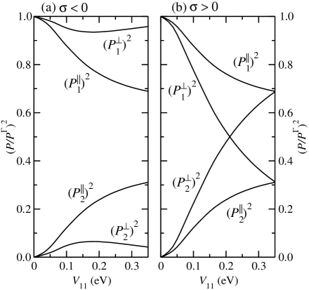
FIG. 3.: Square of momentum matrix elements [Eq. (III D)] for (a) $\sigma={\rm sgn}(V_{11}/V_{35})<0$ and (b) $\sigma>0$.

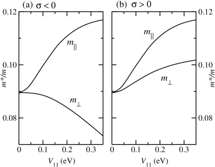
FIG. 4.: Effective masses of the lowest conduction-band state $\bar{\Gamma}_{1\text{c}}(\Gamma_{1\text{c}})$ for (a) $\sigma={\rm sgn}(V_{11}/V_{35})<0$ and (b) $\sigma>0$.

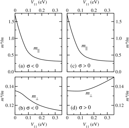
FIG. 5.: Effective masses of the second-lowest conduction-band state $\bar{\Gamma}_{1\text{c}}(\text{L}_{1\text{c}})$ for (a) and (b) $\sigma={\rm sgn}(V_{11}/V_{35})<0$, and (c) and (d) $\sigma>0$.

TABLE I.: Energies, effective masses, and momentum matrix elements or remote bands contribution, respectively, for $\Gamma_{1\text{c}}$, $\text{L}_{1\text{c}}$, and $\text{L}_{3\text{v}}$. The energy zero is the valence-band maximum $\Gamma_{5\text{v}}$.

State	Energy	Effective mass	Matrix element
	(eV)	($m$)
$\Gamma_{1\text{c}}$	$E^{\Gamma}_{\text{c}}=2$.024	$m^{\Gamma}=0$.0899	$P^{\Gamma}=8$.83 eVÅ
$\text{L}_{1\text{c}}$	$E^{\text{L}}_{\text{c}}=2$.250	$m^{\text{L}}_{\perp}=0$.1349	$P^{\text{L}}=8$.88 eVÅ
		$m^{\text{L}}_{\parallel}=1$.699	$G=-1$.57 eVÅ2
$\text{L}_{3\text{v}}$	$E^{\text{L}}_{\text{v}}=-0$.978

REFERENCES

- [1] Electronic mail: stubner@physik.uni-erlangen.de.
- [2] E. O. Kane, in Semiconductors and Semimetals, edited by R. K. Willardson and A. C. Beer (Academic Press, New York, 1966), Vol. 1, p. 75.
- [3] J. Callaway, in Quantum Theory of the Solid State (Academic Press, New York, 1974), Chap. 4.1.2 The Method.
- [4] J. M. Luttinger and W. Kohn, Phys. Rev. 97, 869 (1955).
- [5] W. Kohn, Solid State Phys. 5, 257 (1957).
- [6] G. Bastard, Wave mechanics applied to semiconductor heterostructures (Les Editions de Physique, Les Ulis, 1988).
- [7] D. M. Wood and A. Zunger, Phys. Rev. B 53, 7949 (1996).
- [8] A. Franceschetti, S.-H. Wei, and A. Zunger, Phys. Rev. B 52, 13992 (1995).
- [9] A. Gomyo, T. Suzuki, and S. Iijima, Phys. Rev. Lett. 60, 2645 (1988).
- [10] A. Zunger and S. Mahajan, in Handbook of Semiconductors, 2 ed., edited by S. Mahajan (North-Holland, Amsterdam, 1994), Vol. 3b, Chap. 19, p. 1399.
- [11] S.-H. Wei and A. Zunger, Phys. Rev. B 39, 3279 (1989).
- [12] S.-H. Wei and A. Zunger, Phys. Rev. B 57, 8983 (1998).
- [13] B. Fluegel, Y. Zhang, H. M. Cheong, A. Mascarenhas, J. F. Geisz, J. M. Olson, and A. Duda, Phys. Rev. B 55, 13647 (1997).
- [14] R. L. Forrest, T. D. Golding, S. C. Moss, Z. Zhang, J. F. Geisz, J. M. Olson, A. Mascarenhas, P. Ernst, and C. Geng, Phys. Rev. B 58, 15355 (1998).
- [15] M. E. Raikh and E. V. Tsiper, Phys. Rev. B 49, 2509 (1994).
- [16] Y. Zhang and A. Mascarenhas, Phys. Rev. B 51, 13162 (1995).
- [17] P. Ernst, Y. Zhang, F. A. J. M. Driessen, A. Masarenhas, E. D. Jones, C. Geng, F. Scholz, and H. Schweizer, J. Appl. Phys. 81, 2814 (1997).
- [18] B. A. Foreman, Phys. Rev. Lett. 80, 3823 (1998).
- [19] Note that we have used lower case letters (, , , etc.) in the above discussion to denote quantities in standard theory and upper case letters (, , , etc.) to denote the corresponding quantity in our generalized theory.
- [20] G. L. Bir and G. E. Pikus, Symmetry and Strain-Induced Effects in Semiconductors (Wiley, New York, 1974).
- [21] G. F. Koster, J. O. Dimmock, R. G. Wheeler, and H. Statz, Properties of the Thirty-Two Point Groups (MIT Press, Cambridge, Massachusetts, 1963).
- [22] P. Emanuelsson, M. Drechsler, D. M. Hofmann, B. K. Meyer, M. Moser, and F. Scholz, Appl. Phys. Lett. 64, 2849 (1994).
- [23] J.-M. Jancu, R. Scholz, F. Beltram, and F. Bassani, Phys. Rev. B 57, 6493 (1998).
- [24] M. Cardona, J. Phys. Chem. Solids 24, 1543 (1963); 26, 1351(E) (1965).
- [25] privat communication T. Kippenberg.
- [26] T. Kippenberg, J. Krauss, J. Spieler, P. Kiesel, G. H. Döhler, R. Stubner, R. Winkler, O. Pankratov, and M. Moser, Phys. Rev. B 60, 4446 (1999).
- [27] S.-H. Wei, A. Franceschetti, and A. Zunger, Phys. Rev. B 51, 13097 (1995).
- [28] Note that the value of in Ref. [26] differs from the value here, though this has only a marginal effect for our application.
- [29] P.-O. Löwdin, J. Chem. Phys. 19, 1396 (1951).
- [30] S.-H. Wei and A. Zunger, Phys. Rev. B 49, 14337 (1994).
- [31] S.-H. Wei and A. Zunger, Appl. Phys. Lett. 64, 1676 (1994).