Spin twists, domain walls,
and the cluster spin-glass phase of weakly doped cuprates

Abstract

We examine the role of spin twists in the formation of domain walls, often called stripes, by focusing on the spin textures found in the cluster spin glass phases of ${\rm La_{2-x}Sr_{x}CuO_{4}}$ and ${\rm Y_{1-x}Ca_{x}Ba_{2}Cu_{3}O_{6}}$. To this end, we derive an analytic expression for the spin distortions produced by a frustrating bond, both near the core region of the bond and in the far field, and then derive an expression for interaction energies between such bonds. We critique our analytical theory by comparison to numerical solutions of this problem and find excellent agreement. By looking at collections of small numbers of such bonds localized in some region of a lattice, we demonstrate the stability of small “clusters” of spins, each cluster having its own orientation of its antiferromagnetic order parameter. Then, we display a domain wall corresponding to spin twists between clusters of locally ordered spins showing how spin twists can serve as a mechanism for stripe formation. Since the charges are localized in this model, we emphasize that these domain walls are produced in a situation for which no kinetic energy is present in the problem.

I Introduction:

The now frequent experimental observations of spin and/or charge modulations in the cuprate superconductors and related doped transition metal oxides [2] was predicted by the “frustrated phase separation” phenomenology of Emery and Kivelson. Their theoretical considerations [3] involved the assertion that a doped Mott insulator phase separates as a consequence of the competition between the kinetic energy of mobile holes and the magnetic energies of an antiferromagnetic (AFM) phase with long-range correlations. While it seems unlikely that this scenario is correct in the strong correlation limit [4], when one adds the Coulomb interaction into this problem Emery and Kivelson argued that macroscopic phase separation became “frustrated”, and the resulting anomalous normal state possessed low-energy fluctuations corresponding to stripes, or domain walls [5]. To connote that these entities correspond to metallic stripes, it is now common to refer to these structures as “rivers of charge” [6].

Recent neutron scattering studies [7] of the single-layer La_2-xSr_xCuO₄ (LSCO) system have revealed that (at least in experimental results to date) an elastic magnetic response associated with static stripe-like correlations are only found in (i) low $x$ systems ($x\lesssim 0.06$) at low temperatures such that the transport is that of a doped semiconductor [8], and (ii) in the famous $x\approx 1/8$ system. One could interpret both the strongly disordered, low temperature results, and the $x\approx 1/8$ data, as evidence that pinning effects are necessary, either from disorder or commensurability interactions, to produce static stripes. Such arguments are consistent with the successful approach of Tranquada and coworkers in producing static stripes that could then be observed in scattering experiments in a variety of systems [2].

The low $x$, low temperature region of the LSCO phase diagram in which the static magnetic stripe correlations are found corresponds to the spin-glass phase of LSCO. Early magnetic resonance work on this system [9] suggested that it is appropriate to think of this phase as a cluster spin glass, so named because small clusters of spins achieve their own short-range AFM correlations, but the cluster-cluster ordering is spin-glass like. A numerical simulation of this phase, coupled with new crystals and new susceptibility data, lended support to this characterization [10].

In the latter paper [10], one conundrum associated with the mechanism behind the formation of the cluster spin glass phase was pointed out, and goes as follows: The frustrated phase separation phenomenology claims that support for such physics is found in the existence of the cluster spin glass phase [5]. However, detailed analysis of the transport in this region of the LSCO phase diagram concludes that the transport is similar to that of a doped semiconductor [8]. Thus, at least in the low-temperature cluster spin-glass phase the competition between kinetic and magnetic energies does not exist in the form proposed originally by Emery and Kivelson, and the question can then be asked, does the absence of the holes’ kinetic energy from extended states not eviscerate the frustrated phase separation phenomenology as a viable mechanism associated with the formation of the cluster spin glass phase? Put another way, the numerical simulations of Ref. [10] that found evidence for the character of the spin-glass phase being like that of a cluster spin glass produced this spin texture with zero kinetic energy, and thus is the kinetic energy a necessary ingredient in the formation of stripe phases [11]?

This question becomes more important in view of recent experiments of Julien, et al. [12]. These NMR/NQR results demonstrated the existence of a so-called charge glass at higher temperatures, followed by the appearance of the superconducting phase at lower temperatures, followed by the cluster spin glass phase at the lowest temperatures. The frustrated phase separation phenomenology predicts this sequence of charge glass/cluster spin glass phases, and thus unlike the above arguments, suggests that the cluster spin glass is stabilized by the pinning of the charge stripes by defects, followed by the subsequent freezing of the spin degrees of freedom within clusters defined by the pinned stripes of the charge glass phase. Unfortunately, again, the transport of this system at low temperatures is insulating (for, say, $T<75~{}K$), so in the spin glass phase there are no rivers of charge which could “carve out” the domain walls of the cluster spin glass phase!

In this manuscript we present analytical results that formalizes the claim that via quenched disorder from the Sr impurities one can produce the topology of pinned stripes without any kinetic energy. To this end, we derive the spin distortion pattern produced by such quenched disorder (which frustrates the background AFM order), and then demonstrate that this theory successfully predicts the stability of localized clusters of AFM correlated spins produced in a situation with zero kinetic energy. In this case, the origin of the stripes associated with the domain walls comes from the spin twists between the clusters, the clusters themselves having been produced by spin twists of the spin texture as the background spins attempt to accommodate the frustrating magnetic interactions produced by the quenched disorder. A well known extrapolation to higher temperatures [13] then implies that the qualitatively identical spin twists generated by mobile carriers must be part of the mechanism associated with the formation of stripes.

We wish to make clear that our paper does not claim to be the first to propose that magnetic interactions in general, and spin twists in particular, are important in the formation of stripes. Firstly, the work of Salem and one of us [14] investigated the problem of frustrating FM bonds whose locations could be chosen such that the ground-state energy was minimized. It was found that when quantum fluctuations were included, if the magnitude of the frustrating interaction was smaller than that of the background majority spins, periodic stripes of frustrating bonds were the ground state configuration. (So, in these ground states, again there is no kinetic energy but stripe phases are indeed encountered.) Secondly, when the frustrating bonds cannot chose their (static) positions but are fixed by the Sr impurity ions, the numerical simulations (mentioned above) of Ref. [10] suggested the presence of domain walls between the clusters of the cluster spin-glass phase. More recently, work of Stojkovic and coworkers [15] examined a version of the mobile hole problem by implementing a purely magnetic model that included the long-ranged spin twists produced by mobile holes (as well as the frustrating Coulombic energy between the carriers) and found many of the magnetic structures encountered in [14], including stripe phases. Lastly, White and Scalapino, who find evidence for stripe structures in the $t$–$J$ model for mobile holes [16], note that the charge and spin distributions of striped structures attempt to accommodate the frustration (read: spin twists) on the magnetic background produced by the mobile holes.

Looking at the totality of the evidence in this and the above-mentioned papers we believe that one can make a strong case that there is a similar mechanism at work in the formation of stripes in all of these situations, and that this mechanism is spin twists.

Our paper is organized as follows. In the next section we present a detailed theoretical analysis of the effects of quenched disorder on the spin texture in systems such as weakly doped LSCO, producing a reliable analytical theory of the spin distortions both near the frustrating bond and in the far field. We use this distortion field to produce an accurate interaction functional between pairs of such bonds, which we then use to demonstrate the stability of such clusters in the cluster spins glass phase. In particular, this leads to a clear identification of the local AFM order parameter of each cluster. Finally, we show the resulting spin texture between two such clusters, and demonstrate how (local) stripe configurations can be stabilized in the cluster spin-glass phase.

II Core solution and energies of the single bond problem:

A Hamiltonian and definitions

We consider the familiar model of magnetism in the CuO planes of the high $T_{\text{c}}$ cuprates in which the copper ions and oxygen holes are treated as a lattice of spins governed by a Heisenberg Hamiltonian

$$H=-\sum_{\langle ij\rangle}J_{ij}{\bf S}_{i}\cdot{\bf S}_{j}$$ (1)

where $\langle ij\rangle$ denotes a summation over near neighbour pairs of spins and the $J_{ij}$ are the exchange interaction integrals. For an undoped lattice these spins are the Cu spins and the exchange integrals are equal and negative; the ground state corresponds to an AFM ordered state on a square lattice. In what follows we simplify our considerations by using classical spins, implying that only the transverse (viz., moment reorientation) and not the longitudinal (viz., moment magnitude) spin-spin interactions are included [13].

The simplest model of the effects of doping in weakly doped cuprates at low temperatures was proposed by Emery, and corresponds to localizing the holes on oxygen sites and replacing the AFM Cu-Cu superexchange for this occupied bond with an effective FM exchange. The phase diagram of the multiply doped version of this model was produced by Aharony, et al [17]. Although detailed transport analysis of this part of the LaSrCuO phase diagram [8] has shown that a slightly different model [18, 10] of the localized dopants is required for a direct comparison to experiments, the FM bond model (which we shall refer to as the frustrating bond model) is more amenable to analytical study, for reasons that we shall elaborate on below, and shall be used throughout this paper.

Thus, we consider the Hamiltonian of Eq. (1) wherein the $i,j$ label sites of a square lattice (that is, only the Cu spins and the effective interactions between them are considered) and the exchange interaction integral between two adjacent sites $i$ and $j$ has the form

$$J_{ij}=\left\{\begin{array}[]{ll}\lambda J&\mbox{with probability $x/2$}\\ -J&\mbox{with probability $1-x/2$}\end{array}\right.$$ (2)

where $J$ and $\lambda$ are positive constants and $\lambda$ represents the relative strength of the ferromagnetic and antiferromagnetic bonds [19]. The doping level $x$ could be, say, either the Sr doping level in ${\rm La_{2-x}Sr_{x}CuO_{4}}$ or the Ca doping level in ${\rm Y_{1-x}Ca_{x}Ba_{2}Cu_{3}O_{6}}$ (noting that Neidermayer et al. [20] has shown that the phase diagrams in these two systems are identical). If we now choose a coordinate system such that linear combinations of $x$- and $y$-directed unit vectors span the lattice, then the Hamiltonian can be written explicitly as

$$H=-\frac{1}{2}\sum_{i}\sum_{\hat{a}}J_{i,i+\hat{a}}{\bf S}_{i}\cdot{\bf S}_{i+\hat{a}}$$ (3)

where $i$ is summed over all lattice sites and $\hat{a}$ ranges over $\pm\hat{x},\pm\hat{y}$. The equilibrium condition corresponds to that of zero torque from the local effective field at each lattice site:

$$\sum_{\hat{a}}J_{i,i+\hat{a}}{\bf S}_{i}\times{\bf S}_{i+\hat{a}}=0\>.$$ (4)

As is well known, the complication of treating a bipartite lattice (labelling the two sublattices as A and B sites) can be avoided by transforming the physical problem of FM bonds in a predominantly AFM background into the mathematically equivalent problem of AFM bonds in a FM background. These two pictures can be converted one to the other under the simple transformation (AFM $\rightarrow$ FM) given below:

$$J_{ij} \mapsto -J_{ij}$$ (5)

$${\bf S}_{i} \mapsto \left\{\begin{array}[]{ll}+{\bf S}_{i}&\mbox{for $i\in A$}\\ -{\bf S}_{i}&\mbox{for $i\in B$}\end{array}\right.\>.$$ (8)

Lastly, we note that the objects under consideration are classical spins, and we set their length to be one, scaling $J$ to be $JS^{2}$. Further, the ground states that we discuss in this paper all correspond to situations in which the spins lie in some plane, and thus from now on we restrict our formalism to describe planar spins. We denote the bulk direction of the spins by ${\bf S}_{\infty}$, and at any lattice site $i$ there exists a spin ${\bf S}_{i}$ characterized by the angle $\psi_{i}$ between the spin and the $x$-axis:

$${\bf S}_{i}=\hat{x}\cos\psi_{i}+\hat{y}\sin\psi_{i}~{}\Rightarrow~{}{\bf S}_{i}\cdot{\bf S}_{j}=\cos\,(\psi_{i}-\psi_{j})\>.$$ (9)

We choose $\psi_{i}=\phi_{i}+\psi_{\infty}$ where $\psi_{\infty}$ is taken to be the average angle of the spins over the bulk of the material. That is ${\bf S}_{\infty}=\hat{x}\cos\psi_{\infty}+\hat{y}\sin\psi_{\infty}$ so that the angle $\phi_{i}$, defined according to $\cos\phi_{i}={\bf S}_{i}\cdot{\bf S}_{\infty}$, represents the deviation of the spin at site $i$ from the bulk direction. The collection $\{\phi_{i}\}$ of the spin distortions at each lattice site constitutes the spin texture on the lattice.

The numbering scheme for the lattice sites near the frustrating bond (what from now on we call the bond sites) is shown in Fig. 1.

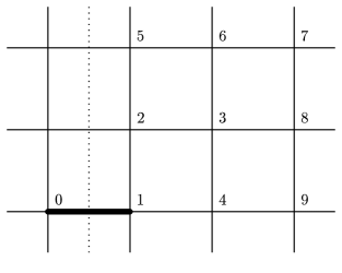
FIG. 1.: The lattice site numbering scheme. The frustrating bond sits between the 0 and 1 sites.

B Spin deviations of a frustrating bond

In a FM lattice doped with a single AFM bond, the ground state solution to the spin texture is no longer obvious, and such a situation is called frustrated. We wish to produce an accurate analytical solution to this problem in both the far-field region and close to the frustrating bond. This will allow us to accurately track the energies of both the single and many bond problems.

Consider a purely FM lattice frustrated by the introduction of an $x$-directed AFM bond between the $(0,0)$ and $(1,0)$ lattice sites. We shall denote the spin distortions at these sites by $\phi_{0}$ and $\phi_{1}$, respectively. The Hamiltonian is then written as

$$H=-J{\sum_{\langle ij\rangle}}^{\prime}\cos\,(\phi_{i}-\phi_{j})+\lambda J\,\cos\,(\phi_{0}-\phi_{1})$$ (10)

where the prime indicates the omission of the AFM bond from the summation. It is no longer clear that the trivial solution $\phi_{i}=0$ represents the ground state since there may be another solution with $\pi/2<|\phi_{0}-\phi_{1}|<3\pi/2$ that the takes the system to a lower energy state.

As is well known, considerable information can be gained from an examination of the dynamical properties of a linearized system of equations of motion about a proposed equilibrium structure. Here, we briefly outline this formalism, since it will be important to our later work. For our purposes, the dynamical behaviour of a lattice of $n$ independent spins is modeled sufficiently by

$$\ddot{\phi_{i}}=-\sum_{\hat{a}}\sin\,(\phi_{i}-\phi_{i+\hat{a}})\ \ \ i=1,2,\ldots,n\>.$$ (11)

Close to the ordered equilibrium state $\phi_{i}=0$, this behaviour is governed by the linearized system $\ddot{{\bf x}}=-M{\bf x}$ where $M=Df({\bf 0})$ is the derivative matrix of $f$ evaluated at the origin and ${\bf x}$ is related to the spin texture according to the row vector ${\bf x}^{T}=[\phi_{1},\phi_{2},\phi_{3},\ldots,\phi_{n}]$.

Solving for the normal modes, and taking note of negative eigenvalues, the instability of the system to a non FM ordered ground state can be identified. This technique, when applied for larger and larger systems, reproduces the known result [21] that an instability is first reached at $\lambda_{c}=1$ and that there is only one stable spin texture for all $\lambda$ exceeding $\lambda_{c}$.

Unlike such instability analysis, or the Fourier-based approach of Vanninemus, et al. [21], here we wish to develop a continuum theory capable of describing an infinite lattice including the spins in the immediate neighbourhood of the frustrating bond. To this end, we proceed as follows.

Let $\phi$ be a function of a continuous variable ${\bf r}$ which ranges over the entire $xy$-plane such that $\phi_{i}\mapsto\phi({\bf r}_{i})$. Then, provided that $\phi$ is a smooth, slowly varying function of position, we may approximate the equilibrium condition for the undoped system (to lowest order [22]) by

$$\nabla^{2}\phi=0\>.$$ (12)

Now consider a FM lattice frustrated by the introduction of a single $x$-directed AFM bond. The equilibrium spin distortions away from the core of the frustration are governed by Laplace’s equation. Choose the origin of the coordinate system centred on the bond, and solve Laplace’s equation, in polar coordinates, by separation of variables. The imposition of the appropriate solution symmetries [23] yields

$$\phi(r,\theta)=\sum_{m=1,3,5,\dots}^{\infty}r^{-m}A_{m}\cos m\theta\>$$ (13)

where we have adopted the convention that summations are over odd indices only.

It is clear that for sufficiently large $r$, the lowest order term dominates. That is to say, far from the bond the distortions are dipolar:

$$\phi({\bf r})=\frac{{\bf p}\cdot{\bf r}}{r^{2}}$$ (14)

where ${\bf p}=A_{1}\hat{x}$ or ${\bf p}=A_{1}\hat{y}$. This agrees with the well known results in the literature (see, e.g., Refs. [21, 17]). Unfortunately this result is inadequate for our purposes, since we also require the spin distortions near the bond. As we show below, a previous attempt [24] fails, and thus we present new arguments leading to a valid solution close to and far away from the frustrating bond. Other work has been unable to solve analytically this part of the frustrating bond problem [25] (although it is clear that they are aware of the issues that we have finally solved).

We have written down a general solution to the static spin texture on the infinite lattice due to a single AFM bond, and that solution consists of a linear combination of an infinite number of possible solution modes. However, since we have shown that the single bond system has only one stable solution, we expect that any prepared state will decay into the state of lowest energy given by the $m=1$ solution in Eq. (13). That is every $A_{m}\rightarrow 0$ for $m\neq 1$. Nonetheless, we run into the difficulty that the field equation to which Eq. (13) is a solution is not strictly valid at the bond sites. Consequently, we cannot expect that these solutions will perform well near the bond itself. Indeed, we find that the purely dipolar solution with $1/r$ fall-off fits numerical solutions extremely well $(\sim 0.5\%)$ up to three or four lattice sites away from the bond, but that in the core of the frustration the deviation becomes quite large. At the bond sites themselves, the error is $\sim 25\%$.

We may ask, of course, why such a description does not suffice if, for the most part, we are interested in the spin distortions away from the bond. Surely we can tolerate a small error at a handful of lattice sites? The answer is that we cannot. Since the spin distortions are most severe in the immediate vicinity of the bond, the spins in the core of the frustration are a large contributor to the magnitude of the total energy stored in the distortions. Thus a proper calculation of the energy in the system requires that we model the core correctly. Equally important is that, for a given solution mode, the local equilibrium condition at the bond site determines the overall magnitude of the spin distortions. That is, it fixes the magnitude of the dipole moment associated with the distortion field. Kovalev and Bogdan, who suggested a continuum approach for the core region of this problem [24], fall into precisely this trap and hence obtain the wrong magnitude for the long range behaviour for the spin distortions (see below).

It remains to be answered how we might treat the spin distortions around the bond. Ideally, we would like to treat the AFM character of the interaction in the core as a small perturbation on the field equations, but this is not possible since the continuum formalism is badly behaved at the origin under the symmetries we have imposed. A second possibility would be to derive a separate discrete solution valid in the core and to match it smoothly onto the exterior continuum solution. However, we are inclined to avoid such a patch-work approach. Not only is it somewhat inelegant, but it also defeats the purpose of introducing the continuum formalism, namely, to do away with discrete calculations altogether.

Instead, we make use of the fact that the sets $\{\cos(m\theta)/r^{m}\}$ and $\{\sin(m\theta)/r^{m}\}$ are complete (in the sense that any static spin texture satisfying the symmetries [23] specified by a single $x$- or $y$-directed bond can be expanded in one of these bases). Thus, to solve for the spin distortions everywhere on the lattice is essentially to fix the values of the coefficients $\{A_{m}\}$. In the following, we attempt to expand the solution to the spin distortions of an $x$-directed AFM bond near the origin in the basis $\{\cos(m\theta)/r^{m}\}$.

To start, we expect that the coefficient $A_{1}$ must dominate the others since $\cos(\theta)/r$ is the mode of lowest energy. Further, convergence at the bond sites requires that $(A_{m})\rightarrow 0$ faster than $2^{-m}$ as $m\rightarrow\infty$. Thus, it is meaningful to treat the expansion $\phi^{(n)}(r,\theta)$, consisting of the first $n$ terms of Eq. (13) as an approximate solution. We can then apply the local equilibrium condition at $n$ sites around the bond to determine the $n$ coefficients.

For concreteness, consider the four term expansion

$$\phi(r,\theta)=\phi^{(4)}(r,\theta)=A_{1}\frac{\cos\theta}{r}+A_{3}\frac{\cos 3\theta}{r^{3}}+A_{5}\frac{\cos 5\theta}{r^{5}}+A_{7}\frac{\cos 7\theta}{r^{7}}\>.$$ (15)

To solve for its four coefficients we require the $9\times 4$ transformation matrix

$$T:={\left[\frac{\partial\phi_{i}}{\partial A_{j}}\right]}_{9\times 4}=\left[\begin{array}[]{cccc}2&8&32&128\\ \\ \frac{2}{5}&-\frac{88}{125}&\frac{1312}{3125}&\frac{3712}{78125}\\ \\ \frac{6}{13}&-\frac{72}{2197}&-\frac{19104}{371293}&-\frac{569472}{62748517}\\ \\ \frac{2}{3}&\frac{8}{27}&\frac{32}{243}&\frac{128}{2187}\\ \\ \frac{2}{17}&-\frac{376}{4913}&\frac{35872}{1419857}&-\frac{2566016}{410338673}\\ \\ \frac{6}{25}&-\frac{936}{15625}&-\frac{7584}{9765625}&\frac{9784704}{6103515625}\\ \\ \frac{10}{41}&-\frac{920}{68921}&-\frac{335200}{115856201}&\frac{609920}{194754273881}\\ \\ \frac{10}{29}&\frac{520}{24389}&-\frac{47200}{20511149}&-\frac{14926720}{17249876309}\\ \\ \frac{2}{5}&\frac{8}{125}&\frac{32}{3125}&\frac{128}{78125}\end{array}\right]$$ (16)

(generated using a symbolic algebra computer package) and the matrix

$$M=\left[\begin{array}[]{rrrrrrrrr}(3-2\lambda)&-2&0&-1&0&0&0&0&0\\ -1&5&-1&0&-1&0&0&0&0\\ 0&-1&4&-1&0&-1&0&-1&0\\ -1&0&-2&4&0&0&0&0&-1\\ \end{array}\right]$$ (17)

of linearized equilibrium conditions at sites 1 through 4. Defining the row vector ${\bf a}^{T}=[A_{1},A_{3},A_{5},A_{7}]$ the determination of $\{A_{m}\}$ is equivalent to solving the homogeneous system of equations $MT{\bf a}=0$. The requirement that $\det(MT)=0$ yields a critical value $\lambda_{\text{c}}\,\dot{=}\,1.0113$ (very close to the true value $\lambda_{\text{c}}=1$) for which

$${\bf a}=[0.5987,0.0742,0.1960,-0.0552]\times\phi_{1}\>.$$ (18)

That is to say, the best four term expansion reads

$$\phi^{(4)}(r,\theta) = \phi(r,\theta)=A_{1}\frac{\cos\theta}{r}+A_{3}\frac{\cos 3\theta}{r^{3}}+A_{5}\frac{\cos 5\theta}{r^{5}}+A_{7}\frac{\cos 7\theta}{r^{7}}$$ (19)

$$= \frac{{\bf p}\cdot{\bf r}}{r^{2}}+\sum_{m=3,5,7}A_{m}\frac{\cos m\theta}{r^{m}}$$ (20)

with

$$p=|{\bf p}|=A_{1}=+0.5987\phi_{1},~{}A_{3}=+0.0742\phi_{1},A_{5}=+0.1960\phi_{1},~{}A_{7}=-0.0552\phi_{1}$$ (21)

The coefficients of $\phi^{(n)}(r,\theta)$ for $n$ being increased from 1 to 4 are presented in Table I.

TABLE I.: Spin distortion amplitudes of $\phi^{(n)}(r,\theta)$ for $n=1,2,3,4$.

$n$	$\lambda_{\text{c}}$	$A_{1}/\phi_{1}$	$A_{3}/\phi_{1}$	$A_{5}/\phi_{1}$	$A_{7}/\phi_{1}$
1	17/15	15/22	-	-	-
2	1.0222	0.6274	-0.0318	-	-
3	1.1551	0.3516	-0.1220	0.0398	-
4	1.0113	0.5987	0.0742	0.1960	-0.0552

What this calculation provides that the other does not is the value of the multiplicative factor $\partial A_{1}/\partial\phi_{1}=A_{1}/\phi_{1}\sim 0.6$ relating the magnitude of the spin distortions at the bond sites to the magnitude of the dipole moment associated with the bond itself.

We have shown that the spin distortions are given everywhere by

$$\phi(r,\theta)=A_{1}\frac{\cos\theta}{r}+A_{3}\frac{\cos 3\theta}{r^{3}}+A_{5}\frac{\cos 5\theta}{r^{5}}+\cdots$$ (22)

As we have seen, however, this expression is unwieldy in that it requires the application of infinitely many local equilibrium conditions to fully determine the coefficients $\{A_{m}\}$. Even to calculate the coefficients of a finite series expansion of several terms is computationally expensive. Ideally, what we would like to have is a solution dependent on a single parameter whose value is determined by applying a single boundary condition at the bond itself. Here we now outline such a method. We find that a simple assumption on the distribution of modes can provide this very result.

We proceed by assuming that the spectrum of modes can be modeled by

$$A_{2n+1}=(-1)^{n}\frac{2A_{1}}{(2n+1)2^{2n+1}}$$ (23)

or, in somewhat simplified notation,

$$A_{k}=(\pm)\frac{2A_{1}}{k2^{k}}$$ (24)

where the index $k$ is taken to be odd and the sign is taken alternately positive and negative. This form falls off just fast enough to make the series converge — besides this seemingly naive reason, we appeal to its success (described in detail below) to justify its usage.

Under this assumption

$$\phi(r,\theta) = A_{1}\frac{\cos\theta}{r}+A_{3}\frac{\cos 3\theta}{r^{3}}+A_{5}\frac{\cos 5\theta}{r^{5}}+\cdots$$ (25)

$$= 2A_{1}\left(\frac{\cos\theta}{2r}-\frac{1}{3}\frac{\cos 3\theta}{(2r)^{3}}+\frac{1}{5}\frac{\cos 5\theta}{(2r)^{5}}-\cdots\right)\>.$$ (26)

Now, the magnitude of the dipole moment in terms of the distortion at the bond site follows immediately from solving $\phi(1/2,0)=\phi_{1}$ self-consistently. We find that $A_{1}=\frac{2}{\pi}\phi_{1}$ and hence

$$\phi(r,\theta)=\phi_{1}\frac{4}{\pi}\sum_{k}(\pm)\frac{\cos k\theta}{k(2r)^{k}}$$ (27)

since

$$\phi_{1}=\phi(1/2,0)=\phi_{1}\frac{4}{\pi}\left(1-\frac{1}{3}+\frac{1}{5}-\cdots\right)$$ (28)

which is identically equal to $\phi_{1}$. The spin distortions at the remaining sites in the immediate neighbourhood of the bond are as follows:

$$\phi_{2}=\phi(\sqrt{5}/2,\arctan(2))=0.2951672353\phi_{1}~{},~{}\phi_{4}=\phi(3/2,0)=0.4096655294\phi_{1}$$ (29)

(In fact, one may prove the identity $2\phi_{2}+\phi_{4}\equiv\phi_{1}$, which we shall use later on in this paper.)

Notice that as $r$ becomes large, we get

$$\phi(r,\theta) \rightarrow \phi_{1}\frac{4}{\pi}\cos\theta\arctan\left(\frac{1}{2r}\right)\rightarrow\phi_{1}\frac{4}{\pi}\frac{\cos\theta}{2r}$$ (30)

$$= \phi_{1}\frac{2}{\pi}\frac{\cos\theta}{r}$$ (31)

so that the solution retains its familiar long range behaviour. That is

$$\phi({\bf r})=\frac{{\bf p}\cdot{\bf r}}{r^{2}}$$ (32)

but now with

$$p=|{\bf p}|=\frac{2}{\pi}\phi_{1}\>.$$ (33)

What remains is to determine the parameter $\phi_{1}$. As promised, the bond furnishes a single boundary condition in the form of the equilibrium condition applied at either of the bond sites:

$$-\lambda\sin(2\phi_{1})+2\sin(\phi_{1}-\phi_{2})+\sin(\phi_{1}-\phi_{4})=0\>.$$ (34)

This is an implicit equation for $\phi_{1}$, and thus for all of the spin distortions as a function of $\lambda$. Its solution is plotted in Fig. 2.

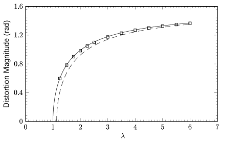
FIG. 2.: The distortion magnitude as a function of the frustrating AFM bond strength $\lambda$. The solid line represents the prediction of our analytical theory, and the broken line is the prediction based on the solution of Kovalev and Bogdan [24]. Open squares are numerically generated data points from large lattices (from $40\times 39$ up to $80\times 79$ lattices) with converged numerical solutions for this quantity.

Moreover, the linearized equation gives

$$-\lambda_{\text{c}}2\phi_{1}+2(\phi_{1}-\phi_{2})+(\phi_{1}-\phi_{4})=0$$ (35)

which can be solved explicitly:

$$\lambda_{\text{c}}=\frac{3}{2}-\frac{2\phi_{2}+\phi_{4}}{2\phi_{1}}\equiv 1\>.$$ (36)

That is, our ansatz correctly reproduces the exact critical value of $\lambda_{c}$ !

A comparison of the solution Eq. (27) to numerical simulations is presented in Fig. 3; clearly, the agreement is excellent, providing the most direct support for our ansatz.

FIG. 3.: The local spin distortions as a function of distance along the $x$-axis for an $x$-directed AFM bond. The solid line represents the function $\phi(r,0)$ described in the text. Open squares are converged numerically generated data points from simulations performed on the same size lattices as in Fig. 2. The broken line is the $\phi^{(1)}(r,\theta)$ solution of Kovalev and Bogdan [24] which fails to predict quantitatively the correct dipole moment of the long-range distortions.

C Energy functional

We now calculate the total energy stored in the spin distortions induced by a single AFM bond. That these distortions are both small and slowly varying in position away from the core allows us to convert the sum of the energy contributions into an integral of the energy density $(\nabla\phi)^{2}$. A complete derivation is provided in Appendix A, and we summarize the results below.

To begin, the Hamiltonian is approximated to second order everywhere except across the AFM bond itself:

$$H\approx-\sum_{\langle ij\rangle}J_{ij}+\frac{1}{2}J{\sum_{\langle ij\rangle}}^{\prime}(\phi_{i}-\phi_{j})^{2}-2\lambda J\sin^{2}\,\phi_{1}$$ (37)

Of course, the term $-\sum J_{ij}$ represents the total energy of the system in the absence of spin distortions so that the energy from the distortions alone is given by the latter two terms. They, in turn, can be expanded using the continuum approximation

$$E_{\mbox{dist}} = \frac{1}{4}J\sum_{i\neq 0,1}\sum_{\hat{a}}(\phi_{i}-\phi_{i+\hat{a}})^{2}+\frac{1}{2}J\Bigl{(}2(\phi_{1}-\phi_{4})^{2}+4(\phi_{1}-\phi_{2})^{2}\Bigr{)}-2\lambda J\sin^{2}\phi_{1}$$ (38)

$$\approx J\biggl{\{}\frac{1}{2}\int_{M}(\nabla\phi)^{2}d^{2}r+(\phi_{1}-\phi_{4})^{2}+2(\phi_{1}-\phi_{2})^{2}-2\lambda\sin^{2}\phi_{1}\biggr{\}}$$ (39)

where $M$ is the $xy$-plane excluding a small region about the bond centre.

An explicit evaluation of the energy using the solution of the previous subsection is presented in Appendix A, wherein the full effect of the core region is accounted for. We find

$$E_{\mbox{dist}}=2J\left(\phi_{1}^{2}-\lambda\sin^{2}\phi_{1}\right)\>.$$ (40)

This result is compared to numerical simulations in Fig. 4, and again, excellent agreement between our numerical solutions and our analytical work is found.

So, now we carry on to the examination of the many-bond problem, having an excellent solution to both the core and far-field distortion patterns of the single-bond problem, as well as an accurate energy functional for an isolated frustrating bond.

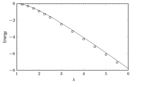
FIG. 4.: Energy of a single bond (in units of $J$) as a function of the relative AFM bond strength $\lambda$. The solid line represents the prediction of theory, and open squares are converged numerically generated data points from simulations performed on the same size lattices as in Fig. 2.

III Interacting Frustrating Bonds:

After dealing with a single bond in isolation, the next step toward treating a non-zero density of bonds is to determine how bonds interact with one another. In this subsection we consider the problem of two bonds.

Suppose that there is an AFM bond, call it $A$, between the 0 and 1 sites. Then suppose that another similarly directed bond, call it $B$, is placed between the $s$ and $s+1$ sites and that a vector ${\bf R}$ making an angle $\Phi$ with the $x$-axis connects the two bond centres, as in Fig. 5.

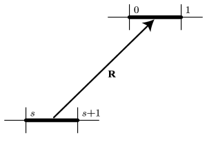
FIG. 5.: The geometry and labelling used for two parallel bonds separated by a vector ${\bf R}$.

We expect that the energy can be parametrized by two variables

$$\alpha=\frac{\phi_{1}-\phi_{0}}{2}~{}~{}~{}~{}~{}~{}~{}~{}\beta=\frac{\phi_{s+1}-\phi_{s}}{2}$$ (41)

and that it can be written in the form

$$E_{2}(\alpha,\beta) = E(\alpha)+E(\beta)+Jg\alpha\beta$$ (42)

$$= 2J(1-\lambda)(\alpha^{2}+\beta^{2})+\left(\frac{2}{3}-\delta\right)J\lambda(\alpha^{4}+\beta^{4})+Jg\alpha\beta$$ (43)

where $g=g({\bf R})$ is a real-valued function of the separation and relative orientation of the bonds and $\delta$ is a small correction representing the $4^{\mbox{th}}$ order contribution to energy from the spin distortions which were neglected in Eq. (39).

The requirement that the spin texture remain invariant up to a global sign change under interchange of $\alpha$ and $\beta$ reduces the two parameter energy expression (43) to one of two one parameter expressions $E_{2}^{+}$ or $E_{2}^{-}$ corresponding to the symmetric ($\alpha=\beta$) and the antisymmetric ($\alpha=-\beta$) state.

Case 1: $\phi=\alpha=-\beta$. In this case, the dipoles associated with the bond are anti-aligned. The total energy is

$$E_{2}^{-}(\phi)=E_{2}(\phi,-\phi)=4J\left((1-\lambda-\frac{1}{4}g)\phi^{2}+\frac{1}{2}\left(\frac{2}{3}-\delta\right)\lambda\phi^{4}\right)~{}~{}<~{}~{}2E(\phi)\>.$$ (44)

Minimization with respect to $\phi$ gives

$$\phi=\sqrt{(\lambda+\frac{1}{4}g-1)/\left(\frac{2}{3}-\delta\right)\lambda}\>.$$ (45)

This implies that the critical value of $\lambda$ at which the canted ground state first appears is lower than it is for a single AFM bond $\lambda_{c}=1$.

Case 2: $\phi=\alpha=\beta$. This represents a higher energy metastable state characterized by aligned dipoles. The energy for this configuration is

$$E_{2}^{+}(\phi)=E_{2}(\phi,\phi)=4J\left((1-\lambda+\frac{1}{4}g)\phi^{2}+\frac{1}{2}\left(\frac{2}{3}-\delta\right)\lambda\phi^{4}\right)~{}~{}>~{}~{}2E(\phi)$$ (46)

with distortion magnitude

$$\phi=\sqrt{(\lambda-\frac{1}{4}g-1)/\left(\frac{2}{3}-\delta\right)\lambda}\>.$$ (47)

Now the critical value of the coupling constant required for a distorted ground state exceeds $\lambda_{c}=1$.

Case 1 is of particular interest since it yields the ground state energy $E_{2}^{0}$ of the two bond system. Further, by re-expressing that energy in terms of the energy of a single bond (extracted from Eq. (40) in the limit $\lambda\rightarrow\lambda_{c}+0^{+}$) we can determine the energy of interaction between the two bonds.

$$E^{0}_{2}=-4J\frac{(\lambda+\frac{1}{4}g-1)^{2}}{\lambda(2/3-\delta)}=2E^{0}-J\frac{(\lambda-1)}{\lambda(2/3-\delta)}g({\bf R})-J\frac{1}{8\lambda(2/3-\delta)}g^{2}({\bf R})$$ (48)

In general, since we expect $g$ to be small, we can write

$$E_{\mbox{int}}=-J\frac{(\lambda-1)}{\lambda(2/3-\delta)}g({\bf R})\>.$$ (49)

However, as $\lambda\rightarrow 1$, we obtain

$$E_{\mbox{int}}\rightarrow-J\frac{1}{8\lambda(2/3-\delta)}g^{2}({\bf R}),$$ (50)

a weak, long-range interaction with a higher power law, a consequence of the fact that the dipolar distortions do not pre-exist in the unperturbed medium at $\lambda=1$. Such an interaction is analogous to the Van der Waals interaction between thermally fluctuating dipoles.

The function $g$ expresses the functional dependence of the interaction energy on the geometrical configuration of the bonds. We have yet to determine its exact form. All we can say now is that

$$\lim_{R\rightarrow\infty}g({\bf R})=0$$ (51)

which simply formalizes our expectation that two bonds must be non-interacting at infinite separation.

The long range spin distortions arising from each of the bonds $A$ and $B$ with dipole moments ${\bf p}^{A}$ and ${\bf p}^{B}$ is given by

$$\phi^{A}({\bf r})=\frac{{\bf p}^{A}\cdot{\bf r}}{r^{2}}\ ~{}~{}~{}\mbox{and}~{}~{}~{}\ \phi^{B}({\bf r})=\frac{{\bf p}^{B}\cdot{\bf r}}{r^{2}}\>.$$ (52)

The linearity of the Laplacian implies that the field equations admit a superposition principle. Therefore, we take the total spin distortion at each point to be

$$\phi=\phi^{A}+\phi^{B}$$ (53)

where $\phi^{A}$ and $\phi^{B}$ are the spin distortions from each bond in the absence of the other.

The energy in the distortions away from the cores goes as

$$\int_{M2}(\nabla\phi)^{2}d^{2}r = \int_{M2}\bigl{(}\nabla(\phi^{A}+\phi^{B})^{2}\bigr{)}d^{2}r$$ (54)

$$= \int_{M2}(\nabla\phi^{A})^{2}d^{2}r+\int_{M2}(\nabla\phi^{B})^{2}d^{2}r$$ (56)

$$+\int_{M2}\nabla\phi^{A}\cdot\nabla\phi^{B}d^{2}r$$

where $M2\left(={\mathbb{R}}\backslash D_{\epsilon}({\bf 0})\backslash D_{\epsilon}({\bf R})\right)$ is the $xy$-plane with disks removed about the bond centres. The last term in this expression vanishes identically, which indicates that the core of each bond interacts with the long-range spin distortions of the other and justifies a rather involved calculation of the interaction energy which we have relegated to Appendix B.

What we find is that $E_{\mbox{int}}$ has the form of a magnetic dipole interaction. Further, although in the preceding discussion we considered only parallel bonds, it is simple to show that these results hold more generally. Thus, for two bonds which are parallel or perpendicular we have

$$E_{\mbox{int}}=J\frac{2\pi}{R^{2}}\left\{2({\bf p}^{A}\cdot\hat{{\bf R}})({\bf p}^{B}\cdot\hat{{\bf R}})-{\bf p}^{A}\cdot{\bf p}^{B}\right\}\>.$$ (57)

Finally, we can work backwards to find $g({\bf R})$. For parallel bonds,

$$E_{\mbox{int}}=J\frac{2\pi}{R^{2}}\left\{2({\bf p}^{A}\cdot\hat{{\bf R}})({\bf p}^{B}\cdot\hat{{\bf R}})-{\bf p}^{A}\cdot{\bf p}^{B}\right\}=\pm J\frac{(\lambda-1)}{\lambda(2/3-\delta)}\frac{8}{\pi R^{2}}\cos 2\Phi\>.$$ (58)

That is

$$g({\bf R})=\frac{8}{\pi R^{2}}\cos 2\Phi\>.$$ (59)

We note that the identical calculation for two perpendicular bonds gives

$$g({\bf R})=\frac{8}{\pi R^{2}}\sin 2\Phi\>.$$ (60)

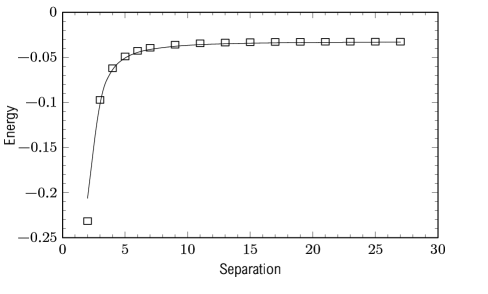
FIG. 6.: The ground state energy of two parallel bonds, for $\lambda=1.1$, at various separations along the $x$-axis, where the solid line is our prediction and the open squares are converged numerically generated data points from simulations performed on the same size lattices as in Fig. 2.

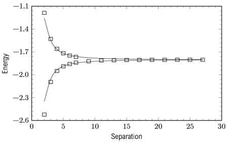
FIG. 7.: Energy of two parallel bonds, $\lambda=2$, at various separations along the $x$-axis, where the solid lines and open squares are converged numerically generated data points from simulation performed on the same size lattices as in Fig. 2. The upper curve corresponds to the metastable state with dipoles similarly directed $(\rightarrow\rightarrow)$, while the lower energy curve corresponds to oppositely directed dipoles ($\rightarrow\leftarrow)$.

IV Clusters in the cluster spin glass phase:

We should ask whether the results we have obtained so far for the one and two bond problems can be generalized to allow us to tackle the problem of a lattice frustrated by the presence of any number of arbitrarily placed AFM bonds. It should be clear that, in general, even for relatively few bonds, the induced spin distortions will be very complicated and the energy surface characterized by many closely spaced, low-lying states. In such a case one must resort to sophisticated computer algorithms to numerically generate the ground state spin texture, and the qualitative analysis of the cluster spin-glass phase from such work has been analyzed elsewhere [26, 10].

In contrast to that work, here we note that there are configurations of suitably high symmetry for which we can confidently treat the spins as planar and even solve analytically for the spin distortions and energies of all the possible states. The smallest such configuration is the square cluster of parallel bonds.

By a cluster we imply a collection of bonds arranged in some local region on the lattice. That collection, call it $C$, can be thought of as a set of dipole–position pairs: $\{({\bf p}^{\alpha},{\bf r}^{\alpha})\}_{\alpha\in C}\>.$ Given a high symmetry cluster, for which a spin-planar ground state is justified, the spin distortions away from the cores of the bonds are given by

$$\phi({\bf r})=\sum_{\alpha\in C}\frac{{\bf p}^{\alpha}\cdot({\bf r}-{\bf r}^{\alpha})}{|{\bf r}-{\bf r}^{\alpha}|^{2}}$$ (61)

which is the solution (unique for the required symmetry) to the equation

$$\nabla^{2}\phi({\bf r})=-2\pi\nabla\cdot\sum_{\alpha\in C}{\bf p}^{\alpha}\delta({\bf r}-{\bf r}^{\alpha})\>.$$ (62)

The total interaction energy of the cluster can be written as the sum of all pairwise interactions

$$E_{\mbox{int}}=\sum_{\alpha<\beta\in C}J\frac{2\pi}{|{\bf r}^{\alpha}-{\bf r}^{\beta}|^{2}}\big{(}2\frac{{\bf p}^{\alpha}\cdot({\bf r}^{\alpha}-{\bf r}^{\beta})\,{\bf p}^{\beta}\cdot({\bf r}^{\alpha}-{\bf r}^{\beta})}{|{\bf r}^{\alpha}-{\bf r}^{\beta}|^{2}}-{\bf p}^{\alpha}\cdot{\bf p}^{\beta}\big{)}\>.$$ (63)

Thus, for instance, the $L\times L$ square cluster of parallel bonds given by

$${\bf r}^{1}=(0,0),~{}~{}{\bf r}^{2}=(L,0),~{}~{}{\bf r}^{3}=(0,L),~{}~{}{\bf r}^{4}=(L,L),~{}~{}{\bf p}^{\alpha}=\pm p\hat{x}\ \ {\rm for}~{}~{}\alpha\in C=\{1,2,3,4\},$$ (64)

has a rather simple interaction energy. There are four possibilities depending on the the orientation of each dipole:

$$E_{\mbox{int}}=-J\frac{8\pi}{L^{2}}p^{2}\,,\,0\,,\,0\,,\,+J\frac{8\pi}{L^{2}}p^{2}$$ (65)

In practice, however, the degeneracy of the middle two states is lifted by higher order terms in the interaction energy. Indeed, the splitting observed in numerical simulations enables us to list the four distinguished states in order of decreasing energy.

$$\left|\begin{array}[]{cc}\rightarrow~{}~{}\rightarrow\\ \leftarrow~{}~{}\leftarrow\end{array}\right|~{}~{},~{}~{}\left|\begin{array}[]{cc}\rightarrow~{}~{}\rightarrow\\ \rightarrow~{}~{}\leftarrow\end{array}\right|~{}~{},~{}~{}\left|\begin{array}[]{cc}\rightarrow~{}~{}\rightarrow\\ \rightarrow~{}~{}\rightarrow\end{array}\right|=\mbox{first excited state}~{}~{},~{}~{}\left|\begin{array}[]{cc}\leftarrow~{}~{}\rightarrow\\ \leftarrow~{}~{}\rightarrow\end{array}\right|=\mbox{ground state}$$ (66)

The first excited state consists of four similarly directed dipoles. Destructive interference inside the cluster gives zero net distortion, but outside the cluster the dipoles add constructively so that the cluster acts like a single unit with a much stronger moment. This results in very strong long range spin distortions. Far enough from the bond, the spin distortions are given by

$$\phi({\bf r})=\frac{4{\bf p}\cdot{\bf r}}{r^{2}}\>.$$ (67)

Since the long range spin distortions mediate the interaction between bonds, we expect a cluster of this kind to strongly couple to other bonds in the lattice.

In the ground state, for which the spin distortion pattern is shown in Fig. 8, we have the opposite case: internally, the dipoles add constructively to give large distortions whereas outside they cancel to give very small ones. The absence of long range spin distortions implies that these clusters can only weakly interact with other bonds. Most interesting, though, is that the internal spins are uniformly oriented but differently ordered from those spins outside the cluster.

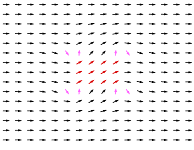
FIG. 8.: The ground state spin texture of the $4\times 4$ square cluster for four frustrating bonds. The pink spins are bond sites at which the frustrating bonds are placed. For clarity, the spins within the locally ordered cluster are coloured red.

Numerical solutions of the energies of this square cluster are shown in Fig. 9. The solid curves are our analytical results (apart from a constant times the single-bond energy (that is straightforward to calculate)), and provides strong support for their usage. In the ground state this figure makes clear that the binding energy of the cluster can be quite large, especially for small cluster sizes. Further, square clusters tend to settle into states with strong internal binding and which interact only weakly with other bonds. That is to say, a square cluster is a locally ordered domain whose local order parameter ${\bf\hat{\Omega}}$ is non-collinear with spins in the rest of the lattice. However, this behaviour is a strong function of cluster size. This construction, and the energy plot of Fig. 9, demonstrates that such clusterings of spins (in regions that are not too large) are stable.

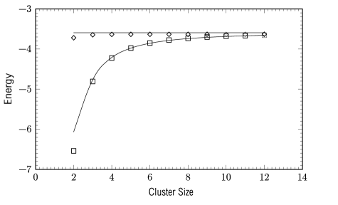
FIG. 9.: Energy of the ground (open squares and lower curve) and first excited (open diamonds and upper curve) states of the four frustrating bond arrangement described in the text. The open squares and diamonds are converged numerically generated data points from simulations performed on the same size lattices as in Fig. 2.

The relation of such clusters to stripes, or in the case of spin modulations, to the physics associated with the appearance of domain walls, can be demonstrated by considering the interface between such clusters, and to this end we have analyzed a six-bond cluster given by

$${\bf r}^{1}=(0,0),~{}~{}{\bf r}^{2} = (L,0),~{}~{}{\bf r}^{3}=(2L,0),~{}~{}{\bf r}^{4}=(0,L),~{}~{}{\bf r}^{5}=(L,L),~{}~{}{\bf r}^{6}=(2L,L),~{}~{}$$ (69)

$${\bf p}^{\alpha}=\pm p\hat{x}\ \ {\rm for}~{}~{}\alpha\in C=\{1,2,3,4,5,6\}~{}~{}.$$

Following the above analysis for four bonds, for the six-bond situation there are 64 possible choices of the dipole moments’ orientations, and these states have 15 different energies. The lowest energy configuration corresponds to

$$\left|\begin{array}[]{ccc}\rightarrow~{}~{}\leftarrow~{}~{}\rightarrow\\ \rightarrow~{}~{}\leftarrow~{}~{}\rightarrow\end{array}\right|$$ (70)

and has a dipole-pair interaction energy of $(-103\pi J/10)~{}(p/L)^{2}$ (which is noticeably lower than the first excited state, which has an energy of $(-38\pi J/10)~{}(p/L)^{2}$).

The ground state spin texture for this location of the six frustrating bonds is shown in Fig. 10. From this figure one can see the important result that this arrangement of spins is exactly what would expect if each $4\times 4$ cluster within the 6-bond cluster was in its respective ground state. Thus, between these $4\times 4$ clusters one obtains a domain wall, of width one lattice spacing, over which the local magnetic order parameter is rotated. Numerical evidence suggestive of this type of domain wall was discussed at length in Ref. [10] for the case of a random distribution (and orientation) of a non-zero density of frustrating spin interactions, and it is clear that the same physics is at work in these two situations: spin twists.

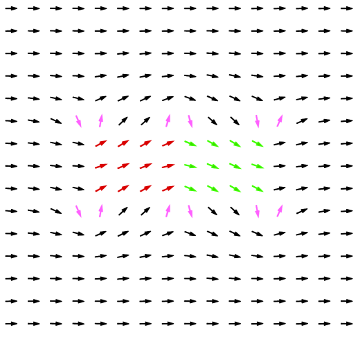
FIG. 10.: Ground state of the six frustrating bonds showing the domain wall between two clusters of locally ordered spins. As in Fig. 8, the spins of the bond sites are coloured pink, while the two clusters are coloured red and green, respectively.

V Conclusions:

The above formalism has provided a detailed analytical theory of the spin distortions generated by frustrating bonds, and of the interactions mediated by the spin background between them. We have critiqued its validity by comparing to numerical solutions, and have found excellent agreement. Then, by focusing on highly symmetrical distributions of frustrating bonds, reminiscent of local regions of bonds in the multiply doped state, we have used this theory to verify the existence of locally ordered magnetic clusters. Most importantly, our work shows that these clusters are stable. These are the clusters envisioned to exist in the so-called cluster spin-glass phase [9, 10] of LSCO and ${\rm Y_{1-x}Ca_{x}Ba_{2}Cu_{3})_{6}}$ [20].

It is to be stressed that it is believed that mobile holes produce the same kinds of spin distortions that are produced by the frustrating bonds discussed in this paper [13, 27]. Thus, we believe that our results support previous suggestions [14, 15, 16] that spin twists and distortions are part of the competing interactions that might lead to rivers of charge appearing as low-energy fluctuations in the doped cuprate systems.

A Single Bond Energy

The question of the energy stored in the spin distortions can be answered by expanding the Hamiltonian as follows:

$$H = -J{\sum_{\langle ij\rangle}}^{\prime}\cos\,(\phi_{i}-\phi_{j})+\lambda J\cos\,(\phi_{1}-\phi_{0})$$ (A1)

$$\approx -J{\sum_{\langle ij\rangle}}^{\prime}\left(1-\frac{1}{2}(\phi_{i}-\phi_{j})^{2}\right)+\lambda J\cos\,(2\phi_{1})$$ (A2)

$$= -\sum_{\langle ij\rangle}J_{ij}+\frac{1}{2}J{\sum_{\langle ij\rangle}}^{\prime}(\phi_{i}-\phi_{j})^{2}-2\lambda J\sin^{2}\,\phi_{1}$$ (A3)

Of course, the term $-\sum J_{ij}$ represents the energy intrinsic to the lattice. Therefore, the energy from the spin distortions alone is given by

$$\frac{1}{2}J{\sum_{\langle ij\rangle}}^{\prime}(\phi_{i}-\phi_{j})^{2}-2\lambda J\sin^{2}\phi_{1}\>.$$ (A4)

This in turn can be expanded using the continuum approximation

$$E_{\mbox{dist}} \approx J\biggl{\{}\frac{1}{2}\int_{M}(\nabla\phi)^{2}d^{2}r+(\phi_{1}-\phi_{4})^{2}+2(\phi_{1}-\phi_{2})^{2}-2\lambda\sin^{2}\phi_{1}\biggr{\}}$$ (A5)

$$= J\biggl{\{}\frac{1}{2}\int_{\partial M}\phi\nabla\phi\cdot{\bf ds}+(\phi_{1}-\phi_{4})^{2}+2(\phi_{1}-\phi_{2})^{2}-2\lambda\sin^{2}\phi_{1}\biggr{\}}$$ (A6)

where $M={\cal R}\backslash D_{\epsilon}({\bf 0})$ is the $xy$-plane excluding a small region about the bond centre. The integral term of this expression must be evaluated. Since the core of the bond occupies a unit disk at the origin, the appropriate value for $\epsilon$ is 1. Thus, one finds

$$E_{\mbox{dist}}=J\biggl{\{}\frac{\pi}{2}\sum_{k}kA_{k}^{2}+(\phi_{1}-\phi_{4})^{2}+2(\phi_{1}-\phi_{2})^{2}-2\lambda\sin^{2}\phi_{1}\biggr{\}}\>.$$ (A7)

Using the results for the mode characterization of Eq. (23) gives

$$\sum_{k}kA_{k}^{2}=\sum_{k}k{\left(\frac{2A_{1}}{k2^{k}}\right)}^{2}=\frac{8}{\pi^{2}}\ln\left(\frac{5}{3}\right)\phi_{1}^{2}$$ (A8)

and the identity $2\phi_{2}+\phi_{4}=\phi_{1}$ allows us to write

$$(\phi_{1}-\phi_{4})^{2}+2(\phi_{1}-\phi_{2})^{2}=\phi_{1}^{2}+2\phi_{2}^{2}+\phi_{4}^{2}\>.$$ (A9)

Thus the energy in the spin distortions is

$$E_{\mbox{dist}}=J\left\{\left(\frac{4}{\pi}\ln\left(\frac{5}{3}\right)+1\right)\phi_{1}^{2}+2\phi_{2}^{2}+\phi_{4}^{2}-2\lambda\sin^{2}\phi_{1}\right\}$$ (A10)

which can be evaluated using Eq. (29) to give

$$E_{\mbox{dist}}=2J\left(\phi_{1}^{2}-\lambda\sin^{2}\phi_{1}\right)\>.$$ (A11)

We stress that this expression includes the energy from the core of the spin distortion field.

B Interaction Energy

In accordance with Fig. 5, we write the spin distortion at the 0 site from the bond B as

$$\phi_{0}^{B}=\frac{{\bf p}^{B}\cdot({\bf R}+\frac{1}{2}\hat{x})}{|{\bf R}+\frac{1}{2}\hat{x}|^{2}}\approx{\bf p}^{B}\cdot({\bf R}+\frac{1}{2}\hat{x})\frac{1}{R^{2}}\left[1-\frac{{\bf R}\cdot\hat{x}}{R^{2}}-\frac{1}{4R^{2}}\right]\>.$$ (B1)

A similar expression can be written down for the other bond site. Then, by superposition, the difference between the net distortions at sites 0 and 1 is

$$(\phi_{0}-\phi_{1})=(\phi_{0}^{A}-\phi_{1}^{A})-\frac{2}{R^{4}}({\bf p}^{B}\cdot{\bf R})({\bf p}^{B}\cdot\hat{x})+\frac{1}{R^{2}}{\bf p}^{B}\cdot\hat{x}+{\cal O}\left(\frac{1}{R^{2}}\right)$$ (B2)

Then we make use of the relationship between the spin distortions at the bond sites and the magnitude of the dipole moment:

$$(\phi_{0}^{A}+\phi_{1}^{A})\approx 2\frac{\pi}{2}p^{A}\>.$$ (B3)

Therefore

$$(\phi_{0}-\phi_{1})^{2}=(\phi_{0}^{A}+\phi_{1}^{A})^{2}-\frac{8\alpha}{R^{4}}({\bf p}^{A}\cdot{\bf R})({\bf p}^{B}\cdot{\bf R})+\frac{4\alpha}{R^{2}}{\bf p}^{A}\cdot{\bf p}^{B}$$ (B4)

so that

$$\frac{1}{2}E=E({\bf p}^{A})+\frac{1}{2}J\left\{\frac{2\pi}{R^{2}}{\bf p}^{A}\cdot{\bf p}^{B}-\frac{4\pi}{R^{4}}({\bf p}^{A}\cdot{\bf R})({\bf p}^{B}\cdot{\bf R})\right\}$$ (B5)

and thus, by symmetry, the total energy is

$$E=E({\bf p}^{A})+E({\bf p}^{B})+J\{\frac{2\pi}{R^{2}}{\bf p}^{A}\cdot{\bf p}^{B}-\frac{4\pi}{R^{4}}({\bf p}^{A}\cdot{\bf R})({\bf p}^{B}\cdot{\bf R})\}\>.$$ (B6)

We conclude that the interaction energy is given by

$$E_{\mbox{int}}({\bf p}^{A},{\bf p}^{B})=J\frac{2\pi}{R^{2}}\left\{\frac{2}{R^{2}}({\bf p}^{A}\cdot{\bf R})({\bf p}^{B}\cdot{\bf R})-{\bf p}^{A}\cdot{\bf p}^{B}\right\}\>.$$ (B7)

(Repeating the above calculation for two perpendicular bonds produces the identical result.)

REFERENCES

- [1] Present Address: Dept. of Physics, Massachusetts Institute of Technology, Cambridge, MA 02139.
- [2] For a recent comprehensive review, see J. Tranquada, in “Neutron Scattering in Layered Copper-Oxide Superconductors”, edited by A. Furrer (Kluwer, Dordrecht, The Netherlands, 1998), pp. 225; also, see references therein.
- [3] V.J. Emery and S.A. Kivelson, Phys. Rev. Lett. 64, 475 (1990).
- [4] For a recent discussion of this issue, see S. Rommer, S.R. White, and D.J. Scalapino, cond-mat/9912352.
- [5] V.J. Emery and S.A. Kivelson, Physica C 209, 597 (1993).
- [6] F. Borsa, P. Carreta, J.H. Cho, F.C. Chou, Q. Hu, D.C. Johnston, A. Lascialfari, D.R. Torgeson, R.J. Gooding, N.M. Salem, and K.J.E. Vos, Phys. Rev. B 52, 7334 (1995).
- [7] K. Yamada, ICTP, Trieste, July 12-23, 1999, and private communication.
- [8] E. Lai and R.J. Gooding, Phys. Rev. B 57, 1498 (1998).
- [9] J.H. Cho and F. Borsa and D.C. Johnston and D.R. Torgeson, Phys. Rev. B, 46, 3179 (1992).
- [10] R.J. Gooding, N.M. Salem, R.J. Birgeneau and F.C. Chou, Phys. Rev. B, 55, 6360 (1997).
- [11] Of course, one way around this disagreement is that there could be more than one way to produce a cluster spin-glass phase.
- [12] M.-H. Julien, et al., Phys. Rev. Lett. 83, 604 (1999).
- [13] B.I. Shraiman and E.D. Siggia, Phys. Rev. Lett. 61, 467 (1988).
- [14] N.M. Salem and R.J. Gooding, Europhys. Lett. 35, 603 (1996).
- [15] B. Stojkovic, et al., cond-mat/9805367; ibid, cond-mat/9911380.
- [16] See the discussion in S.R. White and D.J. Scalapino, cond-mat/9907243, and references therein.
- [17] A. Aharony, et al., Phys. Rev. Lett. 60, 1330 (1988).
- [18] R.J. Gooding, Phys. Rev. Lett. 66, 2266 (1991); R.J. Gooding and A. Mailhot, Phys. Rev. B 48, 6132 (1993).
- [19] Note that is the probability of a bond having an oxygen hole present, thus implying that is the probability of any plaquette having one hole present, as per usual.
- [20] Ch. Niedermayer, et al., Phys. Rev. Lett. 80, 3843 (1998).
- [21] J. Vannimenus and S. Kirkpatrick and F. D. M. Haldane and C. Jayaprakash, Phys. Rev. B, 39, 4634 (1989).
- [22] The expansion of the continuum limit of the equilibrium condition can be generalized to higher order. Nonetheless, since we expect to vary slowly as a function of position away from the bond, the second order equation (viz., Laplace’s equation) shall suffice. If one does examine the higher order terms one finds higher angular harmonics for each order of which are small perturbations to the exact solution.
- [23] As per usual, it is useful to consider what symmetries such a solution might exhibit. The natural point symmetry group on the undoped lattice is the dihedral group of order 8, . An AFM bond introduces a preferred direction in space and immediately singles out two lines, one running through the bond and the other bisecting it, as special. Suppose that the bond is -directed and is positioned suitably far from the edges of a very large lattice. Then, using a coordinate system centred on the bond, we can say that the physical situation possesses reflectional symmetry across the - and -axes; denote its symmetry group by . We expect solutions to the spin distortions to share these same symmetries in the sense that is invariant (up to a global sign change) under transformation by any . That is, at all sites , either or . In fact, we find that ground state solutions are odd in reflection across the -axis and even in reflection across the -axis; this information will be employed in the text.
- [24] A. S. Kovalev and M. M. Bogdan, Sov. Solid State Phys., 35, 886 (1993).
- [25] C. Goldenberg and A. Aharony, Phys. Rev. B 56, 661 (1997).
- [26] P. Gawiec and D. R. Grempel, Phys. Rev. B, 44, 2613 (1991).
- [27] D.M. Frenkel, R.J. Gooding, B.I. Shraiman, and E.D. Siggia, Phys. Rev. B 41, 350 (1990).