Dynamics of Collapse of flexible Polyelectrolytes and Polyampholytes

Abstract

We provide a theory for the dynamics of collapse of strongly charged polyelectrolytes (PEs) and flexible polyampholytes (PAs) using Langevin equation. After the initial stage, in which counterions condense onto PE, the mechanism of approach to the globular state is similar for PE and PA. In both instances, metastable pearl-necklace structures form in characteristic time scale that is proportional to $N^{\frac{4}{5}}$ where $N$ is the number of monomers. The late stage of collapse occurs by merger of clusters with the largest one growing at the expense of smaller ones (Lifshitz- Slyozov mechanism). The time scale for this process $\tau_{COLL}\sim N$. Simulations are used to support the proposed collapse mechanism for PA and PE.

Due to the interplay of several length scales charged polymers, referred to as polyelectrolytes (PEs), exhibit diverse structural characteristics depending on the environment (pH, temperature, ionic strength etc)[1]. The collapse of polyelectrolytes mediated by counterions is relevant in describing the folding of DNA and RNA. Reversible condensation of DNA induced by multivalent cations is required for its efficient packaging[2]. Similarly, the role of divalent cations in enabling RNA to form its functionally competent state has been firmly established[3]. In both cases, a highly charged polyelectrolyte undergoes a collapse transition from an ensemble of extended conformations.

Recently, simulations as well as theories have been advanced to describe the collapse of flexible polyelectrolyte chains mediated by condensation of counterions[4, 5, 6, 7, 8]. An understanding of the collapse transition in polyelectrolyte chains could be valuable in gaining insights into the condensation mechanism in biomolecules. Motivated by this we provide a description of the dynamics of collapse of flexible PEs and polyampholytes (PAs). The theory for the latter becomes possible because of our suggestion (see below) that the physical processes governing the collapse of polyampholytes and polyelectrolytes are similar.

In poor solvents (with reference to the uncharged polymer) the polyion is stretched at sufficiently high temperatures due to intramolecular electrostatic repulsion. The translational entropy of the counterions at high temperatures is dominant, and hence their interaction with the polyion is negligible. As the temperature is decreased the binding energy of the counterions to the polyelectrolyte exceeds the free energy gain due to translational entropy and they condense[9]. This results in a great decrease in the effective charge on the polyion and, because the solvent is poor this leads to the compaction of the chain.

These considerations have been used by Schiessel and Pincus[8] to propose a diagram of states for highly charged polyelectrolytes. Consider a PE consisting of $N$ monomers with a fraction $f(\approx 1)$ of monomers carrying a charge of $-e$. Strongly charged PE implies $f(l_{B}/A)^{2}>1$ where $l_{B}=e^{2}/4\pi\epsilon k_{B}T$ is the Bjerrum length, $\epsilon$ is the dielectric constant of the solvent, and $A$ is the mean distance between charges. At low temperatures we expect counterions (with valence $z$) to condense onto the PE because the Manning parameter[9] $(l_{B}/A)>1/z$. The electrostatic blob length $\xi_{el}$ is the scale at which the mutual repulsion between two charges is approximately $k_{B}T$, and is given by $\xi_{el}\approx l_{B}z^{2}/k^{2}$ where $k=-ln\phi$ with $\phi$ being the volume fraction of free counterions[8]. The size of the PE is stretched i.e. $L\approx k^{2}A^{2}N/l_{B}z^{2}$ provided $\xi_{el}<\xi_{T}\approx a_{o}\Theta/(\Theta-T)$ where $\xi_{T}$ is the thermal blob length, $\Theta$ is the collapse temperature for the uncharged polymer. When $\xi_{T}<\xi_{el}$ the PE undergoes a transition to a globular state.

Here, we study the kinetics of this collapse process using Langevin equation. In our earlier study we showed, using simulations, that the approach to the globular state occurs in three stages following a temperature quench[4]. In the initial stage the counterions condense. The intermediate time regime is characterized by the formation of metastable necklace-pearl structures[4]. In the final stage the pearls (domains) merge leading to the compact globular conformation. Here, the theory for the intermediate time regime is developed by adopting the procedure suggested by Pitard and Orland[10] to describe the dynamics of collapse (and swelling) of homopolymers. We describe the dynamics of the late stages of collapse using an analogy to Lifshitz-Slyozov[11] growth mechanism.

The equation of motion of the polyelectrolyte chain is assumed to be given by the Langevin equation

$$\frac{\partial r}{\partial t}=-\frac{1}{\zeta}(\frac{\partial H}{\partial r})+\eta(s,t)$$ (1)

where $\zeta=k_{B}T/D$ and $D$ is diffusion constant of monomer, T is the temperature. The Hamiltonian of the flexible polyelectrolyte chain with an effective Kuhn length $a_{o}$ is

$$H(t)=\frac{k_{B}T}{2a_{o}^{2}}\int^{N}_{0}(\frac{\partial r(s,t)}{\partial s})^{2}ds+V_{c}(t)$$ (2)

and

$$V_{c}(t)=\int^{N}_{0}ds\int^{N}_{0}ds^{\prime}\frac{q(s)q(s^{\prime})}{|\bf r\rm(s,t)-\bf r\rm(s^{\prime},t)|}$$ (3)

The thermal noise $\eta(s,t)$ is assumed to be Gaussian with zero mean and the correlation is given by

$$<\eta(s,t)\eta(s^{\prime},t^{\prime})>=2D\delta(t-t^{\prime}).$$ (4)

In Eq.(3) $r(s,t)$ is the location of monomer $s$ at time $t$, $V_{c}$ is Coulomb interaction between monomers at $s$ and $s^{\prime}$, and $l_{B}$ is the Bjerrum length. In writing Eq.(3) we have neglected hydrodynamic interactions[10, 12]. Furthermore, excluded volume interactions are also omitted. The effects due to self-avoidance are not likely to be important in the early stages of collapse because in this time regime attractive interactions mediated by counterion condensation dominate.

Collapse of Polyelectrolytes:   The polyelectrolyte chain is initially assumed to be in the $\Theta$-solvent. At $t=0$, we imagine a quench to a temperature below $\Theta$ so that the chain is effectively in a poor solvent. The equilibrium conformations of a weakly charged polyelectrolyte $(f(l_{B}/A)^{2}\ll 1)$, in poor solvents has been described by Dobrynin et al[13]. and has been further illustrated by Micka et al[5]. These studies showed that when the net charge on the polyelectrolyte chain exceeds a certain critical value then the equilibrium conformation resembles a pearl-necklace. This structure consists of clusters of charged droplets connected by strings under tension. This is valid when counterion condensation, which is responsible for inducing attraction between the monomers, is negligible.

Consider a charged polyelectrolyte chain $(f=1)$. Upon a quench to $T<\Theta$, such that the thermal blob length $\xi_{T}$ is not too small, the polyelectrolyte chain undergoes a sequence of structural changes enroute to the collapsed conformation[4]. In particular, after counterion condensation PE evolves towards metastable pearl-necklace structure. The dynamics of this process can be described using Eqs.(1-4) and the following physical picture. We assume that shortly following a quench to poor enough solvent conditions the counterions condense onto the polyelectrolyte chain. The time scale for condensation of the multivalent counterions is diffusion limited[4], and is approximately given by $\tau_{COND}\approx\rho^{-2/3}\zeta/k_{B}T$ where $\rho$ is the density of the counterions. Explicit simulations reveal that the $\tau_{COND}$ is much shorter than time scales in which the macromolecule relaxes.[4]. Upon condensation of a multivalent cation with valence $z(\geq 2)$, the effective charge around the monomer becomes $(z-1)e$. If the locations of the divalent cation occur randomly and if the correlations between the counterions are negligible then in the early stages, PE chain with condensed counterions may be mapped onto an evolving random polyampholyte[14]. We assume that the condensed counterions are relatively immobile over the time interval $\tau_{COND}<t<\tau_{CLUST}$ where $\tau_{CLUST}$ is the time required for the formation of pearl-necklace structures. With these assumptions the correlation between the renormalized charges on the polyanion can be written as

$$\overline{q_{i}q_{j}}=q_{o}^{2}(N\delta_{ij}-1)/(N-1)$$ (5)

where $q_{o}$ is the net charge of the polyion after counterion condensation and the average is done over the conformations of the polyelectrolyte with condensed counterions.

The above physical picture, which finds support in explicit numerical simulations[4], can be used to calculate the dependence of the early stage dynamics of the collapse process on $N$ using the method introduced by Pitard and Orland[10]. The basis of this method is to construct a reference Gaussian Hamiltonian $H_{v}(t)$ with an effective Kuhn length $a(t)$

$$H_{v}(t)=\frac{k_{B}T}{2a^{2}(t)}\int^{N}_{0}(\frac{\partial r_{v}(s,t)}{\partial s})^{2}ds.$$ (6)

The value of $a(t)$ is determined from the condition that the difference in the size of the polyelectrolyte chain computed using $H_{v}$ and the full theory vanish to first order in $\delta H=H_{v}-H$ for all $t$. The equations of motion for the reference chain specified by $r_{v}(s,t)$ and for $\chi(s,t)=r(s,t)-r_{v}(s,t)$ are given (to first order in $\chi$) by

$$\frac{\partial r_{v}(s,t)}{\partial t} = -\frac{D}{a^{2}(t)}(\frac{\partial^{2}r_{v}(s,t)}{\partial s^{2}})+\eta(s,t)$$ (7)

$$\frac{\partial\chi(s,t)}{\partial t} = -\frac{D}{a^{2}(t)}(\frac{\partial^{2}\chi(s,t)}{\partial s^{2}})+D[(\frac{1}{a_{o}^{2}}-\frac{1}{a^{2}(t)})\frac{\partial^{2}r_{v}}{\partial s^{2}}+F(r_{v}(s,t))]$$ (8)

where $F(r(s,t))=-\partial(V_{c}/k_{B}T)/\partial r(s,t)$. The relaxation of each mode is obtained in terms of Fourier representation $\tilde{r}_{n}(t)=1/N\int^{N}_{0}e^{i\omega_{n}s}r(s,t)ds$ $(\omega_{n}=\frac{2\pi n}{N})$ and is given by

$$\tilde{r}_{n}(t) = \int^{t}dt_{1}G_{n}(t-t_{1})\eta_{n}(t_{1})+G_{n}(t)\tilde{r}_{n}(0)$$ (9)

$$\tilde{\chi}_{n}(t) = D\int^{t}dt_{1}G_{n}(t-t_{1})[F_{n}(r_{v}(t_{1}))-\omega_{n}^{2}(\frac{1}{a_{o}^{2}}-\frac{1}{a^{2}(t_{1})})\tilde{r}_{n}(t_{1})]$$ (10)

where $G_{n}(t)=exp(-D\int^{t}\frac{\omega_{n}^{2}}{a^{2}(t^{\prime})}dt^{\prime})$.

We assume that at $t=0$ the neutral chain is in $\Theta$-solvent. Therefore $<\tilde{r}_{n}(0)\tilde{r}_{m}^{*}(0)>=\frac{Na_{o}^{2}}{4\pi^{2}n^{2}}\delta_{mn}$. The thermal noise in Fourier space satisfies $<\tilde{\eta}_{n}(t)>=0$ and $<\tilde{\eta}_{n}(t)\tilde{\eta}^{*}_{m}(t^{\prime})>=\frac{2D}{N}\delta_{nm}\delta(t-t^{\prime})$. We also assume that $a(t)$ is a slowly varying function of time for $t\ll\tau_{ROUSE}$ where $\tau_{ROUSE}$ is defined implicitly by $\frac{4\pi^{2}D}{N^{2}}\int^{\tau_{ROUSE}}_{0}\frac{d\tau}{a^{2}(t)}=1$. Thus, we can let $G_{n}(t)=exp(-D\omega_{n}^{2}t/a^{2})$ for long wavelength modes.

The time dependent $R_{g}^{2}(t)$ can be expressed in terms of the amplitude and the relaxation rate of each mode

$$R_{g}^{2}(t)=\sum_{n}<|\tilde{r}_{n}^{2}(t)|>=\sum_{n}\frac{1}{N\omega_{n}^{2}}[(a_{o}^{2}-a^{2}(t))G_{n}(t)+a^{2}(t)].$$ (11)

The variational parameter $a(t)$ is obtained by equating the true value of the square of the radius of gyration $R_{g}^{2}$ to one calculated with $H_{v}$. This implies that all the correction terms to $R_{g}^{2}$ computed using Eq.(6) should vanish. To first order in $\chi(s,t)$ the effective dynamic Kuhn length $a(t)$ satisfies the self consistent equation [10]

$$\int^{N}_{0}<r_{v}(s,t)\chi(s,t)>ds=0$$ (12)

where the thermal average is done with respect to the noise term in the Langevin equation.

The self consistent equation for $a(t)$ is

$$(\frac{1}{a_{o}^{2}}-\frac{1}{a^{2}(t)})=\frac{\sum_{n}\int^{t}dt^{\prime}G_{n}(t-t^{\prime})<\tilde{r}_{n}(t)\,\frac{\partial(\frac{-\Delta H}{k_{B}T})^{*}}{\partial\tilde{r}_{n}(t^{\prime})}>}{\sum_{n}\omega_{n}^{2}\int^{t}dt^{\prime}G_{n}(t-t^{\prime})<\tilde{r}_{n}(t)\tilde{r}^{*}_{n}(t^{\prime})>}$$ (13)

where $\Delta H$ is the total interaction energy (Coulomb,excluded volume) of the PE.

In the early stage of the coil-to-globule transition $t\ll\tau_{CLUST}$, we can assume $a^{2}(t)\approx a^{2}_{o}$. The initial driving force for collapse is the counterion-mediated coulomb attraction. All other forces (such as hydrophobic interactions due to the poor solvent quality) play a less significant role. Thus, we can set $\Delta H=V_{c}$. With this observation the evaluation of $<r_{n}(t)F^{*}(r_{n}(t^{\prime}))>$ gives

$$<\tilde{r}_{n}(t)F^{*}(r_{n}(t^{\prime}))>\,\,=\,\,<\tilde{r}_{n}(t)\tilde{r}^{*}_{n}(t^{\prime})>\int\int\frac{\sqrt{2}}{3\pi^{2}}\frac{<q(s)q(s^{\prime})>c_{n}^{2}(s,s^{\prime})}{(\Omega(s,s^{\prime},t^{\prime})/2)^{3/2}}dsds^{\prime}$$ (14)

with $c_{n}(s,s^{\prime})=e^{ins}-e^{ins^{\prime}}$ and $\Omega(s,s^{\prime},t)=\frac{1}{3}\sum_{l}c_{l}^{2}(s,s^{\prime})<\tilde{r}_{l}^{2}(t)>$. The physical picture relating the state of the PE chain (till formation of pearl-necklace structure) to polyampholyte is used to perform an additional average over the “quenched” random charge variables (see Eq.(5)). The resulting equation when substituted into the right hand side of Eq.(13) yields an expression for the time dependent Kuhn length $a(t)$, namely,

$$a^{2}(t)=a_{o}^{2}[1-c_{1}\frac{(Dt)^{3/4}}{k_{B}T}(a_{o}^{-2/5}l_{B}\frac{N}{N-1})]=a_{o}^{2}(1-(\frac{t}{\tau_{c}})^{3/4})$$ (15)

Since $\overline{qq^{\prime}}=-q_{o}^{2}/(N-1)$ when $s\neq s^{\prime}$, we obtain $\tau_{c}\approx(a_{o}/l_{B})^{4/3}a_{o}^{2}/D$ and it is nearly independent of the polymer size $N$. Note that $\tau_{c}$ is an estimate for the time scale in which the clusters in the metastable pearl-necklace structures form. Because the formation of such clusters occur locally (i.e. by interaction between monomers that are not separately by a long contours) $\tau_{c}$ is expected to be independent of $N$. Therefore, we identify $\tau_{c}=\tau_{CLUST}$[15]. In the time range $\tau_{COND}<t<\tau_{CLUST}$, the radius of gyration is obtained by substituting Eq.(15) into Eq.(11). We find the decay of $R_{g}(t)$ can be approximated as

$$R_{g}^{2}(t)\approx R_{g}^{2}(0)(1-(t/\tau_{PE})^{\alpha_{PE}})$$ (16)

with $\alpha_{PE}=5/4$ and $\tau_{PE}=(\frac{\pi Na_{o}}{12\sqrt{2D}})^{\frac{4}{5}}(\tau_{CLUST})^{\frac{5}{3}}$. The characteristic time $\tau_{PE}$ is therefore $\tau_{PE}\sim(Na_{o}/l_{B})^{\frac{4}{5}}(a_{o}/D)^{\frac{7}{5}}$.

The formation of local clusters has also been suggested as a mechanism for collapse of homopolymers in poor solvents. [16, 17] The time scale for cluster formation for homopolymer has been calculated by Pitard and Orland[10] who found $\tau_{HP}\sim(a_{o}^{2}/D)(a_{o}^{3}/|v_{2}|)^{4/3}N^{4/3}$. The counterion-mediated attraction leading to pearl-necklace like structures occurs on a shorter time scale $\tau_{PE}\sim N^{4/5}$. In very poor solvents ($l_{B}/a_{o}<|v_{2}|^{2}/a_{o}^{6}$), where the hydrophobic interactions dominant the driving force for collapse of PE, we expect the dynamics to resemble that of homopolymer[4].

Dynamics of PA collapse:   The theory developed for PE is directly applicable to describe the dynamics of collapse of PA without having to justify the averaging [14] over the quenched random charges (cf. Eq.(5)). The Langevin dynamics for PA is given by Eqs.(1-4) where the quenched random charges explicitly satisfy Eq.(5). It is known that when the total charge of the PA $Q<\pm\sqrt{N}e$ the chain is collapsed at low temperature regardless of the quality of the solvent[18]. The mathematical description of the dynamics given by Eq.(16) describes the early stages of collapse of PA. For PA, described by Eqs.(1-4), there is no counterion condensation. The metastable pearl-necklace structure forms after the random charges on the monomers are turned on provided $Q<\pm\sqrt{N}e$[18]. We predict that the time for forming the metastable pearl-necklace conformations is also given by Eq.(16) The power law decrease in radius of gyration (Eq.(16)) is limited only to time scale within which the structure leads to several clusters.

Late stages of collapse:   For both PA and PE, the pearl-necklace structures merge (see below) at $t>\tau_{CLUST}$ to form compact collapsed structures. This occurs by the largest cluster growing at the expense of smaller ones (”packman” effect) which is reminiscent of the Lifshitz-Slyozov[11] description of the kinetics of precipitation in supersaturated solutions. The driving force for this growth is the concentration gradient across the clusters or domains. If this analogy is correct then we expect that the size of the largest cluster $S(t)$ to grow as

$$S(t)\sim t^{\alpha}$$ (17)

with $\alpha\approx\frac{1}{3}$. The collapse is complete when $S(t)\sim R_{g}(t\rightarrow\infty)\sim a_{o}N^{\frac{1}{3}}$ which implies that the characteristic collapse time $\tau_{COLL}\sim N$.

In order to validate the proposed mechanism, i.e., the formation of necklace-globule structures and the growth of the largest domain by devouring the smaller ones, we performed Langevin simulations[4] for strongly charged flexible PEs and PAs in sufficiently poor solvents so that the equilibrium structure is the compact globule. In Fig.(1) we display examples of the conformations that are sampled in the dynamics of approach to the globular state starting from $\Theta$-solvent conditions. Both panels (top is for PEs and the lower one is for PAs) show that in the later stages of collapse the largest clusters in the necklace-globule grow and the smaller ones evaporate. This lends support to the proposed Lifshitz-Slyozov mechanism.

In order to estimate $\alpha$ (cf. Eq.(17)) we have used molecular dynamics simulations of polyelectrolyte and randomly charged polyampholyte and calculated the number of particles that belong to the largest cluster $N_{S}(t)$ as a function of time. In Fig.(2), the simulation results show the linear increase of $N_{S}(t)$ for times greater than $t\approx 30\tau$ for PA and $t\approx 100\tau$ for PE. Here $\tau=a_{o}^{2}/D$. Therefore, we estimate $\alpha\approx\frac{1}{3}$. The change of slope for long times is due to the finite size effects and indicates the completion of the globule formation. Because the quality of solvent (see legend in Fig.(2) is not the same for PA and PE the onset time for linear behavior occurs at different times.

Conclusions:   We have presented a unified picture of collapse dynamics of PE and PA. Although the morphology of collapsed structures for PA and PE are different, our theory shows that the mechanism of approach to the globular state for both should be similar. In particular, both PA and PE reach the collapsed conformations via metastable pearl-necklace structures. For PE the driving force for forming such structures is the counterion-mediated attractions. Charge fluctuations in PA lead to pearl-necklace structures. The life time of such structures is determined by a subtle competition between attractive interactions mediated by counterions and hydrophobic interactions determined by the solvent quality. The interplay between these forces may be assessed by estimating the free energy of necklace-globule structures. The necklace-globule conformation consists of $n$ globules with nearly vanishing net charge that are in local equilibrium. The free energy of $i^{th}$ globule is

$$F_{i}\sim\frac{4\pi}{3}(\Delta f)R_{i}^{3}+4\pi\sigma R_{i}^{2}$$ (18)

where $R_{i}$ is the radius of the $i^{th}$ globule and $\sigma$ is the surface tension. Note that $\Delta f$ is the same before and after the merger of clusters. The free energy difference between a conformation consisting of two clusters and the conformation in which they are merged is $\Delta F\sim(8\pi\sigma-4(2)^{2/3}\pi\sigma)(N/n)^{2/3}$. Typical charge fluctuation in each globule is $\sim q_{o}(N/n)^{1/2}$. If the coulomb energy fluctuation of each globule ($\delta E_{fluct}\sim q_{o}^{2}/a_{o}(N/n)^{2/3}$) is less than the free energy difference between the conformation with two separated clusters and the one where they are merged, then the system spontaneously grows to a large cluster. If the solvent quality is not very poor, i.e.$\sim(8\pi\sigma-4(2)^{2/3}\pi\sigma)<q_{o}^{2}/a_{o}$, the life time of the metastable necklace-globule can be long so that the collapse mechanism is controlled by the energy barrier between the metastable state and the globule. In this case, the attractive interaction between the clusters are induced by the mobile charge (counterion) fluctuations[19] just as for the counterion mediated interaction between like charged rods. The morphology of the final collapsed state is also determined by a competition between electrostatic interactionis and hydrophobic forces. When the solvent is very poor the collapse state is amorphorous whereas when collapse is determined by $\Delta F$ the globular state is an ordered Wigner Crystal[4].

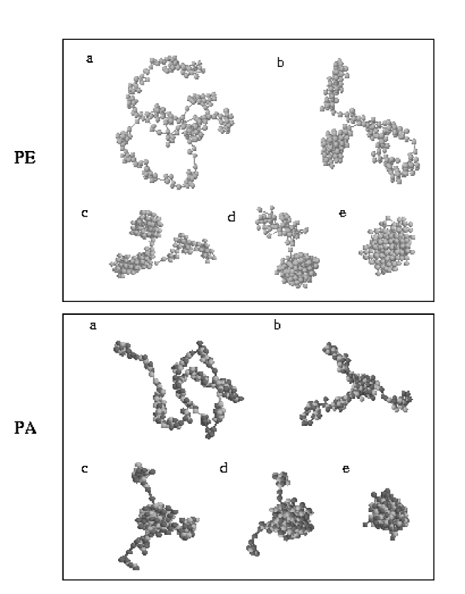
FIG. 1.: Snapshots of the conformations sampled in the dynamics of approach to the globular state starting from $\Theta$-solvent conditions. The final temperature is $l_{B}=5a_{o}$. For PA dark circles have $q=+e$ and grey circles have $q=-e$. The simulations are performed by integrating the Langevin equations. The details are given Ref.[4]. The top panel is for PE and the lower one is for PA; $N=240$ for both PE and PA; $v_{2}=-2.97a_{o}^{3}$ for PE $v_{2}=-6.18a_{o}^{3}$ for PA (the second virial coefficient $v_{2}$ gives an estimate of the quality of the solvent[4]). The counterions are explicitly included only in the simulation of PE. The solvent quality is such that the combined systems of the collapsed PE chain and the counterions form a Wigner Crystal[4]. The corresponding morphology of PA is clearly more disordered (compare structure ’e’ in the top and bottom panel).

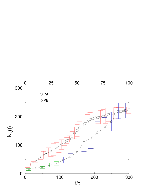
FIG. 2.: Time evolution of the number of particles belonging to the largest cluster $N_{S}(t)$ in a randomly charged single polyampholyte and a polyelectrolyte ($N=240$). The time scale for PA is given in the upper line. There are inherent numerical difficulties in computing $N_{s}(t)$ for finite sized systems. For a given trajectory there is not a sharp boundary for the largest cluster because of this the error-bars are large. Nevertheless, we observe linear increase of $N_{S}(t)$ for $t>100\tau$ (PE) and $t>30\tau$ for (PA) where $\tau=a_{o}^{2}/D$. This implies the Lifshitz-Slyozov growth mechanism i.e. $S(t)\sim N_{S}(t)^{1/3}\sim t^{1/3}$. At long times $N_{s}(t)$ saturates indicating the completion of globule formation.

REFERENCES

- [1] J.-L. Barrat and J.-F. Joanny, Adv. Chem. Phys. XCIV, 1 (1996).
- [2] V. A. Bloomfield, Biopolymers 31, 1471 (1991); V. A. Bloomfield, Curr. Opinion in Struc. Biol. 6, 334 (1996).
- [3] D. K. Treiber and J. R. Williamson, Curr. Opin. Struct. Biol. 9, 339 (1999).
- [4] N. Lee and D. Thirumalai, cond-mat 9907199 (1999).
- [5] U. Micka, C. Holm, K. Kremer, cond-mat 9812044 (1998).
- [6] F. J. Solis and M. Olvera de la Cruz, cond-mat 9908084 (1999).
- [7] M. Olvera de la Cruz, L. Belloni, M. Delsanti, J. P. Dalbiez, O. Spalla, M. Drifford, J. Chem. Phys. 103, 5781 (1995); P. Gonzalez-Mozuelos and M. Olvera de la Cruz J. Chem. Phys. 103, 3145 (1995).
- [8] H. Schiessel, P. Pincus, Macromolecules 31, 7953 (1998).
- [9] G. S. Manning, J. Chem. Phys. 51, 924 (1969).
- [10] E. Pitard and H. Orland, Europhys. Lett. 41, 467 (1998)
- [11] I.M. Lifshitz, and V. V. Slyozov, J. Phys. Chem. Solids 19, 35 (1961)).
- [12] E. Pitard, Europhys. J. B. 7, 665 (1999)
- [13] A. V. Dobrynin, M. Rubinstein, S. P. Obukhov, Macromolecules 29, 2974 (1996).
- [14] The mapping of PE with condensed counterions to PA rests on the assumption that the condensed counterions are relatively immobile on time scales . This is not expected to be strictly obeyed because because lateral motions (along the chain backbone) of counterions does occur. We justify this by explicit comparisons between theory and Langevin simulations. For PA the charge correlations are, by definition, given by Eq.(5).
- [15] For homopolymers it follows from [13] that where . This time scale may correspond to local cluster formation seen in computer simulations[16].
- [16] Y. A. Kuznetsov, E. G. Timoshenco and K. A. Dawson, J. Chem. Phys. 103, 4807 (1995); A. Byrne, P. Kiernan, D. Green and K. A. Dawson, J. Chem. Phys. 102, 573 (1995); G.E. Crooks, B. Ostrovsky, Y. Bar-Yam, cond-mat 9905393 (1999)).
- [17] P. G. de Gennes, J. Phys. (Paris) Lett. 46, L-639, (1985); A. Halperin, P. M. Goldbart, cond-mat 9905306 (1999).
- [18] Y. Kantor and M. Kardar, Europhys. Lett. 27, 643 (1994); Y. Kantor and M. Kardar, Phys. Rev. E 51, 1299 (1995).
- [19] For attractive interactions between like charged rods induced by correlations in counterions see B. -Y. Ha, Andrea J. Liu, Phys. Rev. Lett. 79, 1289 (1997); B. -Y. Ha, Andrea J. Liu, Phys. Rev. Lett. 81, 1011 (1998); N. Gnbech-Jensen, R. J. Mashl, R. F. Bruinsma, W. M. Gelbart, Phys. Rev. Lett. 78, 2477 (1997); R. Podgornik, V. A. Parsegian,Phys. Rev. Lett. 80, 1560 (1998).