State Space Reconstruction Parameters in the Analysis of Chaotic Time Series - the Role of the Time Window Length

Abstract

The most common state space reconstruction method in the analysis of chaotic time series is the Method of Delays (MOD). Many techniques have been suggested to estimate the parameters of MOD, i.e. the time delay $\tau$ and the embedding dimension $m$. We discuss the applicability of these techniques with a critical view as to their validity, and point out the necessity of determining the overall time window length, $\tau_{w}$, for successful embedding. Emphasis is put on the relation between $\tau_{w}$ and the dynamics of the underlying chaotic system, and we suggest to set $\tau_{w}\geq\tau_{p}$, the mean orbital period; $\tau_{p}$ is approximated from the oscillations of the time series. The procedure is assessed using the correlation dimension for both synthetic and real data. For clean synthetic data, values of $\tau_{w}$ larger than $\tau_{p}$ always give good results given enough data and thus $\tau_{p}$ can be considered as a lower limit ($\tau_{w}\geq\tau_{p}$). For noisy synthetic data and real data, an upper limit is reached for $\tau_{w}$ which approaches $\tau_{p}$ for increasing noise amplitude.

Key word index: time series, chaos, state space reconstruction, correlation dimension

1 Introduction

State space reconstruction is the first step in non-linear time series analysis of data from chaotic systems including estimation of invariants and prediction. For a recent review of these topics see [1] and [2]. Reconstruction consists of viewing a time series $x_{k}=x(k\tau_{s})$, $k=1,\ldots,N$ in a Euclidean space ${\mathbb{R}}^{m}$, where $m$ is the embedding dimension and $\tau_{s}$ is the sampling time. Doing this, we hope that the points in ${\mathbb{R}}^{m}$ form an attractor that preserves the topological properties of the original unknown attractor. A standard way to reconstruct the state space is the Method of Delays (MOD). Using MOD, each $m$-dimensional embedding vector is formed as $\mathbf{x}_{k}=[x_{k},x_{k+\rho},\ldots,x_{k+(m-1)\rho}]^{T}$ where $\rho$ is a multiple integer of $\tau_{s}$ so that the delay time $\tau$ equals $\rho\tau_{s}$ [3]. The $m$ coordinates of each point $\mathbf{x}_{k}$ are samples from the time series (separated by a fixed $\tau$) covering a time window of length $\tau_{w}=(m-1)\tau$ (or $\tau_{w}=(m-1)\rho$ as multiple of $\tau_{s}$).

The fundamental theorem of reconstruction, introduced first by Takens [4] and extended more recently in [6], gives no restriction on $\tau$ while for $m$ states the sufficient (but not necessary) condition $m\geq 2d+1$, where $d$ is the fractal dimension of the underlying attractor . Takens’ theorem is valid for the case of infinitely many noise-free data. In practice, however, with a limited number of possibly noisy observations, the selection of $\tau$ and $m$ is rather important for the quality of the reconstruction. Many methods have been suggested for estimating these parameters, but they are all empirical in nature and do not – as we show – necessarily provide appropriate estimates. This is a rather typical situation regarding state space reconstruction in general.

While there will always be uncertainties related to reconstruction from real data, it is still important to try to improve the procedures. We suggest $\tau_{w}$ as an independent parameter instead of focusing on the interrelated parameters $\tau$ and $m$ of MOD. The time window length is of particular importance since it determines, in a certain sense, the amount of information passed from the time series to the embedding vectors. For a given $\tau_{w}$, one may then select a sufficiently large $m$. Suggestions for the selection of $\tau_{w}$ have been made in [7], [8], [9], [10], [11] and [12] but to our knowledge there has been little systematic work regarding this parameter. We give procedures for estimating $\tau_{w}$ from the signal. Only time series from continuous systems are treated. For discrete systems, one typically sets $\rho=1$, reducing the number of parameters to one – the embedding dimension, since $\tau_{w}=m-1$.

The quality of the reconstructions is assessed using the correlation dimension [13]. The resulting reconstructions may not be the most suitable for other purposes such as estimation of Lyapunov exponents and prediction. However, with improved reconstructions for dimension estimation it is likely that the technique will be valuable also in other cases.

In section 2, we discuss several of the methods suggested up to now for estimating $\tau$ and $m$ in MOD and comment on the underlying ideas as well as on the validity of the results. In section 3, we establish the role of $\tau_{w}$ in reconstruction and give simple ways to estimate it. Finally, in section 4, the correlation dimension is used to assess the proposed procedure using noise-free and noise-corrupted synthetic data as well as real data.

2 Suggested methods for estimating the MOD-parameters

A very helpful approach in visualizing the reconstruction problem is to consider the reconstruction as an orthogonal projection from some high $p$-dimensional state space onto an $m$-dimensional subspace defined by the $m$ coordinates of the reconstructed vectors. Defining the linear mapping $B:{\mathbb{R}}^{p}\longrightarrow{\mathbb{R}}^{m}$, from each $p$-dimensional vector ${\mathbf{x}}_{k}^{p}$ to an $m$-dimensional vector ${\mathbf{x}}_{k}^{m}$, we have ${\mathbf{x}}_{k}^{m}=B{\mathbf{x}}_{k}^{p}$, where the rows of the $m\!\times\!p$ matrix $B$ are orthonormal. The $p$ coordinates of ${\mathbf{x}}_{k}^{p}$ are actually all the samples in the time window $\tau_{w}$ and in the case of MOD, where $p-1=\tau_{w}=(m-1)\rho$, the $m$ coordinates of the projected subspace are every $\rho$’th sample starting with the first, i.e. each row of $B$ has one 1 and $p-1$ zeros. Obviously, one can find other $m$-dimensional subspaces using a smaller $\rho$ (which may not cover the whole $\tau_{w}$). Using $\rho=1$ results in an unfavorable reconstruction if the time series is densely sampled because then the attractor lies on the diagonal in ${\mathbb{R}}^{m}$. (The successive samples differ very little from each other.) In such a projection we utilize only the $m$ first samples of $\tau_{w}$. Other projections may be considered such as the one employed in the Singular Spectrum Approach (SSA) [7]. This method yields first a transformation of the natural coordinate system to another orthogonal system, ranking the $p$ new directions according to the variance they explain, followed by a projection onto the $m$ first directions. The rows of the $B$ matrix are then the first $m$ eigenvectors of the $p\!\times\!p$ sample covariance matrix of the embedding vectors. The reconstruction viewed as a projection from the hyperspace determined by $\tau_{w}$ reveals the importance of this parameter. For MOD, the subspace is defined completely by the parameters $\tau$ (or $\rho$) and $m$ and for SSA by $p$ and $m$.

Certain statements supporting current methods for estimating $\tau$ and $m$ have been widely accepted and almost adopted as axioms. We do not intend to question all the existing methodology on MOD state space reconstruction, but feel that a discussion is needed regarding the guidelines used to choose the parameters.

2.1 Comments on the selection of the delay time

Consider first $\tau$ and the two following widely accepted criteria:

1. The reconstructed attractor must be expanded from the diagonal (implying that $\tau$ should not be too small) but not too much so that it folds back (implying that $\tau$ should not be too large).

2. The components of the vector $\mathbf{x}_{k}$ must be uncorrelated.

Note the similarity of the two criteria: increasing $\tau$ expands the attractor from the diagonal and the components get less correlated; beyond some range of $\tau$, folding may occur and the components again get correlated. These goals are intuitively reasonable for $m=2$, while the generalization to a larger $m$ is not always straightforward as we show below. Many methods based on geometric properties seek the $\tau$ that makes the attractor cover the largest region or expands it maximally from the diagonal [14], [12], [15]. However, the goal of stretching the attractor from the diagonal to get “good” reconstructions is based rather on empirical than theoretical grounds. In theory, a good reconstruction means near topological equivalence of the reconstructed attractor to the original one. One way to assess topological equivalence is to check whether stretching and folding are proportionally the same in the two attractors. In practice, this is done by checking whether the inter-distances of points remain proportionally the same in the two attractors or, alternatively, by checking whether nearby points on the original attractor remain relatively close on the reconstructed attractor. This last property is not always preserved when we expand the attractor from the diagonal, even for proper expansions according to the two above criteria. We show this for the Lorenz system [16] in Fig. 1.

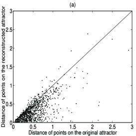
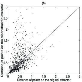
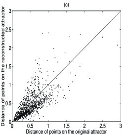
Figure 1: Correlation diagrams of the distances of points on the original attractor ($x$-axis) and on the reconstructed attractor ($y$-axis) for the Lorenz system. Results are shown for 10% of the 20000 data points sampled with $\tau_{s}=0.01$ time units. For each point on the original attractor the distance from its nearest neighbor is computed and keeping track of the time indices the distance of the corresponding points on the reconstructed attractor is then found. The attractor is reconstructed with MOD, $m=3$ and $\rho=1$ in (a), $\rho=18$ in (b), and $\rho=9$ in (c).

Fig. 1a shows that when $\tau$ is very small ($\tau=0.01$) the reconstructed attractor lies almost on the diagonal and the points are generally getting closer than the corresponding points on the original attractor. One expects that this problem is resolved when we expand the attractor sufficiently ($\tau=0.18$ which gives the minimum of the so-called mutual information – see below). But the opposite phenomenon is observed instead as shown in Fig. 1b, i.e. points that are close on the original attractor become more distant on the reconstructed attractor. Further, we show in Fig. 1c that the distances are more balanced for the reconstruction with a comparably small value of $\tau$ ($\tau=0.09$) which is not apparent from the two above criteria. The point we want to infer from this remark is that there is not necessarily a meaningful answer to the question: Why should we seek the $\tau$ that gives sufficient expansion from the diagonal? Expansion per se does not guarantee a configuration of the reconstructed attractor closer to the original one.

Concerning the second criterion, the estimates for $\tau$ are based either on linear decorrelation, choosing $\tau$ such that $R(\tau)=0$, where $R$ is the autocorrelation function, or general decorrelation choosing $\tau$ to be the first minimum of the mutual information $I(\tau)$ as developed in [18]. These two methods guarantee decorrelation (linear or general) between two successive components $x_{k}$ and $x_{k+\tau}$ of the reconstructed vector $\mathbf{x}_{k}$. But even if $x_{k}$ and $x_{k+\tau}$ are uncorrelated and $x_{k+\tau}$ and $x_{k+2\tau}$ are uncorrelated, it does not follow that $x_{k}$ and $x_{k+2\tau}$ are also uncorrelated. As an example, we show in Fig. 2 $R$ and $I$ for a time series from the Taylor-Couette experiment in the chaotic regime [19] which exhibits strong decorrelation for some lag $\tau$ and strong correlation for lag $2\tau$.

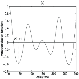
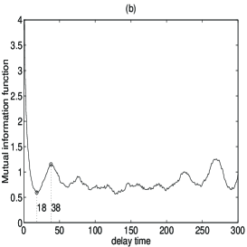
Figure 2: Autocorrelation function $R(\tau)$ in (a) and mutual information $I(\tau)$ in (b) for a time series of 10000 data measured from the Taylor-Couette experiment in the chaotic regime. Note the approximate matching of the zeros of $R$ to minimums of $I$ and the extremes of $R$ to maximums of $I$ indicating a dominant linear correlation. Moreover, note that the first decorrelation time is for $\rho\sim 20$ while for $\rho\sim 40$ there is maximum correlation.

We believe that the behavior of the correlation functions in Fig. 2 are often met in applications since chaotic time series from low dimensional systems frequently show pseudo-periodicities.

One may be confronted also with other problems attempting to estimate $\tau$: the autocorrelation function may get approximately zero only after an extremely long time, as for the $x$-variable of the Lorenz system, or the mutual information may not have a clear minimum, as is the case with the physiological data used below.

2.2 Comments on the selection of the embedding dimension

The standard way to find $m$ is to use some criterion which the geometry of the attractor must meet and check for which embedding dimension $m^{*}$ this is fulfilled as the attractor is embedded in successively higher dimensional spaces. Then $m^{*}$ is the lowest embedding dimension to be used for reconstruction. Obviously, in estimating $m$, $\tau$ is fixed when MOD is used.

Among different geometrical criteria (including also the correlation dimension), the most popular seems to be the method of “False Nearest Neighbors” (FNN) developed in [20] and enhanced recently in [21]. The rationale behind this method has also been discussed in [22] and [23]. This criterion concerns the fundamental condition of no self-intersections of the reconstructed attractor. The original attractor lies on a smooth manifold of dimension $\lceil d\rceil$. Self-intersections of the reconstructed attractor indicate that it does not lie on a smooth manifold and thus the reconstruction is not successful. The condition of no self-intersections states that if the attractor is to be reconstructed successfully in ${\mathbb{R}}^{m}$, then all neighbor points in ${\mathbb{R}}^{m}$ should also be neighbors in ${\mathbb{R}}^{m+1}$. The method checks the neighbors in successively higher embedding dimensions until it finds only a negligible number of false neighbors when increasing the dimension from $m^{*}$ to $m^{*}+1$. This $m^{*}$ is chosen as the lowest embedding dimension that gives reconstructions without self-intersections. However, the fact that the distances between neighboring points do not change when measured in ${\mathbb{R}}^{m}$ and in ${\mathbb{R}}^{m+1}$, does not necessarily mean that these points are also true neighbors on the original attractor.

Specifically, one has to consider the interdependence of $m$ and $\tau$. The estimation of $m$ depends on the selection of $\tau$ ($\rho$) as we show in Fig. 3 for the Lorenz system.

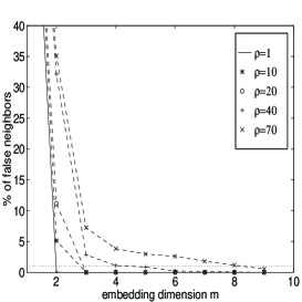
Figure 3: Plot of the percent of false neighbors detected as the embedding dimension is increased for different values of $\tau$. The algorithm of FNN has been implemented for a time series of 10000 samples of the $x$ variable of the Lorenz system. The different curves correspond to the time delays given in the legend as multiple of the sampling time $\tau_{s}=0.01$. The horizontal stippled line shows the 1% level of false neighbors which is often used as the discriminative threshold value.

The proportion of false nearest neighbors does not fall to zero for the same $m$ as $\tau$ increases but rather the estimated $m$ increases slowly with $\tau$. Thus, the estimation of $m$ is somewhat arbitrary unless the method finds the same $m$ for a sufficiently large range of $\tau$ values. For a very small $\tau$, there is a typical underestimation of $m$. Such a $\tau$ forces the attractor to lie near the diagonal in ${\mathbb{R}}^{m}$. Increasing $m$ by one has little effect on the geometry of the attractor as it will still lie near the diagonal of ${\mathbb{R}}^{m+1}$. All the points will apparently look as true neighbors leading to a wrong conclusion.

The method is very sensitive to noise giving larger values of $m$ for noisy data as pointed in [23] and [24]. In fact, the effect of noise is greater for larger values of $\tau$. This is a serious drawback of the method because in real applications we are led to choose a larger $m$ than we really need. This problem is particularly relevant for MOD, where the projections are chosen without regard to noise filtering which is partly accomplished using SSA-reconstructions [9].

Another method that has been suggested to estimate $m$ is based on truncating the singular spectrum of SSA (for details see [7] and [25]). In fact, the idea behind this linear approach is, given the hyperspace of dimension $p$, to find the smallest subspace (hyperplane) that approximately bounds the attractor. This subspace is spanned by the eigenvectors corresponding to the largest eigenvalues of the sample covariance matrix, i.e. the directions where the attractor has the largest variance. However, a strange attractor lies on a manifold which occupies all directions in the embedded space (very much like noise) and a clear cut-off is not expected [26]. On the other hand, if this approach is implemented locally it can reveal the dimension of the tangent space to the manifold and the averaging over a grid of local regions can give a robust estimate of $m$ as shown in [27]. However, this estimate depends on the choice of the dimension $p$ of the hyperspace, i.e. the time window length $\tau_{w}$.

From these remarks we conclude that many of the existing methods for estimating $\tau$ and $m$ are based on somewhat arbitrary criteria and do not always guarantee good reconstructions. The performance depends on the problem at hand.

3 The time window length - $\tau_{w}$

When analysing a time series one typically begins with an initial reconstruction, and implements a non-linear method to this and other modified reconstructions until a stable result is attained. Here we concentrate on the time window length $\tau_{w}$ to determine the reconstruction.

There is probably no uniquely best way to choose an initial $\tau_{w}$. We will argue that it may be reasonable to set $\tau_{w}$ equal to the “memory” of the system, i.e. the measurement record needed to determine future observations as reliably as possible. For practical reasons, one would like the shortest possible $\tau_{w}$. Geometrically, one could associate such a $\tau_{w}$ with the mean orbital period $\tau_{p}$, i.e. the mean time between two consecutive visits to a local neighborhood. For low-dimensional chaotic systems showing pseudo-periodicity, the mean orbital period could naturally be associated with the mean time between visiting a Poincare section.

For several chaotic systems, $\tau_{p}$ carries significant information about the dynamics. For systems that generate attractors with a sheet-like structure in ${\mathbb{R}}^{3}$ (see for example [28]), it can be shown that the Poincare section gives points that in a scatter plot lie approximately on a curve, which is the one dimensional manifold that embeds an attractor very much like the strange attractor of the logistic map. The same result may be obtained by selecting the points from the extremes or maxima of the time series directly instead of using reconstruction and Poincare section. This has been shown for the Lorenz system [29] and the Rössler system [30]. We found similar results studying the oscillations of other systems with sheet-like structure, such as the Rabinovich-Fabrikant system [31] and the Mackey Glass system for $\Delta=17$ [32] (for details of this system see below).

As indicated above, the procedure suggested here requires only an initial estimate of $\tau_{w}$ which is subsequently adjusted. Given only a set of observations, a very simple solution is to select the initial $\tau_{w}$ as the mean time between peaks (tbp) of the original time series. In general, tbp will be less than $\tau_{p}$, and thus it is natural to consider tbp a lower limit. For a low dimensional system, e.g. defined asymptotically in ${\mathbb{R}}^{3}$, it is reasonable to assume that an orbital period corresponds to an oscillation when projected down to the observed axis, and thus $\tau_{p}=tbp$. For more complicated systems in higher dimensional spaces, a complete orbit may form more than one oscillation. In that case, $\tau_{p}$ should be estimated as the average over a pattern of oscillations.

The equation of Mackey Glass [32]

$$\dot{x}=\frac{0.2x(t-\Delta)}{1+[x(t-\Delta)]^{10}}+0.1x(t)$$ (1)

is a good example to show how one can find lower limits for $\tau_{w}$ from the oscillations of the time series. This time delay differential equation was discretized following the iterative scheme in [33], and segments of the time series for different $\Delta$ are shown in Fig.4 with solid grey lines.

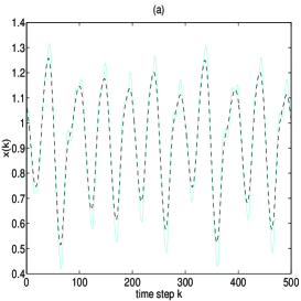
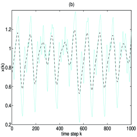
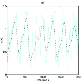
Figure 4: The solid grey lines in all three figures are for segments of the Mackey Glass time series for different $\Delta$ and the stippled lines after smoothing with a $k$-FIR filter. (a) $\Delta=17$, $\tau_{s}=1$, and $k=10$. (b) $\Delta=30$, $\tau_{s}=1$, and $k=30$. (c) $\Delta=100$, $\tau_{s}=1$, and $k=80$.

For $\Delta=17$, the attractor is low dimensional ($d\simeq 2$ [13]) and an orbital period can be assumed to correspond to a single oscillation (solid grey line in Fig. 4a). Then $\tau_{p}$ can be easily estimated as $tbp$ after filtering the time series to avoid close peaks that do not correspond to distinct oscillations (stippled black line in Fig. 4a), and thus for $\Delta=17$ we can conclude that $\tau_{w}\geq\tau_{p}=tbp\simeq 50$ time units.

For $\Delta=30$, the attractor has a higher dimension ($d\simeq 3$ [13]) and as Fig. 4b shows, in many parts of the time series there are systematic variations over a pattern of oscillations (often comprised of a small and a large oscillation), approximately repeating itself. Filtering gives a new time series with one peak for each such pattern, facilitating the computation of $\tau_{p}$ from the $tbp$ of the filtered time series giving $\tau_{w}\geq\tau_{p}\simeq 100$.

For $\Delta=100$ in Fig. 4c, the attractor is much more complicated ($d\simeq 7.1$ [33]) and therefore it is difficult to observe patterns of oscillations that repeat themselves (but not as difficult as to make Poincare sections). However, in some particular parts of the time series, consecutive similar patterns may be observed showing implicit correspondence to orbital periods (see Fig. 4c). Hard filtering allows us even to assign a peak to each pattern giving $\tau_{w}\geq\tau_{p}\simeq 330$. Note that filtering is performed only in order to discern the representative peaks, especially for higher dimensional systems. Noisy time series should be filtered anyway, before estimating $\tau_{p}$ to avoid the fake peaks that are due to noise.

Up to this point we have assumed that the measurement function is well defined according to Takens’ generic assumptions, so that the oscillations in the observed time series do reflect the periodic-like orbits of the original system and vice versa. However, this is not always the case and as an example of a “good” and “bad” mapping let us consider the $x$ and $z$ variable of the Rössler system [34] (see Fig. 5).

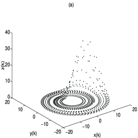
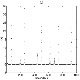
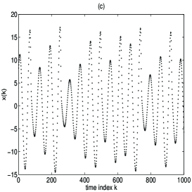
Figure 5: (a) A trajectory of the Rössler system in ${\mathbb{R}}^{3}$. (b) Measurements of the $z$ variable of the trajectory. (c) Measurements of the $x$ variable of the trajectory. Note that the oscillations of the time series in (b) do not reveal all orbital periods associated with the trajectory while in (c) they do.

In the time series of the $x$ variable, the oscillations represent the real orbits while in the time series of the $z$ variable the orbital periods can hardly be recognized. In the latter case, an analysis will fail to identify the correct attributes of the system unless a very large amount of data is provided to compensate for the bad mapping. We found, for example, that for measurements over the same epoch, the correlation dimension of the Rössler attractor was well estimated by the $x$-measurements but significantly underestimated by the $z$-measurements due to the “knee” phenomenon we discuss below.

We here suggest working directly in the time domain to estimate $\tau_{w}$ instead of considering periods corresponding to dominant frequencies as suggested by [7] and [10]. Chaotic data will in general not show well defined frequency peaks. Other suggestions regarding $\tau_{w}$ have been presented in the literature [8], [11] and [12]. Some attempted to estimate $\tau_{w}$ based on decorrelation criteria from the autocorrelation function and the mutual information [9], [35] and [36]. In one paper treating this issue, [9], lower and upper limits for $\tau_{w}$ where based on the autocorrelation function and it was proposed to set $\tau_{c}\leq\tau_{w}\leq 4\tau_{c}$, where $\tau_{c}$ is the correlation time defined as the delay where the autocorrelation function is $1/e$. This lower limit is much smaller than $\tau_{p}$ for most systems. An upper limit for $\tau_{w}$ was given in [11] by $2\sqrt{\frac{3\langle x^{(0)}\rangle}{\langle x^{(1)}\rangle}}$, where $\langle x^{(0)}\rangle$ and $\langle x^{(1)}\rangle$ are the mean values of the time series and its first derivative, respectively. We found that for many systems this upper limit is also smaller than $\tau_{p}$.

4 Correlation dimension and $\tau_{w}$

We now discuss the use of $\tau_{w}$ in the time series analysis. A natural procedure is to start with an initial $\tau_{w}$ and perform calculations – in this case computing the correlation dimension $\nu$ – for a sufficiently large $m$. Then $\tau_{w}$ is modified, the calculations repeated, and so on. To be able to conclude that a valid result has been obtained, reasonably stable values have to be found over a range of $\tau_{w}$ values.

First we define the correlation integral $C(r)$, a statistic that measures the fraction of points on the attractor being less than $r$ units apart

$$C(r)=\frac{1}{N(N-1)}\sum_{i,j=1,|i-j|>K}^{N}\Theta(r-||\mathbf{x}_{i}-\mathbf{x}_{j}||)$$ (2)

where $\Theta(x)$ is the Heaviside function, defined as $\Theta(x)=1$ for $x\geq 0$ and $\Theta(x)=0$ for $x<0$, and $K$ is used to omit time-correlated points in the computation of $C(r)$. The Euclidean norm is used because it gives more robust results in the presence of noise [37]. For deterministic systems, the correlation integral scales as $C(r)\sim r^{\nu}$, where theoretically $r\rightarrow 0$. Preferably, $\nu$ should be estimated from the slope of the graph of $\log C(r)$ against $\log r$ over a sufficient range $[r_{1},r_{2}]$ of small interdistances. However, due to noise or to limited data, an approximately constant slope may be maintained only for larger values of $r_{1}$ and $r_{2}$. We chose $r_{2}/r_{1}=4$ for the length of the interval, and searched over all such intervals to find the one where the computed $\nu$ varied least. The mean value of the slope in this interval is the estimated $\nu$, and it is always reported together with the standard deviation (shown with bars in the following figures).

A key observation is that the estimate of the correlation dimension of a chaotic time series (clean or noisy) is approximately the same under variations of the parameters $\rho$ and $m$ while keeping $\tau_{w}=(m-1)\rho$ fixed (assuming that $m$ is always larger than the dimension of the attractor). Only few workers seem to have thought along these lines ([8], [9], [10] and [12]). The typical features are demonstrated in Fig. 6 which shows the correlation dimension estimates for different $\tau_{w}$ for clean and noisy data from the Lorenz system.

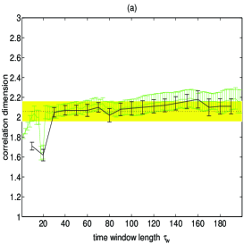
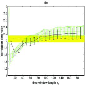
Figure 6: Plot of the correlation dimension estimate $\nu$ for MOD reconstruction with different $\tau_{w}$ for time series of the $x$ variable of the Lorenz system. The bars denote the standard deviation of the estimate. In each figure the grey curve with grey error bars correspond to $\rho=2$ while the black ones to $\rho=10$. In (a) the estimation is based on the clean time series of 4000 data sampled with $\tau_{s}=0.02$ and in (b) on the same data but corrupted with $5\%$ noise. The horizontal stippled line shows the correct plateau for $\nu=2.06$ and the shaded area the confidence interval of $\pm 5\%$ of the correct $\nu$.

Note how the grey and black curves match for the clean data in Fig. 6a. They correspond to the same $\tau_{w}$ but with $\rho=2$ and $\rho=10$, respectively. Once $\tau_{w}$, and thus the $p$-dimensional hyperspace, has been determined, the particular projection chosen is not critical as long as the projection is sufficient, i.e. $m>\nu$ and $\rho\simeq\frac{p-1}{m-1}\equiv\frac{\tau_{w}}{m-1}$. This is so, because the interdistances of points remain statistically the same in ${\mathbb{R}}^{p}$ and in ${\mathbb{R}}^{m}$. Considering all the coordinates or only the selected subset has the same effect on the computation of the interdistance as long as a suitable norm is used, e.g. the Euclidean norm [37].

When white noise is added to the clean Lorenz data (Fig. 6b) the two curves still match but now show an increasing trend with $\tau_{w}$. The estimation of $\nu$ is more sensitive to the choice of $\tau_{w}$ in the presence of noise.

Results for the estimation of $\nu$ from noisy data or few data (compared to the minimum number of data required) should be interpreted with caution because they are derived from scaling properties based on large $r$. For smaller $r$, the scaling is corrupted by noise or distorted due to few neighbors in state space. In the case of attractors with different scaling properties for small and large $r$ (a phenomenon referred to as a “knee” [38]), erronous estimates are obtained from the scaling for large $r$ when noise or insufficient data length mask the correct scaling for small $r$. Such a phenomenon is observed for the $z$-measurements of the Rössler system mentioned before. The correct scaling ($\nu\simeq 2.01$) can be only detected for very small inter-point distances $r$ requiring a very large number of data, otherwise another scaling is detected for larger $r$, underestimating $\nu$.

The estimation of $\nu$, even when it is constrained only to large $r$, is not straightforward as it varies with $\tau_{w}$ and a typical situation is shown in Fig. 7 for Lorenz system.

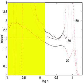
Figure 7: Plot of the slope of the graph $\log C(r)$ against $\log r$ for the time series of 4000 data from the Lorenz system, sampled with $\tau_{s}=0.02$ and with $5\%$ additive noise. The three curves are derived from reconstructions with $\rho=10$ and $m=3$ (minimum embedding dimension), $m=9$ and $m=17$ and are identified by the length of $\tau_{w}$ marked on the figure. The scaling interval of least variation is denoted with the black solid line segment for each slope curve. The grey area shows roughly the region where inter-point distances are corrupted by noise leaving a small interval of $r$ to estimate $\nu$ and making the choice of $\tau_{w}$ critical. The horizontal stippled line shows the correct plateau for $\nu\simeq 2.06$.

Too small $\tau_{w}$ ($\tau_{w}=20$) or too large $\tau_{w}$ ($\tau_{w}=160$) gives uncertain and wrong estimates while for $\tau_{w}$ larger than but still close to $\tau_{p}=50$ (here $\tau_{w}=80$) the scaling is clear indicating a reliable estimate. On the other hand, the range of suitable $\tau_{w}$ depends on the length of the time series; the longer the time series, the broader the limits for $\tau_{w}$. Noise also restricts $\tau_{w}$ from above because the slope curves derived for increasing $\tau_{w}$ do not saturate. Setting a criterion for the acceptance of the $\nu$-estimate, e.g. $\pm 5\%$ of the correct value, an upper limit $\tau_{n}$ for the range of $\tau_{w}$ may be found which varies with the amplitude of the noise (e.g. $\tau_{n}\simeq 110$ for Fig. 6b). It is thus expected that the scaling gets distorted as $\tau_{w}$ icreases over $\tau_{n}$ giving less confident estimates as shown with the slope curve for $\tau_{w}=160$ in Fig. 7. So, when the time series is corrupted with noise, the $\nu$-estimates are more biased and the interval $[\tau_{p},\tau_{n}]$ of the accepted $\tau_{w}$ shrinks from above, and it may be no reliable estimate of $\nu$ for any $\tau_{w}$ if the impact of noise is so large that $\tau_{n}$ decreases to the level of $\tau_{p}$.

Thus when estimating $\nu$ from a limited number of noisy data we seek the range of $\tau_{w}$ that gives clear scaling for large $r$ keeping in mind that the results are still ambiguous due to the possible different scaling for small and inaccessible $r$ (the “knee” phenomenon). In the sequel, we consider in more detail simulated data corrupted with noise as well as real data.

4.1 Noisy synthetic data

Most of the time series we use here have length $N=4000$ adjusting the sampling time $\tau_{s}$ accordingly in order to have enough oscillations as well as enough samples for each oscillation. It follows that the number of data points is not the best measure of the record length. We therefore also quote the number of $\tau_{p}$ within the record, denoted $\#\tau_{p}$, together with the number of samples in $\tau_{p}$. Note that under changes of the reconstruction parameters or the noise amplitudes, the values $r_{1}$ and $r_{2}$ of the scaling interval $[r_{1},r_{2}]$ that gives $\nu$-estimates with least variance may change as well.

Results for the time series from the $x$-variable of the Lorenz system with $\tau_{s}=0.02$ and $\tau_{p}\simeq 50$ and $\#\tau_{p}\simeq 80$ were shown in Fig. 6. For the clean data, legitimate estimates of $\nu$ (within $\pm 5\%$ of the correct $\nu=2.06$ shown as a shaded zone in the figure) were obtained for a large interval of $\tau_{w}$ values beginning even lower than $\tau_{p}$. As $\tau_{w}$ is increased long beyond $\tau_{p}$ the estimates increase somewhat and have larger variance. When $5\%$ white Gaussian noise is added to these data, the correlation dimension is underestimated significantly for $\tau_{w}<\tau_{p}$, and for $\tau_{w}>\tau_{n}\simeq 110$, $\nu$ is overestimated with larger variance.

The attractor derived from the $x$-variable of the Rössler system has a simpler structure than the Lorenz attractor and about the same dimension. However, estimates of $\nu$ are more dependent on the reconstruction parameters and the amplitude of the noise. The time series is sampled with $\tau_{s}=0.1$ that gives $60$ samples in each oscillation and about $66$ oscillations, which are comparable to the $\tau_{p}$ and $\#\tau_{p}$ for the Lorenz data. In Fig. 8, the $\nu$-estimates are plotted against

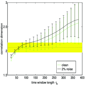
Figure 8: Plot of the correlation dimension estimate $\nu$ for MOD reconstruction with different $\tau_{w}$ for time series of the $x$ variable of the Rössler system. The grey curve with grey error bars correspond to the clean data and the black to the same data corrupted with $2\%$ noise. Here, $N=4000$, $\tau_{s}=0.1$ and $\rho=20$. The horizontal stippled line shows the correct plateau for $\nu=2.01$ and the shaded area the confidence interval of $\pm 5\%$ of the correct $\nu$.

$\tau_{w}$ for the clean and noisy Rössler data displayed with grey and black error bars respectively, together with the $\pm 5\%$-zone of the accepted range of $\nu$. Here, as well as in the following estimations, we keep $\rho$ fixed ($\rho=20$ in Fig. 8) and vary $m$. This is done for convenience since the results are essentially the same for other combinations of $\rho$ and $m$ (refer back to Fig. 6). For the clean data, reasonable and confident $\nu$-estimates can be found for a small range of $\tau_{p}=60\leq\tau_{w}<140$ (the grey error bars in the $\pm 5\%$-zone in the figure). When just $2\%$ white noise is added to these data, the small horizontal plateau seems to disappear (the black line in Fig. 8) and only $\nu$-estimates close to $\tau_{p}$ and above can be accepted, which is in accordance with the proposed $\tau_{w}$.

The Mackey Glass attractor for $\Delta=17$ has the same dimensionality as the two last attractors but gives less biased estimates of $\nu$. For $\tau_{s}=1$, we found $\tau_{p}=50$ and $\#\tau_{p}\simeq 80$ from single oscillations. In Fig. 9, results from the estimation of $\nu$

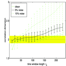
Figure 9: Plot of the correlation dimension estimate $\nu$ for MOD reconstruction with different $\tau_{w}$ for time series of the Mackey Glass equation for $\Delta=17$. The solid grey curve with solid grey error bars correspond to the clean data, the solid black to the noisy data with $5\%$ noise and the stippled grey to the noisy data with $10\%$ noise. Here, $N=4000$, $\tau_{s}=1$ and $\rho=12$. The horizontal stippled line shows the correct plateau for $\nu=2$ and the shaded area the confidence interval of $\pm 5\%$ of the correct $\nu$.

are presented in the same way as for the Rössler data. For the clean data, a very reliable $\nu$-estimate is derived over a large interval of $\tau_{w}$, $[20,160]$ (from the $\pm 5\%$-criterion). When $5\%$ noise is added, confident estimates are obtained only close to $\tau_{p}$, and when $10\%$ noise is added, reasonable estimates are only obtained for $\tau_{w}\simeq\tau_{p}$.

When $\Delta=30$, the dimension of the attractor increases to $\nu\simeq 3$ [13]. However, using $N=4000$ and $\tau_{s}=2$ an underestimate ($\nu\simeq 2.5$) was found. For this $\tau_{s}$, the $\tau_{p}$ estimated with the mean time for patterns of two oscillations (cf. section 3) is kept down to $\tau_{p}=50$ and $\#\tau_{p}\simeq 80$, as for $\Delta=17$. The results from estimation of $\nu$ for clean and noisy data with $5\%$ and $10\%$ noise (shown in Fig. 10a)

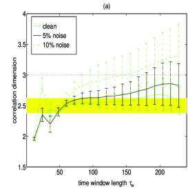
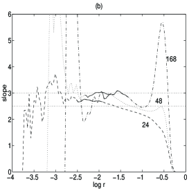
Figure 10: (a) Plot of the correlation dimension estimate $\nu$ for MOD reconstruction with different $\tau_{w}$ for time series of the Mackey Glass equation for $\Delta=30$. The solid grey curve with solid grey error bars correspond to the clean data, the solid black to the noisy data with $5\%$ noise and the stippled grey to the noisy data with $10\%$ noise. Here, $N=4000$, $\tau_{s}=2$ and $\rho=12$. The horizontal stippled line shows the correct plateau for $\nu\simeq 3.0$ and the shaded area the confidence interval of $\pm 5\%$ of the underestimated $\nu\simeq 2.5$. (b) Plot of the slope of the graph $\log C(r)$ against $\log r$ for the same type of data but for $N=30000$. The three curves are derived from reconstructions with $\rho=12$ and $m=3$, $m=6$ and $m=17$ and are identified by the length of $\tau_{w}$ marked on the figure. The scaling interval of least variation is denoted with the black solid line segment for each slope curve. The two horizontal stippled lines show the two scalings of this attractor.

assert the use of $\tau_{p}$ as a lower limit for $\tau_{w}$ and the decrease of the interval of accepted values for $\tau_{w}$ from above and towards $\tau_{p}$ as the amplitude of the added noise is increased. The underestimation of $\nu$ is due to the limited number of data. This attractor shows a “knee” structure, i.e. it has also another scaling (the correct $\nu\simeq 3.0$) for small $r$ which can be detected only when many data are accumulated as shown in Fig. 10b. The slope for too small $\tau_{w}$ ($\tau_{w}=24$) underestimates $\nu$ while for $\tau_{w}\geq\tau_{p}$ the correct scaling is achieved (shown with the two curves for $\tau_{w}=48$ and $\tau_{w}=168$ in the figure). Note that these curves form a second scaling for larger $r$.

For $\Delta=100$, the Mackey Glass attractor gets high dimensional with $\nu\simeq 7$ [33]. Our results show a slightly lower $\nu$ with as few as $N=4000$. We sampled the discretized system with $\tau_{s}=10$ in order to have enough, but not too many, samples within the estimated mean orbital period, $\tau_{p}\simeq 33$, giving as many as $\#\tau_{p}\simeq 120$ repititions of the oscillation pattern that is assumed to correspond to an orbit of the underlying system. We deliberately keep the data record down to $N=4000$ in order to test our procedure for short time series (compared to the high dimensionality of the system). The estimated $\nu$ is an increasing function of $\tau_{w}$ both in values and uncertainty, showing some stability in value and in variance for $\tau_{p}\simeq 30\leq\tau_{w}\leq 45$. This is, however, an underestimation of $\nu$, possibly due to insufficient data (see Fig. 11).

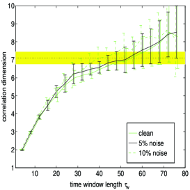
Figure 11: Plot of the correlation dimension estimate $\nu$ for MOD reconstruction with different $\tau_{w}$ for time series of the Mackey Glass equation for $\Delta=100$. The solid grey curve with solid grey error bars correspond to the clean data, the solid black to the noisy data with $5\%$ noise and the stippled grey to the noisy data with $10\%$ noise. Here, $N=4000$, $\tau_{s}=10$ and $\rho=4$. The horizontal stippled line shows the correct plateau for $\nu\simeq 7.1$ and the shaded area the confidence interval of $\pm 5\%$ of the correct $\nu$.

Adding $5\%$ noise does not alter the $\nu$-estimates but just increases moderately the uncertainty of the estimates; when $10\%$ noise is added, the $\nu$-estimates for $\tau_{w}>\tau_{p}$ vary significantly from those of the clean data.

These findings, as well as results for the Rabinovich-Fabrikant system [31], and the four-dimensional Rössler Hyperchaos system [39], not shown here, confirm our suggestion for estimating $\tau_{w}$ with $\tau_{p}$ giving the best estimates of $\nu$. If the effect of noise or limited length of the time series is such that estimation of $\nu$ can be made only for a short range of $\tau_{w}$ values, this is close to and little larger than $\tau_{p}$.

4.2 Real data

In addition to simulated data, observations from physical controlled experiments on low dimensional deterministic processes should be used to assess the validity of non-linear methods. The noise level is often insignificant in such cases. Here we use a time series of $N=4000$ samples from the Taylor Couette experiment in the chaotic regime. We estimated $\tau_{p}\simeq 75$ and $\#\tau_{p}\simeq 54$, but the results for the estimation of $\nu$ do not change for longer time records covering more oscillations (increasing either $N$ or $\tau_{s}$ if we insist on keeping $N$ small). Contrary to most of the previous results from simulated data with noise, the estimated $\nu$ varies little with $\tau_{w}$ as shown in Fig. 12.

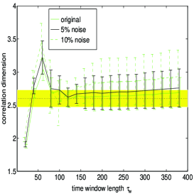
Figure 12: Plot of the correlation dimension estimate $\nu$ for MOD reconstruction with different $\tau_{w}$ for time series from the Taylor Couette experiment in the chaotic regime. The solid grey curve with solid grey error bars correspond to the original data, the solid black to the original data corrupted with $5\%$ noise and the stippled grey to the original data corrupted with $10\%$ noise. Here, $\rho=20$ is chosen for reconstructions varying with $m$. The horizontal stippled line shows the correct plateau for $\nu\simeq 2.6$ and the shaded area the confidence interval of $\pm 5\%$ of the correct $\nu$.

For all $\tau_{w}>\tau_{p}$ the etsimates are more or less fixed to $\nu\simeq 2.6$, approximately the value given in the literature [19], with a slowly increasing uncertainty for $\tau_{w}>150$. This indicates that there is little noise in the data and the dimension of the chaotic attractor can be identified even with large $\tau_{w}$ (up to $2\tau_{p}$), so that the choice of $\tau_{w}$ is not critical. However, when we add noise to these data, to simulate a larger experimental uncertainty, the estimates have as expected a larger variance, but for $\tau_{w}$ close to $\tau_{p}$ the estimates are the same as for the original time series. For larger $\tau_{w}$ there is a systematic overestimation of $\nu$, showing again that the optimal $\tau_{w}$ for correct estimation is close to $\tau_{p}$.

We now turn to observational data that are not output of a controlled experiment, and concentrate on physiological data of the Electroencephalogram (fig13) from epileptic patients (e.g. see [40]). Dimension estimation of physiological data has been a hot subject the last years. However, the results to date are not promising, partly because different procedures are often used giving different $\nu$-estimates for the same type of data, and partly because these data do not seem to share the same nice chaotic properties as the well-studied simulated data [41]. Previous work on $\nu$-estimation of EEG epileptic signals reported low dimensional attractors of varying dimension between 2 and 6, according to the physiological nature of the data, the data acquisition process, the computational scheme of estimation, as well as the parameter setting for reconstruction ([42], [43], [44] and [45]).

Here, we use a short time series from an epileptic seizure of $N=3400$ data sampled with $\tau_{s}=0.005sec$. The oscillations of the time series evolve irregularly, so the estimated $tbp\simeq 30$ does not seem to be directly related to $\tau_{p}$. With a more thorough examination of the sequence of oscillations, we can distinguish patterns of oscillations that may correspond to orbital periods of the potential underlying attractor. In Fig. 13a we show

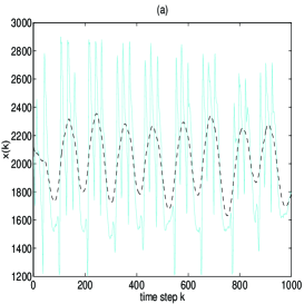
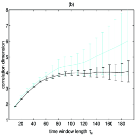
Figure 13: (a) Segment of the EEG time series of an epileptic seizure sampled with $\tau_{s}=0.005sec$ (solid grey line) and after smoothing with a 40 point FIR filter (stippled black line). (b) Plot of the correlation dimension estimate $\nu$ for MOD reconstruction with different $\tau_{w}$ for EEG time series in epileptic seizure. The grey curve with grey error bars correspond to estimation over a scaling interval $[r_{1},r_{2}]$ with $r_{2}/r_{1}=4$ while the black curve with black error bars correspond to $r_{2}/r_{1}=2$. The other parameters are $N=3400$, $\tau_{s}=0.005$ and $\rho=10$.

a part of the time series where such patterns are apparent. After severe filtering, the time corresponding to each pattern can be estimated by the tbp for the filtered time series giving $\tau_{p}\simeq 110$. Other parts of the time series are not so regular but still patterns of about the same time length can be identified qualitatively. The standard estimation procedure applied to these data gave no clear saturation of the $\nu$-estimate for increasing $\tau_{w}$, (grey curve in Fig. 13b). The estimate increases with increasing variance showing some flatness for a small region of values of $\tau_{w}$ around $100$. In fact, for $\tau_{w}>100$ there is scaling but over a shorter interval of interdistances $[r1,r2]$ not satisfying the more stringent criterion $r2/r1=4$. Relaxing this to $r2/r1=2$, which has previously been used for EEG signals [46], a clear saturation with $\nu\simeq 4$ is established for $\tau_{w}>100$, though with increasing variance (Fig. 13b). Thus, the optimal choice of $\tau_{w}$ for the computation of $\nu$ should be around $100$, which is close to $\tau_{p}=110$, the estimate of $\tau_{w}$ from the oscillations of the time series. Note that these results are not general for epileptic EEG signals. Other EEG data showed very poor scaling and no saturation for increasing $\tau_{w}$ even for $r2/r1=2$ [47] giving no valid estimate for $\nu$. In these cases, no patterns of oscillations could be observed.

5 Conclusions

Our analysis in section 2 showed that when one reconstructs with MOD, effective techniques for determining the delay time $\tau$ and the lowest embedding dimension $m$ are lacking. Concerning $\tau$, there is no standard indication of which value is the most appropriate. In fact, if we allow $m$ to be very large, we can even use a very small $\tau$ in the reconstruction. It seems that instead of relying on estimates for $\tau$ (such as the zero of the autocorrelation function or the minimum of mutual information) and $m$ (such as the estimate from false nearest neighbors) one could rather employ “trial and error”. In fact, this seems to be common in practice.

A more systematic and less tedious way to make reconstructions has been proposed here focusing on the time window length $\tau_{w}$. We argued that $\tau_{w}$ is the first parameter to be determined when reconstructing the state space and suggested that it should be approximated by the mean orbital period $\tau_{p}$. For low dimensional attractors, $\tau_{p}$ is set to the time between peaks $tbp$, easily calculated by averaging the time between successive maxima of the time series. Noisy time series may be filtered before determining tbp. For higher dimensional and more complicated systems, the mean orbital period may be found from coherent patterns of oscillations. Computationally, this can be done measuring the “period” of such oscillating patterns, or applying strict filtering so that each pattern becomes one oscillation, and then compute the $tbp$.

With the estimation of $\tau_{w}$ and a sufficiently large $m$, the reconstruction is completely defined and can be used for further analysis of the time series. Regarding the correlation dimension, an initial estimate may be derived with $\tau_{w}=\tau_{p}$, and then checking whether the same estimate is obtained when $\tau_{w}$ is increased. For noisy data, the estimate remains the same only for $\tau_{w}$ close to $\tau_{p}$, as noise sets an upper limit to $\tau_{w}$. The proposed parameter setting turned out to give the most confident $\nu$-estimates for all data analyzed where estimation was possible.

References

- [1] Kugiumtzis, D. and Lillekjendlie, B. and Christophersen, N., “Chaotic Time Series Part I: Estimation of Some Invariant Properties in State Space”, Modeling, Identification and Control, 15, 205 – 224, 1994.
- [2] Lillekjendlie, B. and Kugiumtzis, D. and Christophersen, N., “Chaotic Time Series Part II: System Identification and Prediction”, Modeling, Identification and Control, 15, 225 – 243, 1994.
- [3] Packard, N. H. and Crutchfield, J. P. and Farmer, J. D. and Shaw, R. S., “Geometry from a Time Series”, Physical Review Letters, 45, 712, 1980.
- [4] Takens, F., “Detecting Strange Attractors in Turbulence”, Dynamical Systems and Turbulence, Warwick 1980, Lecture Notes in Mathematics 898, editors Rand, D. A. and Young, L. -S., Springer, Berlin, 366 – 381, 1981.
- [5] Mañé, R., “On the Dimensions of the Compact Invariant Sets of Certain Non-linear Maps”, Dynamical Systems and Turbulence, Warwick 1980, Lecture Notes in Mathematics 898, editors Rand, D. A. and Young, L. -S., Springer, Berlin, 230 – 242, 1981.
- [6] Sauer, T. and Yorke, J. A. and Casdagli, M., “Embedology”, Journal of Statistical Physics, 65, 579 – 616, 1991.
- [7] Broomhead, D. S. and King, G. P., “Extracting Qualitative Dynamics from Experimental Data”, Physica D, 20, 217 – 236, 1986.
- [8] Caputo, J. G. and Malraison, B. and Atten, P., “Determination of Attractor Dimension and Entropy for Various Flows: An Experimentalist’s ViewPoint” Dimensions and Entropies in Chaotic Systems, editor Mayer-Kress, G., Springer-Verlag, Berlin, 180 – 190, 1986.
- [9] Albano, A. M. and Muench, J. and Schwartz, C. and Mees, A. I. and Rapp, P. E., “Singular Value Decomposition and the Grassberger-Procaccia Algorithm”, Physical Review A, 38, 3017 – 3026, 1988.
- [10] Grassberger, P. and Schreiber, T. and Schaffrath, C., “Non-linear time sequence analysis”, International Journal of Bifurcation and Chaos, 1, 521 – 547, 1991.
- [11] Gibson, J. F. and Farmer, J. D. and Casdagli, M. and Eubank, S., “An Analytic Approach to Practical State Space Reconstruction”, Physica D, 57, 1 – 30, 1992.
- [12] Rosenstein, M. T. and Collins, J. J. and De Luca, C. J., “Reconstruction Expansion as a Geometry-based Framework for Choosing Proper Delay Times”, Physica D, 73, 82 – 98, 1994.
- [13] Grassberger, P. and Procaccia, I., “Measuring the Strangeness of Strange Attractors”, Physica D, 9, 189 – 208, 1983.
- [14] Buzug, T. and Pfister, G., “Comparison of Algorithms Calculating Optimal Embedding Parameters for Delay Time Coordinates”, Physica D, 58, 127 – 137, 1992.
- [15] Kember, G. and Fowler, A. C., “A Correlation Function for Choosing Time Delays in Phase Portrait Reconstructions”, Physics Letters A, 179, 72 – 80, 1993.
- [16] Lorenz, E. N., “Deterministic Nonperiodic Flow”, J. Atmos. Sci., 20, 130, 1963.
- [17] Tsonis, A. A., Chaos: From Theory to Applications, Plenum Press, New York, 1992.
- [18] Fraser, A. M. and Swinney, H., “Independent Coordinates for Strange Attractors from Mutual Information”, Physical Review A, 33, 1134 – 1140, 1986.
- [19] Brandstater, A. and Swinney, H., “Strange Attractors in Weakly Turbulent Couette-Taylor Flow”, Physical Review A, 35, 2207 – 2220, 1987.
- [20] Kennel, M. B. and Brown, R. and Abarbanel, H. D. I., “Determining Embedding Dimension for Phase-Space Reconstruction Using a Geometrical Construction”, Physical Review A, 45, 3403 – 3411, 1992.
- [21] Kennel, M. B. and Abarbanel, H. D. I., “False Neighbors and False Strands: A Reliable Minimum Embedding Dimension Algorithm”, Preprint, 1995.
- [22] Liebert, W. and Pawelzik, K. and Schuster, H. G., “Optimal Embeddings of Chaotic Attractors from Topological Considerations”, Europhysics Letters, 14, 521 – 526, 1991.
- [23] Aleksić, Z., “Estimating the Embedding Dimension”, Physica D, 52, 362 – 368, 1991.
- [24] Abarbanel, H. D. I. and Brown, R. and Sidorowich, J. J. and Tsimring, L. S., “Analysis of Observed Chaotic Data in Physical Systems”, Reviews of Modern Physics, 65, 1331 – 1392, 1993.
- [25] Vautard, R. and Yiou, P. and Ghil, M., “Singular-spectrum Analysis: A Toolkit for Short, Noisy Chaotic Signals”, Physica D, 58, 95 – 126, 1992.
- [26] Mees, A. I. and Rapp, P. E. and Jennings, L. S., “Singular-value Decomposition and Embedding Dimension”, Physical Review A, 36, 340 – 346, 1987.
- [27] Passamante, A. and Hediger, T. and Gollub, M., “Fractal Dimension and Local Intrinsic Dimension”, Physical Review A, 39, 3640 – 3645, 1989.
- [28] Medio, A., Chaotic Dynamics: Theory and Applications to Economics, Cambridge University Press, Cambridge, 1992.
- [29] Ott, E., Chaos in Dynamical Systems, Cambridge University Press, Cambridge, 1993.
- [30] Olsen, L. F. and Degn, H., “Chaos in Biological Systems”, Guarterly Reviews of Biophysics, 18, 165 – 225, 1985.
- [31] Rabinovich, M. I. and Fabrikant, A. L., “Stochastic Self-modulation of Waves in Nonequilibrium Media”, Sov. Phys. JETP, 50, 311, 1979.
- [32] Mackey, M. and Glass, L., “Oscillation and chaos in physological control systems”, Science, 197, 287, 1977.
- [33] Ding, M. and Grebogi, C. and Ott, E. and Sauer, T. and Yorke, J. A., “Estimating Correlation Dimension from a Chaotic Time Series: when does a Plateau Onset Occur?”, Physica D, 69, 404 – 424, 1993.
- [34] Rössler, O. E., “An Equation for Continuous Chaos”, Physics Letters A, 57, 397 – 398, 1976.
- [35] Albano, A. M. and Passamante, A. and Farell, M-E., “Using Higher-Order Correlations to Define an Embedding Window”, Physica D, 54, 85 – 97, 1991.
- [36] Martinerie, J. M. and Albano, A. M. and Mees, I. A. and Rapp, P. E., “Mutual Information, Strange Attractors, and the Optimal Estimation of Dimension”, Physical Review A,45, 7058 – 7064, 1992.
- [37] Kugiumtzis, D, “Assessing Different Norms in Nonlinear Analysis of Noisy Time Series”, Preprint, 1996.
- [38] Theiler, J., “Estimating Fractal Dimension”, J. Opt. Soc. Am. A, 7, 1055 – 071, 1990.
- [39] Rössler, O. E., “An Equation for Hyperchaos”, Physics Letters A, 71, 155 – 157, 1979.
- [40] Jansen, B. H., “Quantitative Analysis of Electroencephalograms: is There Chaos in the Future?”, International Journal of Biomedical Computing, 27, 95 – 123, 1991.
- [41] Kantz, H. and Schreiber, T., “Dimension Estimates and Physiological Data”, Chaos, 5, 143 – 154, 1995.
- [42] Rapp, P. E. and Zimmerman, I. D. and Albano, A. M. and Deguzman, G. C. and Greenbaum, N. N., “Dynamics of Spontaneous Neural Activity in the Simian Motor Cortex: the Dimension of Chaotic Neurons”, Physics Letters A, 110, 335 – 338, 1985.
- [43] Babloyantz, A. and Destexhe, A., “Low-dimensional Chaos in an Instance of Epilepsy”, Proceedings of the National Academy of Sciences of the United States of America, 83, 3513 – 3517, 1986.
- [44] Frank, G. W. and Lookman, T. and Nerenberg, M. A. H. and Essex, C. and Lemieux, J. and Blume, W, “Chaotic Time Series Analyses of Epileptic Seizures”, Physica D, 46, 427 – 438, 1990.
- [45] Pijn, J. P. and Neerven, J. V. and Noest, A. and Lopes da Silva, F. H., “Chaos or Noise in EEG Signals; Dependence on State and Brain Site”, Electroencephalography and Clinical Neurophysiology, 79, 371 – 381, 1991.
- [46] Pritchard, D. W. and Duke, W. S., “Measuring Chaos in the Brain: A Tutorial Review of Nonlinear Dynamical EEG Analysis”, Intern J. Neuroscience, 67, 31 – 80, 1992.
- [47] Madsen, H, Non-linear Methods for the Analysis of Electroencephalograms (EEG), Department of Informatics, Oslo, 186 pp (in Norwegian), 1995.