BU-CCS-960101 Integer Lattice Gases

Abstract

We generalize the hydrodynamic lattice gas model to include arbitrary numbers of particles moving in each lattice direction. For this generalization we derive the equilibrium distribution function and the hydrodynamic equations, including the equation of state and the prefactor of the inertial term that arises from the breaking of galilean invariance in these models. We show that this prefactor can be set to unity in the generalized model, therby effectively restoring galilean invariance. Moreover, we derive an expression for the kinematic viscosity, and show that it tends to decrease with the maximum number of particles allowed in each direction, so that higher Reynolds numbers may be achieved. Finally, we derive expressions for the statistical noise and the Boltzmann entropy of these models.

I Lattice Gases

Lattice gas automata (LGA) are a class of dynamical systems in which particles move on a lattice in discrete time steps. If the collisions between the particles conserve mass and momentum, the coarse-grained behavior of the system can be shown to be that of a viscous fluid in the appropriate scaling limit [1, 2, 3, 4]. Used as an algorithm for simulating hydrodynamics, the method has the virtues of exact conservation laws, and of unconditional numerical stability.

In a typical LGA, there is an association between the lattice vectors and the particles at each site. If there are $n$ lattice vectors, then the state of the site is represented by $n$ bits. Each bit represents the presence or absence of a particle in the corresponding direction. At each time step, a particle propagates along its corresponding lattice vector and then collides with other arriving particles at the new site. The collisions are required to conserve particle mass and momentum.

Relevant dimensionless quantities of a LGA are the Knudsen number, Kn, defined as the ratio of the mean-free path to the characteristic length scale; the Strouhal number, Sh, defined as the ratio of the mean-free time to the characteristic time scale; the Mach number, M, defined as the ratio of the characteristic velocity to the speed of sound; the Reynolds number, $\mbox{Re}\sim\mbox{M}/\mbox{Kn}$; and the fractional variation of density from its average value, $\delta\rho/\rho$. Hydrodynamic behavior [5] is attained in the limit as Kn and Sh go to zero. Viscous hydrodynamics [5] is attained when $\mbox{Sh}\sim\mbox{Kn}^{2}$ in this limit. Incompressible viscous hydrodynamics [6] is then attained when we also have $\mbox{M}\sim\mbox{Kn}$ so that $\mbox{Re}\sim{\cal O}(1)$, and $\delta\rho/\rho\sim\mbox{Kn}^{2}$.

The Chapman-Enskog procedure is a perturbation expansion in the above-described asymptotic ordering. For a LGA whose collisions conserve mass and momentum on a lattice of sufficient symmetry (quantified below), the local equilibrium distribution function can be shown to be Fermi-Dirac in nature [2, 3, 4]. The Chapman-Enskog procedure can then be used to compute the correction to this Fermi-Dirac distribution and thereby show [1, 2, 3, 4] that the pressure, $P$, and the momentum density, ${\bf u}$, obey the following equations in the asymptotic limit:

$\displaystyle\mbox{\boldmath$\nabla$}\cdot{\bf u}=0$

$\displaystyle\frac{\partial{\bf u}}{\partial t}+\frac{g(\rho)}{\rho}{\bf u}\cdot\mbox{\boldmath$\nabla$}{\bf u}=-\mbox{\boldmath$\nabla$}P+\nu(\rho)\nabla^{2}{\bf u},$

where $\rho$ is the fluid density (a constant in this limit). The analysis also yields expressions for the functions $g(\rho)$ and $\nu(\rho)$, and an equation of state for $P$. In particular, the form of these equations, the equation of state, and the expression for the function $g(\rho)$ depend only on the fact that mass and momentum are conserved – and are the only things conserved – by the collisions. The expression for the viscosity, $\nu(\rho)$ depends on the details of the collision rules used.

Since the fluid density $\rho$ is a constant in the asymptotic limit, the factors $g(\rho)$ and $\nu(\rho)$ are also constants. As has been noted, the latter is the fluid viscosity. The presence of the former is reflective of a breaking of galilean invariance, due to the fact that the lattice itself constitutes a preferred galilean frame of reference. For a single-phase LGA, the former factor can easily be scaled away by redefining the momentum density and pressure as

$\displaystyle{\bf U}\equiv g(\rho){\bf u}$

and

$\displaystyle{\cal P}\equiv g(\rho)P,$

where ${\bf u}$ and $P$ are those measured in the simulation. For compressible flow, or for multiphase flow with interfaces, however, the presence of the $g(\rho)$ factor is problematic, and various techniques have been proposed to remove it. It has been shown that this can be done by judiciously violating semi-detailed balance in the collision rule [7], or by adding many rest particles at each site [8].

The unconditional stability of the lattice gas procedure arises from a requirement that the collisions satisfy a statistical reversibility condition known as semi-detailed balance (SDB). The collision process is fully specified by the transition matrix $A(s\rightarrow s^{\prime})$ which is the probability that the incoming state $s$ will result in outgoing state $s^{\prime}$. Since collisions must result in some outgoing state, conservation of probability requires that

$$\sum_{s^{\prime}}A(s\rightarrow s^{\prime})=1.$$ (I.1)

SDB is then the condition that

$$\sum_{s}A(s\rightarrow s^{\prime})=1.$$ (I.2)

(Note that the condition of detailed balance (DB), $A(s\rightarrow s^{\prime})=A(s^{\prime}\rightarrow s)$, implies that of SDB, but not vice versa; that is, SDB is a weaker condition than DB.) From SDB, it is possible to prove an $H$-theorem, from which follows the unconditional stability of the lattice gas algorithm.

An important limitation of the lattice gas procedure has to do with the statistical noise associated with the coarse-grained averaging that is necessary to get the hydrodynamic quantities that obey the above fluid equations. For $n$ bits per site, and for coarse-grained averages over blocks of $N$ sites, the noise is of order $\sim 1/\sqrt{nN}$. For some applications – most notably the simulation of complex fluids – a certain controllable amount of noise is actually desirable because it is essential to the physics; for simple fluid dynamics computations, on the other hand, the noise is a nuisance.

II Lattice Boltzmann Equations

Because of their noise and lack of galilean invariance, LGA have been replaced by Lattice Boltzmann Equations (LBE) for many hydrodynamics applications of interest in recent years [9]. These methods keep track only of an averaged occupation number of particles in each direction at each site. Moreover, the collision operator most often used is a simple relaxation to a noiseless equilibrium, thereby eliminating the statistical fluctuations that are inherent in the LGA method. This means that in complex fluid applications for which statistical fluctuations are an essential part of the physics, they have to be reintroduced artificially [10].

For a lattice Boltzmann equation corresponding to a lattice gas with only one bit per lattice vector, this real-valued distribution function is bounded between zero and one. This need not be the case, however, and the LBE procedure allows one to tailor the equilibrium distribution function to satisfy certain desiderata. Among these is the ability to demand galilean invariance ($g(\rho)=1$) [11].

At the same time, the LBE method gives up two of the principal advantages of LGA’s: Due to the roundoff error inherent in manipulations of real numbers on a computer, it no longer maintains the conservation laws exactly. Moreover, LBE’s are no longer unconditionally stable; indeed, they are subject to a variety of numerical instabilities, most of which are not well understood.

III Integer Lattice Gas Automata

In this paper, we investigate a simple generalization of the lattice gas concept that can be used to control the level of statistical fluctuations – reducing it if desired, but not necessarily eliminating it altogether – while maintaining the conservation laws exactly, preserving unconditional stability, and allowing for galilean invariance.

The use of a single bit per each of $n$ directions to represent the state of a given lattice site means that the number of particles moving along any lattice direction is either zero or one. We generalize this by allowing for up to $L$ bits per direction, for a total of $nL$ bits per site, so that the number of particles moving along any lattice direction can range from $0$ to $2^{L}-1$. The total number of states per site is then $2^{nL}$. Computationally, this means that the state of each direction is described by an integer of $L$ bits; hence, the terminology, Integer Lattice Gas Automata (ILGA).

To simplify the derivation of the hydrodynamic equations of an ILGA, we use the Boltzmann molecular chaos approximation, so that all quantities in our analysis are ensemble averaged, and we indiscriminately commute the application of this average with the collision process. We also assume that the particles are of unit mass. Denote the ensemble-averaged value of the $\ell$th bit in the $i$th direction by $N^{i,\ell}$, where $0<i<n-1$ and $0<\ell<L-1$. Also, denote the lattice vector for the $i$th direction by ${\bf c}_{i}$. The distribution function for the total number of particles in each direction is then,

$$N^{i}=\sum_{\ell=0}^{L-1}2^{\ell}N^{i,\ell}.$$ (III.3)

The ensemble-averaged mass and momentum densities are then given by

$$\rho=\sum_{i=0}^{n-1}N^{i}=\sum_{i=0}^{n-1}\sum_{\ell=0}^{L-1}2^{\ell}N^{i,\ell}$$ (III.4)

and

$${\bf u}=\sum_{i=0}^{n-1}{\bf c}_{i}N^{i}=\sum_{i=0}^{n-1}\sum_{\ell=0}^{L-1}2^{\ell}{\bf c}_{i}N^{i,\ell}.$$ (III.5)

Let us also associate an energy $\varepsilon_{i}$ with each particle in direction $i$. The ensemble-averaged energy density is then given by

$$\varepsilon=\sum_{i=0}^{n-1}\varepsilon_{i}N^{i}=\sum_{i=0}^{n-1}\sum_{\ell=0}^{L-1}2^{\ell}\varepsilon_{i}N^{i,\ell}.$$ (III.6)

IV Thermodynamics of the Integer Lattice Gas

We first consider the thermodynamics of the integer lattice gas. The grand canonical partition function is

$\displaystyle{\cal Z}=\sum_{\{N\}}\exp\left[-\beta\left(E-\mbox{\boldmath$\alpha$}\cdot{\bf P}-\mu M\right)\right],$

where the sum is over all possible states of the ILGA (that is, each $N^{i}({\bf x})$ is summed from $0$ to $2^{L}-1$), where $\beta$, $\alpha$ and $\mu$ are Lagrange multipliers, and where

$\displaystyle M\equiv\sum_{\bf x}^{V}\sum_{i}^{n}N^{i}({\bf x}),$

$\displaystyle{\bf P}\equiv\sum_{\bf x}^{V}\sum_{i}^{n}N^{i}({\bf x}){\bf c}_{i}$

and

$\displaystyle E\equiv\sum_{\bf x}^{V}\sum_{i}^{n}N^{i}({\bf x})\varepsilon_{i}$

are the total mass, momentum and energy, respectively, of all the particles on a lattice of $V$ sites. Thus, we have

$${\cal Z} = \sum_{\{N\}}\exp\left[-\beta\sum_{\bf x}^{V}\sum_{i}^{n}\left(\varepsilon_{i}-\mbox{\boldmath$\alpha$}\cdot{\bf c}_{i}-\mu\right)N^{i}({\bf x})\right]$$

$$= \sum_{\{N\}}\prod_{\bf x}^{V}\prod_{i}^{n}\exp\left[-\beta\left(\varepsilon_{i}-\mbox{\boldmath$\alpha$}\cdot{\bf c}_{i}-\mu\right)N^{i}({\bf x})\right]$$

$$= \prod_{\bf x}^{V}\prod_{i}^{n}\sum_{k=0}^{2^{L}-1}\exp\left[-\beta\left(\varepsilon_{i}-\mbox{\boldmath$\alpha$}\cdot{\bf c}_{i}-\mu\right)k\right]=\prod_{\bf x}^{V}\prod_{i}^{n}\sum_{k=0}^{2^{L}-1}(z^{i})^{k}$$

$$= \prod_{\bf x}^{V}\prod_{i}^{n}\left(\frac{1-(z^{i})^{2^{L}}}{1-z^{i}}\right)=\left[\prod_{i}^{n}\left(\frac{1-(z^{i})^{2^{L}}}{1-z^{i}}\right)\right]^{V},$$

where we have defined the fugacity

$$z^{i}\equiv\exp\left[-\beta\left(\varepsilon_{i}-\mbox{\boldmath$\alpha$}\cdot{\bf c}_{i}-\mu\right)\right].$$ (IV.7)

The grand potential is then

$\displaystyle\Omega=-\frac{1}{\beta}\ln{\cal Z}=-\frac{V}{\beta}\sum_{i}^{n}\ln\left(\frac{1-(z^{i})^{2^{L}}}{1-z^{i}}\right),$

so that

$\displaystyle\frac{\partial}{\partial\beta}\left(\beta\Omega\right)=-\frac{\partial}{\partial\beta}\ln{\cal Z}=V\sum_{i}^{n}\left(\frac{z^{i}}{1-z^{i}}-\frac{2^{L}(z^{i})^{2^{L}}}{1-(z^{i})^{2^{L}}}\right)\left(\varepsilon_{i}-\mbox{\boldmath$\alpha$}\cdot{\bf c}_{i}-\mu\right).$

We identify the equilibrium distribution function

$$F_{L}(z)\equiv\frac{z}{1-z}-\frac{2^{L}(z)^{2^{L}}}{1-(z)^{2^{L}}},$$ (IV.8)

which gives the mean number of particles moving in each lattice direction. Since this has a maximum of $2^{L}-1$, we also define the fractional occupation number

$\displaystyle f_{L}(z)\equiv\frac{F_{L}(z)}{2^{L}-1}.$

Figure 1 shows $f_{L}(z)$ plotted against $z$ for several values of $L$.

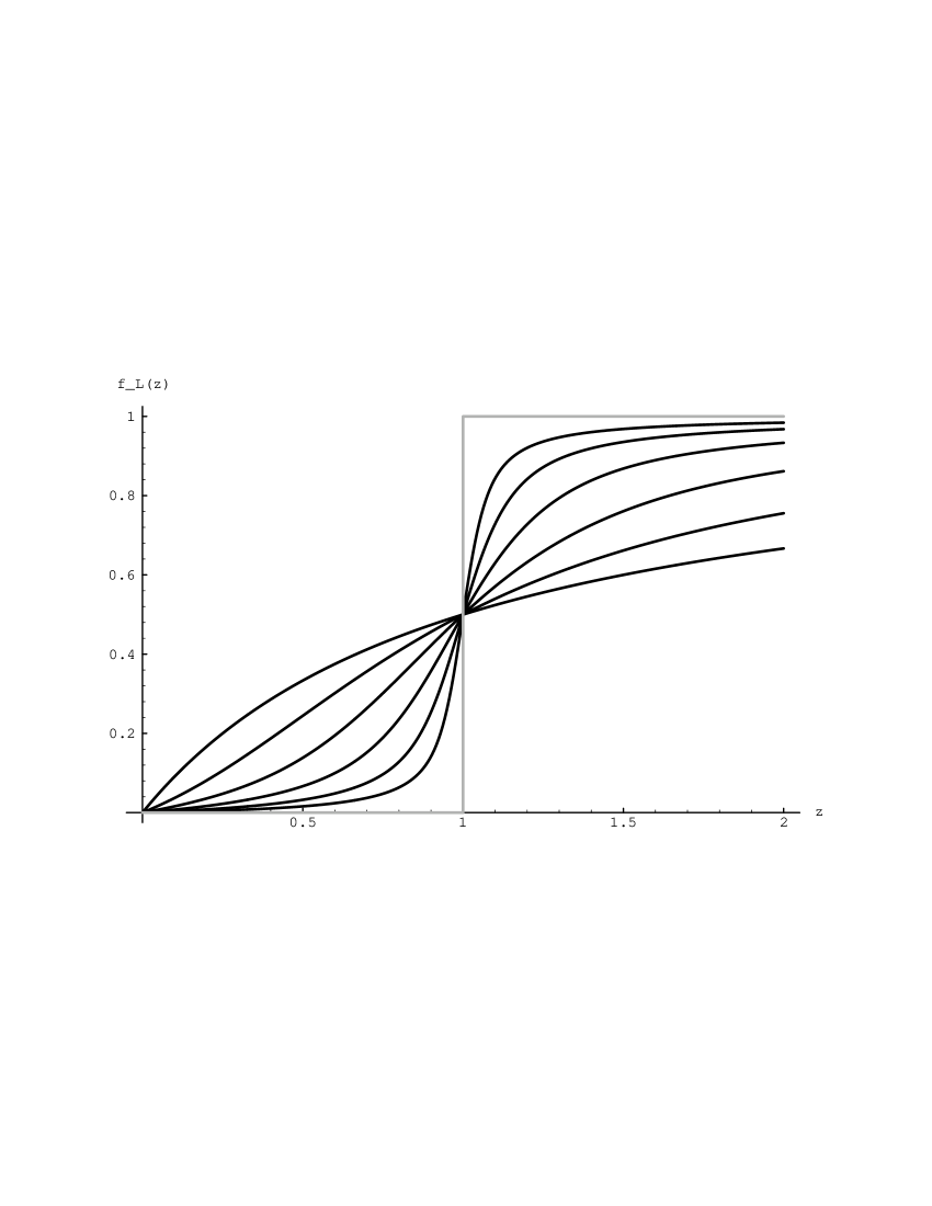
FIG. 1.: $f_{L}(z)$ versus $z$ for several values of $L$. The black curves represent $L$ values from 1 to 6, with increasing steepness, while the gray curve is the limit as $L\rightarrow\infty$.

In terms of the equilibrium distribution function, we have

$\displaystyle\Omega+\beta\frac{\partial\Omega}{\partial\beta}=\Omega-T\frac{\partial\Omega}{\partial T}=V\sum_{i}^{n}F_{L}(z^{i})\left(\varepsilon_{i}-\mbox{\boldmath$\alpha$}\cdot{\bf c}_{i}-\mu\right),$

where $T\equiv 1/\beta$ is the temperature. It follows that

$\displaystyle\Omega=\langle H\rangle-\mbox{\boldmath$\alpha$}\cdot\langle{\bf P}\rangle-\mu\langle M\rangle-T\langle S\rangle,$

where we have identified the average energy

$\displaystyle\langle H\rangle\equiv V\sum_{i}^{n}F_{L}(z^{i})\varepsilon_{i},$

the average momentum

$\displaystyle\langle{\bf P}\rangle\equiv V\sum_{i}^{n}F_{L}(z^{i}){\bf c}_{i},$

the average mass

$\displaystyle\langle M\rangle\equiv V\sum_{i}^{n}F_{L}(z^{i}),$

and the average entropy

$\displaystyle\langle S\rangle\equiv-\frac{\partial\Omega}{\partial T}=V\sum_{i}^{n}S_{L}(z^{i}).$

In the expression for the entropy we have defined the function

$$S_{L}(z)\equiv\ln\left(1-z^{2^{L}}\right)+\left(\frac{z^{2^{L}}}{1-z^{2^{L}}}\right)\ln\left(z^{2^{L}}\right)-\ln\left(1-z\right)-\left(\frac{z}{1-z}\right)\ln\left(z\right)$$ (IV.9)

as the entropy per lattice direction. Thus, in addition to the form for the equilibrium distribution function, this analysis has provided us with an expression for the entropy that is additive in the contributions from each lattice direction. In fact, it is straightforward to show that $S_{L}\rightarrow L\ln 2$ in the limit of large $L$, corresponding to a dominant contribution of $\ln 2$ per bit of state. The excess

$$\Delta S_{L}\equiv S_{L}-L\ln 2$$ (IV.10)

is then ${\cal O}(1)$ in $L$ and is plotted against the fractional occupation number $f_{L}(z)$ in Fig. 2. This can be interpreted as indicating that the bits are most random at half filling; elsewhere, the entropy is lower than $L\ln 2$ per bit.

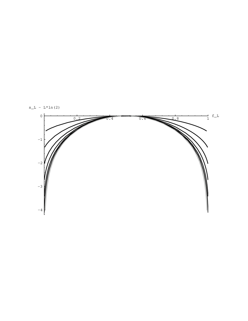
FIG. 2.: Entropy excess $\Delta S_{L}$ versus fractional occupation number $f_{L}(z)$. The black curves decrease with increasing $L$, and the gray curve is the limit as $L\rightarrow\infty$.

V Kinetic-Theoretical Treatment

As an alternative to the preceding thermodynamic treatment of the integer lattice gas, we can derive the principal results from a kinetic-theoretical argument. For example, to derive the form of the equilibrium distribution function, Eq. (IV.8), we can note that the equilibrium distribution function for each bit must still be Fermi-Dirac in form, since each individual bit is either occupied or not. Thus,

$\displaystyle N_{0}^{i,\ell}=\frac{1}{1+\exp\left[2^{\ell}\beta\left(\varepsilon_{i}-\mbox{\boldmath$\alpha$}\cdot{\bf c}_{i}-\mu\right)\right]},$

where the multipliers $\beta$, $\alpha$ and $\mu$ are determined in terms of the mass, momentum and energy densities by their definitions, Eqs. (III.4), (III.5) and (III.6). In terms of the fugacity, Eq. (IV.7), the above may be written,

$$N_{0}^{i,\ell}=\frac{1}{1+(z^{i})^{-2^{\ell}}}.$$ (V.11)

The equilibrium distribution function for each direction is then given by Eqs. (III.3) and (V.11),

$\displaystyle N_{0}^{i}=\sum_{\ell=0}^{L-1}2^{\ell}N_{0}^{i,\ell}=F_{L}(z^{i}),$

where we have defined the function

$$F_{L}(z)\equiv\sum_{\ell=0}^{L-1}\frac{2^{\ell}}{1+z^{-2^{\ell}}}.$$ (V.12)

In Appendix A we show that this sum is equal to the closed form derived in the previous section,

$$F_{L}(z)=\frac{z}{1-z}-\frac{2^{L}z^{2^{L}}}{1-z^{2^{L}}}.$$ (V.13)

VI Form of the Hydrodynamic Equations

To derive the hydrodynamic equations, we first expand the equilibrium distribution function in the Mach number. Here and henceforth, we specialize to the case of no internal energy, so that $\varepsilon_{i}=0$, and we can absorb the multiplier $\beta$ into $\alpha$ and $\mu$. Treating $\alpha$ as a small quantity, the fugacity can be written

$\displaystyle z^{i}=e^{\mu}\left(1+\mbox{\boldmath$\alpha$}\cdot{\bf c}_{i}+\frac{1}{2}\mbox{\boldmath$\alpha$}\mbox{\boldmath$\alpha$}:{\bf c}_{i}{\bf c}_{i}\right)=z_{0}+z_{1}^{i}+z_{2}^{i},$

where the subscripts of

$$z_{0} \equiv e^{\mu}$$

$$z_{1}^{i} \equiv z_{0}\mbox{\boldmath$\alpha$}\cdot{\bf c}_{i}$$

$$z_{2}^{i} \equiv \frac{z_{0}}{2}\mbox{\boldmath$\alpha$}\mbox{\boldmath$\alpha$}:{\bf c}_{i}{\bf c}_{i}$$

denote the order of the Mach number expansion, and we note that $z_{0}$ is independent of the direction $i$. It follows that

$\displaystyle N^{i}_{0}=F_{L}(z^{i})=F_{L}(z_{0}+z_{1}^{i}+z_{2}^{i}).$

Taylor expanding, we get

$\displaystyle N^{i}_{0}=F_{L}(z_{0})+z_{0}F_{L}^{\prime}(z_{0})\mbox{\boldmath$\alpha$}\cdot{\bf c}_{i}+\frac{1}{2}z_{0}\left[z_{0}F_{L}^{\prime}(z_{0})\right]^{\prime}\mbox{\boldmath$\alpha$}\mbox{\boldmath$\alpha$}:{\bf c}_{i}{\bf c}_{i}.$

To proceed, we must make some assumptions about the symmetries of the lattice. We demand that

$$\sum_{i=0}^{n-1}\bigotimes^{k}{\bf c}_{i}=A_{k}{\bf 1}_{k}$$ (VI.14)

for $0\leq k\leq 4$, where $\otimes$ denotes the outer product, and where ${\bf 1}_{k}$ is the completely symmetric and isotropic tensor of rank $k$,

$\displaystyle{\bf 1}_{0}=1$

$\displaystyle({\bf 1}_{1})_{i}=0$

$\displaystyle({\bf 1}_{2})_{ij}=\delta_{ij}$

$\displaystyle({\bf 1}_{3})_{ijk}=0$

$\displaystyle({\bf 1}_{4})_{ijkl}=\delta_{ij}\delta_{kl}+\delta_{ik}\delta_{jl}+\delta_{il}\delta_{jk}.$

Note that Eq. (VI.14) defines the coefficients $A_{k}$ for a given lattice.

We now demand that

$\displaystyle\rho=\sum_{i=0}^{n-1}N^{i}_{0}=A_{0}F_{L}(z_{0})+\frac{A_{2}\beta^{2}}{2}z_{0}\left[z_{0}F_{L}^{\prime}(z_{0})\right]^{\prime},$

and

$\displaystyle{\bf u}=\sum_{i=0}^{n-1}{\bf c}_{i}N^{i}_{0}=A_{2}z_{0}F_{L}^{\prime}(z_{0})\mbox{\boldmath$\alpha$}.$

If we now let $z$ denote the solution to the equation

$$\frac{\rho}{A_{0}}=F_{L}(z),$$ (VI.15)

it follows that the difference between $z$ and $z_{0}$ is of second order in the Mach number, so that we can solve for $\mu$ and $\alpha$. We find that

$\displaystyle\mbox{\boldmath$\alpha$}=\frac{{\bf u}}{A_{2}zF_{L}^{\prime}(z)},$

and that $\mu=\ln z_{0}$ where $z_{0}$ is the solution to the equation

$\displaystyle F_{L}(z_{0})=\frac{\rho}{A_{0}}-\frac{z\left[zF_{L}^{\prime}(z)\right]^{\prime}}{2A_{0}A_{2}\left[zF_{L}^{\prime}(z)\right]^{2}}u^{2}.$

Inserting these results into the distribution function, we find

$$N^{i}_{0}=\frac{\rho}{A_{0}}+\frac{{\bf u}\cdot{\bf c}_{i}}{A_{2}}+\frac{z\left[zF_{L}^{\prime}(z)\right]^{\prime}}{2A_{2}^{2}\left[zF_{L}^{\prime}(z)\right]^{2}}\left({\bf c}_{i}{\bf c}_{i}-\frac{A_{2}}{A_{0}}{\bf 1}_{2}\right):{\bf u}{\bf u},$$ (VI.16)

where, again, $z$ is defined by $F_{L}(z)=\rho/A_{0}$.

The inviscid part of the stress tensor is then given by

$$\sum_{i=0}^{n}{\bf c}_{i}{\bf c}_{i}N^{i}_{0} = \frac{A_{2}}{A_{0}}\rho+\frac{z\left[zF_{L}^{\prime}(z)\right]^{\prime}}{2A_{2}\left[zF_{L}^{\prime}(z)\right]^{2}}\left(\frac{A_{4}}{A_{2}}{\bf 1}_{4}-\frac{A_{2}}{A_{0}}{\bf 1}_{2}\otimes{\bf 1}_{2}\right):{\bf u}{\bf u}$$

$$= \left[\frac{A_{2}}{A_{0}}\rho+\frac{z\left[zF_{L}^{\prime}(z)\right]^{\prime}}{2A_{2}\left[zF_{L}^{\prime}(z)\right]^{2}}\left(\frac{A_{4}}{A_{2}}-\frac{A_{2}}{A_{0}}\right)u^{2}\right]{\bf 1}_{2}+\frac{A_{4}z\left[zF_{L}^{\prime}(z)\right]^{\prime}}{A_{2}^{2}\left[zF_{L}^{\prime}(z)\right]^{2}}{\bf u}{\bf u}$$

$$= P(\rho,u){\bf 1}_{2}+g(\rho)\frac{{\bf u}{\bf u}}{\rho},$$

where we have identified the factor that multiplies the inertial term in the Navier-Stokes equations,

$$g(\rho)=\frac{A_{0}A_{4}zF_{L}(z)\left[zF_{L}^{\prime}(z)\right]^{\prime}}{A_{2}^{2}\left[zF_{L}^{\prime}(z)\right]^{2}},$$ (VI.17)

and the equation of state,

$$P(\rho,u)=\frac{A_{2}}{A_{0}}\rho+\left(1-\frac{A_{2}^{2}}{A_{0}A_{4}}\right)g(\rho)\frac{u^{2}}{2\rho}.$$ (VI.18)

Eqs. (VI.15), (VI.17) and (VI.18) are the principal results of this section. Eq. (VI.15) gives $\rho$ in terms of the parameter $z$. Eq. (VI.17) then gives $g$ in terms of $z$, so that Eqs. (VI.15) and (VI.17) are a pair of parametric algebraic equations for $g$ in terms of the density $\rho$. Finally, Eq. (VI.18) gives the equation of state for $P$ in terms of $\rho$ and ${\bf u}$. The coefficients $A_{j}$ that appear in these equations are given in terms of the lattice vectors by the conditions, Eq. (VI.14).

VII Example: Bravais Lattice

As a concrete example of this formalism, we consider the case of a regular Bravais lattice. Examples of such lattices with the requisite symmetry conditions, Eq. (VI.14), are the triangular lattice in two dimensions [1] and the face-centered hypercubic lattice in four dimensions [3]. In addition to the $n$ directions corresponding to unit-speed particles, we include $n_{r}$ null lattice vectors to accomodate rest particles. In this situation,

$\displaystyle A_{0}=n+n_{r}$

$\displaystyle A_{2}=\frac{n}{D}$

and

$\displaystyle A_{4}=\frac{n}{D(D+2)},$

where $D$ is the number of dimensions. Inserting these into Eqs. (VI.15) through (VI.18), we find

$\displaystyle\rho=\left(n+n_{r}\right)F_{L}(z),$

$\displaystyle g(\rho)=\left(\frac{D}{D+2}\right)\left(1+\frac{n_{r}}{n}\right)G_{L}(z),$

and

$\displaystyle P(\rho,u)=\frac{1}{D}\left(\frac{n}{n+n_{r}}\right)\left[\rho-\left(1-\frac{Dn_{r}}{2n}\right)g(\rho)\frac{u^{2}}{\rho}\right].$

Here we have defined the function,

$$G_{L}(z)\equiv\frac{zf_{L}(z)\left[zf_{L}^{\prime}(z)\right]^{\prime}}{\left[zf_{L}^{\prime}(z)\right]^{2}},$$ (VII.19)

which we plot against the fractional occupation number,

$\displaystyle f_{L}(z)\equiv\frac{\rho}{\left(2^{L}-1\right)\left(n+n_{r}\right)}=\frac{F_{L}(z)}{2^{L}-1},$

for several different values of $L$ in Fig. 3. For $L=1$ it is a straightforward exercise to show that we recover the well known result [3],

$\displaystyle G_{1}(z)=\frac{1-2f}{1-f},$

which decreases monotonically from unity at $f=0$, to zero at half-filling ($f=1/2$), after which it becomes negative. For $L>1$, we see that this decrease is no longer monotonic, since the slope at the origin, $g^{\prime}(0)$, is positive. Thus, for $L>1$, the function $g$ has a maximum for some $0<f<1/2$. The location of this maximum approaches $f=0$ as $L\rightarrow\infty$. (The limit of infinite integers, i.e., $L\rightarrow\infty$ is discussed in Appendix B, and is shown as a shaded curve in Fig. 3.)

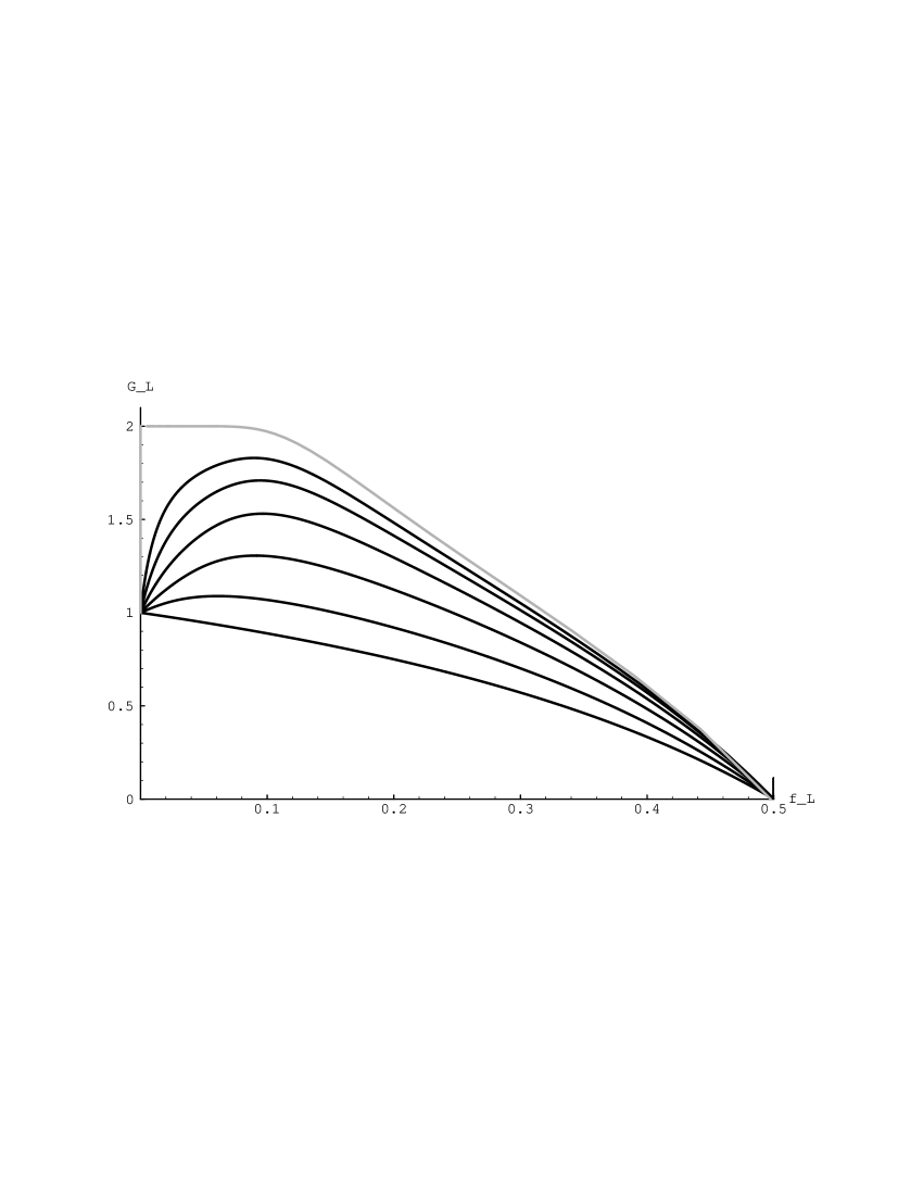
FIG. 3.: $G_{L}$ versus $f$ for several values of $L$. The black curves represent $L$ values from 1 to 6, increasing upward, while the gray curve is the limit as $L\rightarrow\infty$.

Galilean invariance is achieved when $g=1$, or

$\displaystyle G_{L}=\left(1+\frac{2}{D}\right)\left(\frac{n}{n+n_{r}}\right).$

If the quantity $(1+2/D)n/(n+n_{r})$ is greater than the maximum value of $G_{L}$, then galilean invariance is impossible for those values of $D$, $n$, $n_{r}$, and $L$; if it is less than this maximum, then there are two densities at which galilean invariance is achieved. Some of these values are tabulated for the FHP and FCHC lattice gases in Fig. 4.

FHP Lattice Gas ($D=2$, $n=6$)
$n_{r}$	$L$	Low-Density Root	High-Density Root
0	$\infty$	0.0	0.0
1	$6$	0.0396831	0.143848
	$\infty$	0.0	0.168451
2	$4$	0.0704358	0.126560
	$5$	0.0322583	0.177356
	$6$	0.0158730	0.195949
	$\infty$	0.0	0.212636
4	$3$	0.0362392	0.167555
	$4$	0.0166667	0.228582
	$5$	0.0080645	0.253770
	$6$	0.0039683	0.265426
	$\infty$	0.0	0.276535

FCHC Lattice Gas ($D=4$, $n=24$)
$n_{r}$	$L$	Low-Density Root	High-Density Root
0	$4$	0.0704358	0.126560
	$5$	0.0322583	0.177356
	$6$	0.0158730	0.195949
	$\infty$	0.0	0.212636
1	$4$	0.0528917	0.152419
	$5$	0.0253456	0.193030
	$6$	0.0124717	0.209795
	$\infty$	0.0	0.225163
2	$4$	0.0417410	0.171769
	$5$	0.0201613	0.207212
	$6$	0.0099206	0.222576
	$\infty$	0.0	0.236849
4	$3$	0.0654937	0.120009
	$4$	0.0266677	0.203001
	$5$	0.0129032	0.232239
	$6$	0.0063492	0.245488
	$\infty$	0.0	0.257994

FIG. 4.: Values of $f\in(0,1/2)$ such that $g=1$

VIII Viscosity

To compute the viscosity of a ILGA in the Boltzmann molecular chaos approximation [3], we consider its ensemble-averaged collision operator, $\Omega^{i,\ell}$. This quantity is the ensemble average of the increase in bit $\ell$ in direction $i$ due to collisions. It is given by

$\displaystyle\Omega^{i,\ell}=\sum_{s,s^{\prime}}A(s\rightarrow s^{\prime})(s^{\prime i,\ell}-s^{i,\ell}){\cal P}(s),$

where ${\cal P}(s)$ is the probability that the incoming state is $s$, $A(s\rightarrow s^{\prime})$ is the probability that the collision process takes incoming state $s$ to outgoing state $s^{\prime}$, and $s^{i,\ell}$ is the value of bit $\ell$ in direction $i$ in incoming state $s$ (and likewise for outgoing state $s^{\prime}$). In the Boltzmann approximation, the probability of a state $s$ is the product of the corresponding fractional occupation numbers, or their complements,

$\displaystyle{\cal P}(s)=\prod_{k^{\prime}=0}^{n-1}\prod_{\jmath^{\prime}=0}^{L-1}\left(N^{k^{\prime},\jmath^{\prime}}\right)^{s^{k^{\prime},\jmath^{\prime}}}\left(1-N^{k^{\prime},\jmath^{\prime}}\right)^{1-s^{k^{\prime},\jmath^{\prime}}}.$

To get the total increase of particles in direction $i$, we take the sum

$\displaystyle\Omega^{i}\equiv\sum_{\ell=0}^{L-1}2^{\ell}\Omega^{i,\ell}=\sum_{s,s^{\prime}}A(s\rightarrow s^{\prime})(s^{\prime i}-s^{i})\prod_{k^{\prime}=0}^{n-1}\prod_{\jmath^{\prime}=0}^{L-1}\left(N^{k^{\prime},\jmath^{\prime}}\right)^{s^{k^{\prime},\jmath^{\prime}}}\left(1-N^{k^{\prime},\jmath^{\prime}}\right)^{1-s^{k^{\prime},\jmath^{\prime}}},$

where

$\displaystyle s^{i}\equiv\sum_{\ell=0}^{L-1}2^{\ell}s^{i,\ell}$

is the total number of particles in direction $i$ in state $s$ (and likewise for $s^{\prime}$).

To compute the viscosity, we must form the Jacobian matrix of the collision operator. Direct calculation yields

$\displaystyle\frac{\partial\Omega^{i,\ell}}{\partial N^{k,\jmath}}=\sum_{s,s^{\prime}}A(s\rightarrow s^{\prime})(s^{\prime i}-s^{i}){\cal P}(s)\frac{\left(s^{k,\jmath}-N^{k,\jmath}\right)}{N^{k,\jmath}\left(1-N^{k,\jmath}\right)}.$

We would like to evaluate this Jacobian at the equilibrium given by Eq. (V.11),

$\displaystyle N_{0}^{k,\jmath}=\frac{1}{1+(z^{k})^{-2^{\jmath}}}.$

Taking the derivative of this equation with respect to the fugacity,

$\displaystyle\frac{\partial N_{0}^{k,\jmath}}{\partial z^{k}}=\frac{2^{\jmath}(z^{k})^{-2^{\jmath}-1}}{\left[1+(z^{k})^{-2^{\jmath}}\right]^{2}}=\frac{2^{\jmath}N_{0}^{k,\jmath}\left(1-N_{0}^{k,\jmath}\right)}{z^{k}},$

we can use the chain rule to get the integer version of the Jacobian of the collision operator at equilibrium,

$${J}^{i}_{\phantom{{i}}k} \equiv \left.\frac{\partial\Omega^{i}}{\partial N^{k}}\right|_{0}$$ (VIII.20)

$$= \sum_{\ell,\jmath=0}^{L-1}2^{\ell}\;\left.\frac{\partial\Omega^{i,\ell}}{\partial N^{k,\jmath}}\right|_{0}\left.\frac{\partial N^{k,\jmath}/\partial z^{k}}{\partial N^{k}/\partial z^{k}}\right|_{0}$$ (VIII.21)

$$= \sum_{s,s^{\prime}}A(s\rightarrow s^{\prime})(s^{\prime i}-s^{i}){\cal P}_{0}(s)\frac{\left(s^{k}-N^{k}\right)}{z^{k}F_{L}^{\prime}(z^{k})}.$$ (VIII.22)

In fact, we need this result only in the limit of zero Mach number, so we can use the lowest order expression for the fugacity, $z^{k}=z$ (see Sec. VI), which is independent of the index $k$. We find that the zero Mach number limit of the Boltzmann probability of state $s$ is given by

$\displaystyle{\cal P}_{0}(s)=\prod_{k^{\prime}=0}^{n-1}\prod_{\jmath^{\prime}=0}^{L-1}\left(N_{0}^{k^{\prime},\jmath^{\prime}}\right)^{s^{k^{\prime},\jmath^{\prime}}}\left(1-N_{0}^{k^{\prime},\jmath^{\prime}}\right)^{1-s^{k^{\prime},\jmath^{\prime}}}=\prod_{\jmath^{\prime}=0}^{L-1}\left(\frac{1}{1+z^{-2^{\jmath^{\prime}}}}\right)^{p_{\jmath^{\prime}}(s)}\left(\frac{z^{-2^{\jmath^{\prime}}}}{1+z^{-2^{\jmath^{\prime}}}}\right)^{n-p_{\jmath^{\prime}}(s)},$

where

$\displaystyle p_{\jmath}(s)\equiv\sum_{k=0}^{n-1}s^{k,\jmath}$

is the total number of populated bits in the $\jmath$th binary digit. It follows that

$\displaystyle{\cal P}(s)=\left[\prod_{\jmath=0}^{L-1}\left(1+z^{2^{\jmath}}\right)^{-1}\right]^{n}\left(\prod_{\jmath=0}^{L-1}z^{2^{\jmath}p_{\jmath}(s)}\right)=\left(\frac{1-z}{1-z^{2^{L}}}\right)^{n}z^{p(s)},$

where

$\displaystyle p(s)\equiv\sum_{\jmath=0}^{L-1}2^{\jmath}p_{\jmath}(s)$

is the total number of particles present in state $s$.

Inserting this result into the expression, Eq. (VIII.22), for the collision operator, we obtain

$\displaystyle{J}^{i}_{\phantom{{i}}k}=\frac{1}{zF_{L}^{\prime}(z)}\left(\frac{1-z}{1-z^{2^{L}}}\right)^{n}\sum_{s,s^{\prime}}A(s\rightarrow s^{\prime})\left(s^{\prime i}-s^{i}\right)\left[s^{k}-F_{L}(z)\right]z^{p(s)}.$

As a consequence of conservation of probability, Eq. (I.1), and semidetailed balance, Eq. (I.2), it follows that the second term in square brackets vanishes, so we finally get

$\displaystyle{J}^{i}_{\phantom{{i}}k}=\frac{1}{zF_{L}^{\prime}(z)}\left(\frac{1-z}{1-z^{2^{L}}}\right)^{n}\sum_{s,s^{\prime}}A(s\rightarrow s^{\prime})\left(s^{\prime i}-s^{i}\right)s^{k}z^{p(s)}.$

At first order in Knudsen number, the kinetic equation is [4]

$\displaystyle{\bf c}_{i}\cdot\mbox{\boldmath$\nabla$}N_{0}^{i}={J}^{i}_{\phantom{{i}}j}N_{1}^{j},$

where there is an understood summation over $j$. The only part of the left-hand side that contributes to the viscosity comes from the second term on the right-hand side of Eq. (VI.16), whence

$\displaystyle{J}^{i}_{\phantom{{i}}j}N_{1}^{j}=\frac{1}{A_{2}}{\bf c}_{i}{\bf c}_{i}:\mbox{\boldmath$\nabla$}{\bf u}.$

Now, $J$ is a singular matrix; it has a null eigenvector corresponding to each hydrodynamic mode of the system. These null eigenvectors span what we shall call the hydrodynamic subspace of the system. The complement of this subspace is called the kinetic subspace, and is spanned by the kinetic modes with nonzero (negative) eigenvalue. If we restrict our attention to the kinetic subspace, then we can form the pseudoinverse of $J$, denoted by $J^{-1}$, in terms of which we may write

$\displaystyle N_{1}^{i}=\frac{1}{A_{2}}{\left(J^{-1}\right)}^{i}_{\phantom{{i}}j}{\bf c}_{j}{\bf c}_{j}:\mbox{\boldmath$\nabla$}{\bf u}.$

The conservation law for momentum then contains the term

$$\sum_{i}\left({\bf c}_{i}{\bf c}_{i}\cdot\mbox{\boldmath$\nabla$}N_{1}^{i}+\mbox{$\frac{1}{2}$}{\bf c}_{i}{\bf c}_{i}{\bf c}_{i}:\mbox{\boldmath$\nabla$}\mbox{\boldmath$\nabla$}N_{0}^{i}+\cdots\right)$$

$$= \mbox{\boldmath$\nabla$}\cdot\left\{\frac{1}{A_{2}}\left[\sum_{i,j}{\bf c}_{i}{\bf c}_{i}{\left(J^{-1}\right)}^{i}_{\phantom{{i}}j}{\bf c}_{j}{\bf c}_{j}+\mbox{$\frac{1}{2}$}\sum_{i}{\bf c}_{i}{\bf c}_{i}{\bf c}_{i}{\bf c}_{i}\right]:\left(\mbox{\boldmath$\nabla$}{\bf u}\right)\right\}+\cdots.$$

We note that $J^{-1}$ is diagonalized and degenerate in the subspace spanned by the $n$ outer products of the lattice vectors with themselves; that is

$$\sum_{j}{\left(J^{-1}\right)}^{i}_{\phantom{{i}}j}{\bf c}_{j}{\bf c}_{j}=-\lambda{\bf c}_{i}{\bf c}_{i},$$ (VIII.23)

where $\lambda$ is a scalar, whence the above term in the momentum conservation equation becomes

$\displaystyle\mbox{\boldmath$\nabla$}\cdot\left[\frac{A_{4}}{A_{2}}\left(-\lambda+\mbox{$\frac{1}{2}$}\right){\bf 1}_{4}:\left(\mbox{\boldmath$\nabla$}{\bf u}\right)\right]+\cdots=\mbox{\boldmath$\nabla$}\cdot\left[\frac{A_{4}}{A_{2}}\left(-\lambda+\mbox{$\frac{1}{2}$}\right)\mbox{\boldmath$\nabla$}{\bf u}\right],$

from which we identify the kinematic viscosity,

$\displaystyle\nu=\frac{A_{4}}{A_{2}}\left(\lambda-\mbox{$\frac{1}{2}$}\right).$

The quantity $\lambda$ is then determined by taking the double spatial dot product of ${\bf c}_{i}{\bf c}_{i}$ on both sides of Eq. (VIII.23), and summing over $i$ to get

$\displaystyle n=-\lambda\sum_{i,j}{J}^{i}_{\phantom{{i}}j}\left({\bf c}_{i}\cdot{\bf c}_{j}\right)^{2},$

whence

$\displaystyle\frac{1}{\lambda}=\frac{-1}{nzF_{L}^{\prime}(z)}\left(\frac{1-z}{1-z^{2^{L}}}\right)^{n}\sum_{i,j}\sum_{s,s^{\prime}}A(s\rightarrow s^{\prime})\left(s^{\prime i}-s^{i}\right)z^{p(s)}s^{j}\left({\bf c}_{i}\cdot{\bf c}_{j}\right)^{2},$

where $f=f_{L}(z)$ determines the parameter $z$ in terms of the fractional occupation number. This result is easily seen to reduce to that of Hénon [12] when $L=1$.

We computed the viscosity of an $L=2$ lattice gas in two dimensions ($D=2$) by measuring the decay of a shear wave in periodic geometry. We used a lattice of size $512\times 512$ on a CAM-8 Cellular-Automata Machine [13]. The probabilistic collision procedure used obeyed semi-detailed balance, with each outgoing state allowed by the conservation laws sampled with equal probability. Fig. 5 shows the decay of the shear wave amplitude to be exponential in nature, as is appropriate for Navier-Stokes evolution. The time constant of the exponential then determines the viscosity, which is plotted as a function of density in Fig. 6, along with the curve predicted by the theory given above.

FIG. 5.: Time decay of shear-wave amplitude

FIG. 6.: Viscosity versus $f$ for $L=2$.

While the agreement with theory is good at intermediate values of the fractional occupation number near half filling, we note that it is seriously in error at low (and high) fractional occupation numbers. At present, we attribute this discrepency to deviations from the Boltzmann molecular chaos approximation, and we plan to investigate them using kinetic ring theory [4] in a forthcoming publication.

IX Statistical Noise

Finally, we consider the statistical noise of the ILGA model. With the maximum number of particles per direction increasing as $2^{L}$, one might naively expect the noise level to decrease with $L$ as $1/\sqrt{2^{L}}\sim 2^{-L/2}$. Unfortunately, as we shall show, this expectation is not realized, due to the extremely narrow dynamic range of the fugacity for large $L$. This is best seen in Fig. 1, in which the effective width of the function $f_{L}(z)$ near $z=\mbox{$\frac{1}{2}$}$ decreases like $2^{-L}$, making for a subtle limiting process that is discussed in Appendix B.

Let $n^{i,\ell}({\bf x},t)$ be the precise value of bit $\ell$ in direction $i$ at lattice site ${\bf x}$ at time $t$. The ensemble-average of this quantity is $N^{i,\ell}$, as used in the text of the paper. The mean number of particles in a (space-time) block of $N$ sites is then

$\displaystyle{\cal F}_{1}=\sum_{({\bf x},t)}^{N}\sum_{i}^{n}\sum_{\ell=0}^{L-1}2^{\ell}\left\langle n^{i,\ell}({\bf x},t)\right\rangle=nNF_{L}(z),$

where the angle brackets denote the ensemble average.

The mean square of the number of particles in this block of sites is then

$\displaystyle{\cal F}_{2}=\sum_{({\bf x},t)}^{N}\sum_{({\bf x}^{\prime},t^{\prime})}^{N}\sum_{i}^{n}\sum_{i^{\prime}}^{n}\sum_{\ell=0}^{L-1}\sum_{\ell^{\prime}=0}^{L-1}2^{\ell+\ell^{\prime}}\left\langle n^{i,\ell}({\bf x},t)n^{i^{\prime},\ell^{\prime}}({\bf x}^{\prime},t^{\prime})\right\rangle.$

The bits are either zero or one, and in the Boltzmann molecular chaos approximation different bits are uncorrelated. It follows that

$\displaystyle\left\langle n^{i,\ell}({\bf x},t)n^{i^{\prime},\ell^{\prime}}({\bf x}^{\prime},t^{\prime})\right\rangle=\left\langle n^{i,\ell}({\bf x},t)\right\rangle\left\langle n^{i^{\prime},\ell^{\prime}}({\bf x}^{\prime},t^{\prime})\right\rangle+\delta_{{\bf x},{\bf x}^{\prime}}\delta_{t,t^{\prime}}\delta_{i,i^{\prime}}\delta_{\ell,\ell^{\prime}}\left\langle n^{i,\ell}({\bf x},t)\right\rangle\left(1-\left\langle n^{i,\ell}({\bf x},t)\right\rangle\right),$

whence

$\displaystyle{\cal F}_{2}={\cal F}_{1}^{2}+nN\sum_{\ell}^{L-1}\frac{2^{2\ell}z^{2^{\ell}}}{\left(1+z^{2^{\ell}}\right)^{2}}={\cal F}_{1}^{2}+nNzF_{L}^{\prime}(z).$

It follows that the standard deviation of the number of particles in the block is $\sqrt{{\cal F}_{2}-{\cal F}_{1}^{2}}$. To define a fractional noise, we could divide this by the mean number of particles, ${\cal F}_{1}$, but it preserves particle-hole symmetry if we instead divide it by the square root of the product of the mean number of particles and the mean number of holes, thus

$$\Delta{\cal F}\equiv\sqrt{\frac{{\cal F}_{2}-{\cal F}_{1}^{2}}{{\cal F}_{1}\left[nN\left(2^{L}-1\right)-{\cal F}_{1}\right]}}=\frac{1}{\sqrt{nN\left(2^{L}-1\right)}}\sqrt{\frac{zf_{L}^{\prime}(z)}{f_{L}(z)\left[1-f_{L}(z)\right]}}.$$ (IX.24)

This appears to decrease exponentially with $L$, but it must be noted that the logarithmic derivative of $f_{L}(z)$ goes as $2^{L}$ at $z=\mbox{$\frac{1}{2}$}$. Since, for fixed fractional occupation number $f_{L}$, $z$ tends to $\frac{1}{2}$ as $L$ tends to infinity, we see that $\Delta{\cal F}$ is order unity in $L$. Thus, the fractional noise does decrease with $L$, but not as rapidly as one might hope. It is plotted for several different values of $L$ in Fig. 7.

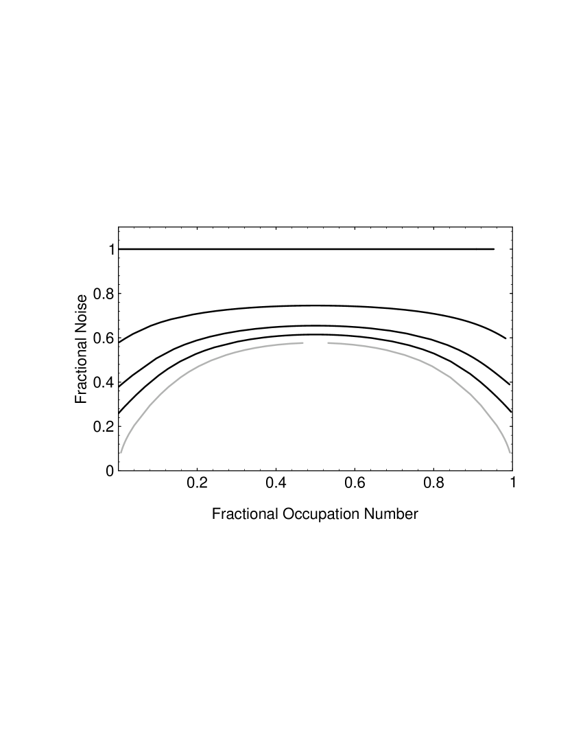
FIG. 7.: $\Delta{\cal F}_{L}$ versus $f$ for several values of $L$. The black curves represent $L$ values from 1 to 6, increasing downward, while the gray curve is the limit as $L\rightarrow\infty$.

X Sampling Procedure

Finally, we consider some practical considerations concerning the computer implementation of the ILGA model. Since each site has $nL$ bits, and therefore $2^{nL}$ possible states, and since the most popular lattices with the requisite isotropy properties have $n=6$ and $n=24$, it is clear that the brute-force approach in which a lookup table is used to store the collision outcome states will not be feasible for $L$ much greater than unity.

For this reason, we propose another sampling scheme for the outgoing states. Though the method we propose is completely general, we illustrate it for the two dimensional integer lattice gas on a triangular grid ($n=6$). Let ${\bf n}$ be an integer-valued column $n$-vector whose components are the particle occupation numbers in each of the six directions.

Let us suppose that the mass and the two components of momentum are the only conserved quantities. Since these conserved quantitites are linear in the particle occupation numbers, each of them correspond to a row vector, whose inner product with ${\bf n}$ yields the conserved quantity in question. Thus, corresponding to the mass we have the row vector

$\displaystyle{\bf q}_{1}=\left(\begin{array}[]{rrrrrr}1&1&1&1&1&1\end{array}\right),$

corresponding to the $x$-momentum (multiplied by a factor of $2$), we have

$\displaystyle{\bf q}_{2}=\left(\begin{array}[]{rrrrrr}2&1&-1&-2&-1&1\end{array}\right),$

and corresponding to the $y$-momentum (multiplied by a factor of $2/\sqrt{3}$), we have

$\displaystyle{\bf q}_{3}=\left(\begin{array}[]{rrrrrr}0&1&1&0&-1&-1\end{array}\right).$

In fact, these row vectors are precisely the hydrodynamic eigenvectors, mentioned in our derivation of the viscosity; that is,

$\displaystyle{J}^{i}_{\phantom{{i}}k}({\bf q}_{1})^{k}={J}^{i}_{\phantom{{i}}k}({\bf q}_{2})^{k}={J}^{i}_{\phantom{{i}}k}({\bf q}_{3})^{k}=0.$

It is clear that these can always be chosen to be mutually orthogonal, without loss of generality. Using the Gram-Schmidt procedure, it is then possible to find three vectors spanning the kinetic subspace, orthogonal to the above; e.g.,

$\displaystyle{\bf q}_{4}=\left(\begin{array}[]{rrrrrr}2&-1&-1&2&-1&-1\end{array}\right),$

$\displaystyle{\bf q}_{5}=\left(\begin{array}[]{rrrrrr}1&-1&1&-1&1&-1\end{array}\right),$

and

$\displaystyle{\bf q}_{6}=\left(\begin{array}[]{rrrrrr}0&1&-1&0&1&-1\end{array}\right).$

Now the collision process takes state ${\bf n}$ to state ${\bf n}^{\prime}$. Since it cannot change the values of the conserved quantities, it follows that the difference between ${\bf n}^{\prime}$ and ${\bf n}$ must be a linear combination of kinetic eigenvectors. That is,

$\displaystyle{\bf n}^{\prime}={\bf n}+\alpha_{4}{\bf q}_{4}^{T}+\alpha_{5}{\bf q}_{5}^{T}+\alpha_{6}{\bf q}_{6}^{T},$

where the $\alpha$’s are integer constants, and where the superscript $T$ denotes “transpose.” Thus, writing out components, we have

$\displaystyle{\bf n}^{\prime}=\left(\begin{array}[]{l}n_{1}+2\alpha_{4}+\alpha_{5}\\ n_{2}-\alpha_{4}-\alpha_{5}+\alpha_{6}\\ n_{3}-\alpha_{4}+\alpha_{5}-\alpha_{6}\\ n_{4}+2\alpha_{4}-\alpha_{5}\\ n_{5}-\alpha_{4}+\alpha_{5}+\alpha_{6}\\ n_{6}-\alpha_{4}-\alpha_{5}-\alpha_{6}\end{array}\right).$

Since the components of ${\bf n}^{\prime}$ must all be between $0$ and $2^{L}-1$, inclusive, we derive the following six inequality constraints:

$$0 \leq n_{1}+2\alpha_{4}+\alpha_{5}\leq 2^{L}-1$$

$$0 \leq n_{2}-\alpha_{4}-\alpha_{5}+\alpha_{6}\leq 2^{L}-1$$

$$0 \leq n_{3}-\alpha_{4}+\alpha_{5}-\alpha_{6}\leq 2^{L}-1$$

$$0 \leq n_{4}+2\alpha_{4}-\alpha_{5}\leq 2^{L}-1$$

$$0 \leq n_{5}-\alpha_{4}+\alpha_{5}+\alpha_{6}\leq 2^{L}-1$$

$$0 \leq n_{6}-\alpha_{4}-\alpha_{5}-\alpha_{6}\leq 2^{L}-1.$$

These inequality constraints define a polytope in the three dimensional space of allowed values of $\alpha_{4}$, $\alpha_{5}$ and $\alpha_{6}$. We know that this polytope must exist and contain the origin in that space, since $\alpha_{4}=\alpha_{5}=\alpha_{6}=0$, corresponding to the “trivial collision” in which the occupation numbers do not change their values, will always satisfy the constraints.

The collision process is then specified by a strategy for sampling points from this polytope. One viable strategy which certainly satisfies semidetailed balance is to sample the points within this polytope uniformly. It is possible, though tedious, to derive a closed-form algorithm to do this, based on the above constraints. Alternatively, with some loss of efficiency, one can simply bound the polytope and use a rejection sampling scheme. Details of this procedure will be provided in a forthcoming publication [14].

XI Conclusions

We have generalized the hydrodynamic lattice gas model to include integer numbers of particles moving in each direction at each site. We have presented the thermodynamics and kinetic theory of this generalized Integer Lattice Gas (ILGA) model, including closed-form (or parametric algebraic) equations for the equilibrium distribution function, the entropy, the equation of state, the non-galilean factor in the inertial term of the fluid equations, and the statistical noise. We have thereby shown that the ILGA model allows for the attainment of galilean invariance, and a reduction in the kinematic viscosity and the statistical noise. In future publications, we shall show that this generalization also allows for more straightforward inclusion of interparticle interactions than the usual binary model.

A Closed-Form Expression for $F_{L}(z)$

In this Appendix, we prove Eq. (V.13), where $F_{L}(z)$ is defined by Eq. (V.12). Using mathematical induction, we first note that the statement of the theorem is true for $L=1$:

$$F_{1}(z) \equiv \sum_{\ell=0}^{0}\frac{2^{\ell}}{1+z^{-2^{\ell}}}=\frac{1}{1+z^{-1}}=\frac{z}{1+z}=\frac{z(1-z)}{1-z^{2}}$$

$$= \frac{z(1+z)}{1-z^{2}}-\frac{2z^{2}}{1-z^{2}}=\frac{z}{1-z}-\frac{2z^{2}}{1-z^{2}}.$$

Next, we assume the truth of the statement for $L=K$:

$\displaystyle F_{K}(z)\equiv\sum_{\ell=0}^{K-1}\frac{2^{\ell}}{1+z^{-2^{\ell}}}=\frac{z}{1-z}-\frac{2^{K}z^{2^{K}}}{1-z^{2^{K}}}.$

It follows that

$$F_{K+1}(z) \equiv \sum_{\ell=0}^{K}\frac{2^{\ell}}{1+z^{-2^{\ell}}}=F_{K}(z)+\frac{2^{K}}{1+z^{-2^{K}}}$$

$$= \frac{z}{1-z}-\frac{2^{K}z^{2^{K}}}{1-z^{2^{K}}}+\frac{2^{K}}{1+z^{-2^{K}}}=\frac{z}{1-z}+2^{K}\left(\frac{1}{1-z^{-2^{K}}}+\frac{1}{1+z^{-2^{K}}}\right)$$

$$= \frac{z}{1-z}+2^{K}\frac{2}{1-\left(z^{-2^{K}}\right)^{2}}=\frac{z}{1-z}+\frac{2^{K+1}}{1-z^{-2^{K+1}}}$$

$$= \frac{z}{1-z}-\frac{2^{K+1}z^{2^{K+1}}}{1-z^{2^{K+1}}},$$

and we have thereby proven the theorem for all $K$.

Alternatively, we may simply note that the summation can be written in the telescoping form

$\displaystyle F_{L}(z)\equiv\sum_{\ell=0}^{L-1}\frac{2^{\ell}}{1+z^{-2^{\ell}}}=\sum_{\ell=0}^{L-1}\left(\frac{2^{\ell}z^{2^{\ell}}}{1-z^{2^{\ell}}}-\frac{2^{\ell+1}z^{2^{\ell+1}}}{1-z^{2^{\ell+1}}}\right),$

from which the result follows immediately.

B The Infinite Integer Limit

To consider the limit of infinite integers, $L\rightarrow\infty$, we first note that the fractional occupation number,

$$f_{L}(z)=\frac{F_{L}(z)}{2^{L}-1}=\frac{1}{2^{L}-1}\left(\frac{z}{1-z}-\frac{2^{L}z^{2^{L}}}{1-z^{2^{L}}}\right),$$ (B.1)

has the limiting behavior

$\displaystyle\lim_{z\rightarrow 0}f_{L}(z)=0$

$\displaystyle\lim_{z\rightarrow 1}f_{L}(z)=\mbox{{$\frac{1}{2}$}}$

$\displaystyle\lim_{z\rightarrow\infty}f_{L}(z)=1$

for all $L$; here we have used L’Hôpital’s rule to establish the result for $z\rightarrow 1$. Referring to Figure 1, we note that the function $f_{L}(z)$ becomes increasingly like a step at $z=1$ as $L\rightarrow\infty$. To verify this, we note that the width of the gradient there can be estimated by

$\displaystyle\lim_{z\rightarrow 1}\frac{f_{L}(z)}{f_{L}^{\prime}(z)}=\frac{6}{2^{L}+1},$

which clearly goes to zero as $L\rightarrow\infty$; once again we have used L’Hôpital’s rule to establish this result.

The approach to a step function means that the entire range of fractional occupation numbers is parametrized by values of $z$ within order $2^{-L}$ from $1$, as $L\rightarrow\infty$. That being the case, we write

$$z=1+\frac{y}{2^{L}},$$ (B.2)

where $y$ is a new parameter of order unity. Note that the fractional occupation number is exactly $1/2$ when $y=0$. Inserting Eq. (B.2) into Eq. (B.1), we can now take the limit as $L\rightarrow\infty$ to get

$$\lim_{L\rightarrow\infty}f_{L}\left(1+\frac{y}{2^{L}}\right)=\frac{1}{1-e^{-y}}-\frac{1}{y}.$$ (B.3)

Next, inserting Eq. (B.2) into Eqs. (IV.9) and (IV.10), and taking the limit as $L\rightarrow\infty$, we find the entropy excess,

$$\lim_{L\rightarrow\infty}\Delta S_{L}\left(1+\frac{y}{2^{L}}\right)=\ln\left(1-e^{-y}\right)-\frac{ye^{-y}}{1-e^{-y}}-\ln y+1.$$ (B.4)

Eqs. (B.3) and (B.4) constitute parametric algebraic equations, with parameter $y$, yielding $\Delta S_{L}$ as a function of the fractional occupation number $f_{L}$ as $L\rightarrow\infty$. These equations were used to produce the shaded curve in Fig. 2.

Likewise, inserting Eq. (B.2) into Eqs. (IX.24), and taking the limit as $L\rightarrow\infty$, we find the fractional noise,

$$\lim_{L\rightarrow\infty}\Delta{\cal F}_{L}\left(1+\frac{y}{2^{L}}\right)=\sqrt{\frac{y^{2}-2\cosh y+2}{y^{2}-2y\sinh y+2\cosh y-2}}$$ (B.5)

Eqs. (B.3) and (B.5) constitute parametric algebraic equations, with parameter $y$, yielding $\Delta{\cal F}_{L}$ as a function of the fractional occupation number $f_{L}$ as $L\rightarrow\infty$. These equations were used to produce the shaded curve in Fig. 7.

Finally, inserting Eq. (B.2) into Eqs. (VII.19), and taking the limit as $L\rightarrow\infty$, we find the $G_{L}$ factor for a Bravais lattice,

$$\lim_{L\rightarrow\infty}G_{L}\left(1+\frac{y}{2^{L}}\right)=\frac{2+\left(y^{3}+2y-8\right)e^{y}+\left(y^{4}-6y+12\right)e^{2y}+\left(y^{4}-y^{3}+6y-8\right)e^{3y}-2\left(y-1\right)e^{4y}}{\left[1-(y^{2}+2)e^{y}+e^{2y}\right]^{2}}.$$ (B.6)

Eqs. (B.3) and (B.6) constitute parametric algebraic equations, with parameter $y$, yielding $G_{L}$ as a function of the fractional occupation number $f_{L}$ as $L\rightarrow\infty$. These equations were used to produce the shaded curve in Fig. 3.

REFERENCES

• [1] Frisch, U., Hasslacher, B., Pomeau, Y., Phys. Rev. Lett. 56 (1986).
• [2] Wolfram, S., J. Stat. Phys., 45 (1986) 471.
• [3] Frisch, U., dโ€™Humiรจres, D., Hasslacher, B., Lallemand, P., Pomeau, Y., Rivet, J.-P., Complex Systems 1 (1987) 75-136.
• [4] Boghosian, B.M., Taylor, W., Phys. Rev. E 52 (1995) 510-554.
• [5] Cercignani, C., โ€œThe Boltzmann Equation and its Applications,โ€ Springer-Verlag (1988). See pp. 232-261.
• [6] Landau, L.D., Lifshitz, E.M., โ€œFluid Mechanics,โ€ Pergamon Press (1982 edition). See page 24.
• [7] dโ€™Humiรจres, D., Lallemand, P., Complex Systems 1 (1987) 633-647.
• [8] Gunstensen, A.K., Rothman, D.H., Zaleski, S., Zanetti, G., Phys. Rev. A 43 (1991) 4320-4327.
• [9] Benzi, R., Succi, S., Vergassola, M., Physics Reports 222 (1992) 145-197.
• [10] Ladd, A.J.C., Phys. Rev. Lett. 70 (1993) 1339; Ladd, A.J.C., J. Fluid Mech. 271 (1994) 285; Ladd, A.J.C., J. Fluid Mech. 271 (1994) 311.
• [11] Chen, H-D., Chen, S-Y., Matthaeus, W.H., Phys. Rev. A 45 (1992) R5339-R5342; Qian, Y-H., Dโ€™Humiรจres, D., Lallemand, P., Europhys. Lett. 17 (1992) 479-484.
• [12] Hรฉnon, M., Complex Systems 1 (1987) 763.
• [13] Rothman, D.H., Margolus, N.H., Adler, C., Boghosian, B.M., Flekkoy, E., J. Stat. Phys. 81 (October, 1995).
• [14] Boghosian, B.M., Yepez, J., Alexander, F.J., in preparation.