A Dynamical Theory of Electron Transfer: Crossover from Weak to Strong Electronic Coupling

Abstract

We present a real-time path integral theory for the rate of electron transfer reactions. Using graph theoretic techniques, the dynamics is expressed in a formally exact way as a set of integral equations. With a simple approximation for the self-energy, the rate can then be computed analytically to all orders in the electronic coupling matrix element. We present results for the crossover region between weak (nonadiabatic) and strong (adiabatic) electronic coupling and show that this theory provides a rigorous justification for the salient features of the rate expected within conventional electron transfer theory. Nonetheless, we find distinct characteristics of quantum behavior even in the strongly adiabatic limit where classical rate theory is conventionally thought to be applicable. To our knowledge, this theory is the first systematic dynamical treatment of the full crossover region.

I Introduction

Since the landmark papers of Marcus [1, 2] on the theory of electron transfer (ET) reactions, the central role of the solvent in determining the ET rate has been well recognized. The ordinary ET reaction is an activated process [2], in which there is a free energy barrier separating reactants and products. This barrier is the result of the often strongly solvated donor and acceptor states, and the transfer of an electron then requires a specific large-scale reorganization of the environment, usually achieved through equilibrium fluctuations.

ET reactions are commonly thought to be well understood in two distinct limits (see Fig. 1). First, for a very weak electronic coupling or the so-called nonadiabatic limit, the ET can be treated with a perturbation theory [2], which to lowest order in the electronic coupling leads to the Golden Rule expression for the rate. For the opposite adiabatic limit in which the electronic coupling is large, the rate is thought to be controlled by the motion of the solvent on the lower electronic state and well described by classical activated rate theory [2]. In both nonadiabatic and adiabatic theories, there is an assumed separation of timescales between the motions of the electron and the solvent. In the nonadiabatic limit, the solvent fluctuations are assumed fast and the ET is controlled by thermal excitations of the solvent to near the crossing region followed by a fast transversal of the crossing region by the solvent. The ET rate is therefore controlled by the probability of an electronic transition proportional to the square of the electronic coupling. The adiabatic limit on the other hand is characterized by slow solvent fluctuations such that the Born-Oppenheimer approximation for the electron can be invoked. Therefore according to conventional theories in these two limits, the ET rate is expected to depend on the electronic coupling $\hbar\Delta/2$ like

$$k_{\rm ET}\sim\left\{\begin{array}[]{ll}\Delta^{2}\exp(-E_{0}/kT),&\mbox{nonadiabatic}\\ \exp(-[E_{0}-\hbar\Delta/2]/kT),&\mbox{adiabatic}\end{array}\right.$$ (1)

where $T$ is the temperature and $k$ is the Boltzmann constant.

Regarding the assumed separation of timescales, there are at least two aspects of ET reactions which remain largely unclear and demand more complete theoretical treatments. First, there is the question of the “crossover region”. By this we mean the region between the nonadiabatic and the adiabatic limits in which the electronic matrix element changes from the weak coupling to the strong coupling limit. In this region, the assumed separation of timescales is necessarily violated. In fact, a successful dynamical crossover theory that can unify the two limits requires inclusion of high order electronic coupling terms [3, 4, 5], and such a theory has yet to be found. Second, as is true in almost all condensed phase ET reactions, the frequency spectrum of solvent motions is charac- FIG. 1.: Potential surfaces for nonadiabatic (a) and adiabatic (b) electron transfer. In the nonadiabatic case, the Landau-Zener mechanism facilitates transfer at the crossing point of two diabatic surfaces. The adiabatic transfer is often described as a barrier crossing on the lower adiabatic energy surface. terized by a broad distribution of timescales. Hence, the assumption of timescale separation, while perhaps true for parts of the spectrum, may not be so for others. While it is commonly believed that fast solvent polarization has little effect on the ET rate [2, 6], unconventional behaviors have been suggested for solvents with high-frequency modes [7]. Indeed, Stuchebrukhov and Song [8] have recently reported that high-frequency components in the solvent spectrum can substantially renormalize the intrinsic electronic coupling to slow down the otherwise adiabatic rate. The same adiabatic renormalization effects have also been recognized by others in a somewhat different context [9, 10]. The questions surrounding the influence of high-frequency modes in adiabatic reactions seem far from settled.

The search for a unified treatment that can connect the conventional nonadiabatic and adiabatic theories presents a considerable challenge. Early attempts were made by Levich [11] and Zusman [12] to use the Landau-Zener formula to incorporate higher-order effects in the electronic coupling into the ET rate. Along a similar line of thinking, Garg, Onuchic and Ambegaokar [3] used an approximate real-time path integral treatment in an attempt to account for adiabaticity effects.

More recent approaches [13, 14, 8, 15] have been largely based on an imaginary-time formulation of the problem. Most noticeable of these is the centroid free energy method [16] employed by Gehlen et al. [13, 14]. Extensions of this to complex-valued centroid coordinates by Stuchebrukhov and Song [8] have also been useful for obtaining results for the inverted region where nuclear tunneling is crucial. Another imaginary-time theory which does not explicitly employ the centroid formulation has been given by Cao et al. [15] who focus on the computational aspects of instanton methods. All these theories rely on an assumed relationship between the ET rate and an analytic continuation of the partition function for the tunneling system [23]. This relationship, however has not been derived from first principles for the ET problem.

In this paper, we take a rather different approach to the problem. With a spin-boson model for the ET reaction, our method sets out from an exact path integral formulation [10, 17] for the real-time dynamics of the electron. From the path integrals, it is then easy to see that the ET rate is related to clusters of kink/anti-kink pairs (called “blips”) [10] which interact with each other through a nonlocal influence functional. When the fluctuations of the bath polarization are sufficiently fast compared to the motions of the electron, these interblip interactions vanish. In this case, the rate reduces to nonadiabatic theory and becomes completely equivalent to a low-order perturbation theory in the electronic coupling. On the other hand, when the bath motions are sufficiently slow compared to the electron, interblip interactions force blips to bunch up into clusters. In each cluster, multiple electronic transitions are possible, and the rate is now given by a series containing high-order terms in the electronic coupling. Using standard graph theoretic techniques and a simple approximation for the self-energy (i.e., the sum over all irreducible diagrams), we are able to sum up an infinite number of terms in this series and obtain an expression for the ET rate not only in the nonadiabatic and adiabatic limits, but for the entire crossover region. To our knowledge, this is the first successful real-time formulation that can span the whole crossover region.

Section II gives a brief overview of the path-integral formulation of the dynamics of the spin-boson system. With minor modification, this material follow closely reviews by Leggett [10] and Weiss [17]. In Section III, the formal expression for the time-dependent dynamics is transformed diagrammatically to yield a rigorous result for the ET rate. Sections III A and III B give a pictorial interpretation of the results, and Section III C discusses general ET behaviors in the two limits in terms of topological features of the graphs. Section III D presents a simple approximation which allows us to resum the entire perturbation series for the entire crossover region. Some numerical results for the crossover behavior are also discussed. Finally, section IV concludes this paper with a brief summary of the most important features of the present theory and our results.

II Dynamics of Electron Transfer in the Spin-Boson Model

For the discussion of ET dynamics in a donor-acceptor system in the condensed phase, we take the simple spin-boson model which has been used in many previous studies. The Hamiltonian is

$$H=H_{\rm S}+H_{\rm I}+H_{\rm B}\;,$$ (2)

where

$$H_{\rm S} = -{\hbar\over 2}\left(\Delta\sigma_{x}+\epsilon\sigma_{z}\right)\;,$$ (3)

$$H_{\rm I} = -{a\over 2}\sigma_{z}\sum_{\alpha}c_{\alpha}x_{\alpha}\;,$$ (4)

$$H_{\rm B} = {1\over 2}\sum_{\alpha}{p_{\alpha}^{2}\over m_{\alpha}}+m_{\alpha}\omega_{\alpha}^{2}x_{\alpha}^{2}\;,$$ (5)

defining two localized electronic states (with a possible asymmetry $\epsilon$) and their overlap in the tight-binding approximation with a bilinear coupling to a number of solvent modes, which are assumed harmonic.

Only two quantities of the oscillator bath are relevant to the dynamics of the electron. They are the temperature associated with the initial thermal density matrix of the bath, and its spectral density

$$J(\omega)={\pi\over 2}\sum_{\alpha}{c_{\alpha}^{2}\over m_{\alpha}\omega_{\alpha}}\delta(\omega-\omega_{\alpha})\;.$$ (6)

A commonly used form of $J(\omega)$, which in the classical limit describes a frequency-independent friction, is the ohmic spectral density

$${a^{2}\over 2\pi\hbar}\,J(\omega)=\alpha\omega e^{-{\omega/\omega_{c}}}\;,$$ (7)

where $\alpha$ is a dimensionless parameter which characterizes the strength of the dissipation. We shall use this spectral density throughout this paper. Classically, the ohmic bath is characterized by a single parameter – the reorganization energy $\hbar\Lambda=2\alpha\hbar\omega_{c}$.

Using standard path-integral techniques [18, 10, 17, 3], a partial trace can be performed over the oscillator coordinates to eliminate them from the problem. One is left with an effective double path integral expression for the dynamics of the reduced density matrix for the electron.

The forward- and reverse-time paths for the electron $\sigma(t)$ and $\sigma^{\prime}(t)$ are piecewise constant functions of time, alternating between the two allowed values $\pm 1$. This particular class of functions can obviously be parametrized by the number of transitions between the two allowed values, the times at which these transitions occur, and the constant values the function assumes in the intervening intervals.

Applying this parametrization, and replacing $\sigma(t)$ and $\sigma^{\prime}(t)$ with symmetrized and antisymmetrized coordinates $\xi(t)=(\sigma(t)-\sigma^{\prime}(t))/2$ and $\eta(t)=(\sigma(t)+\sigma^{\prime}(t))/2$, an exact path-integral expression for the transition probability from position $\sigma_{i}$ to $\sigma_{f}$ can be written as [10, 17]

$$P_{\sigma_{i}\sigma_{f}}(t) = \delta_{\sigma_{i},\sigma_{f}}+\sigma_{i}\sigma_{f}\sum_{n=1}^{\infty}\left(-\frac{\Delta^{2}}{4}\right)^{n}$$ (9)

$$\times\int\limits_{0}^{t}{\cal D}_{n}\{t_{j}\}\sum_{\{\xi_{j},\eta_{j}=\pm 1\}}\prod_{l=1}^{n}B_{l}\prod_{k=1}^{l-1}F_{lk}\;,$$

where we have used the shorthand notation

$$\int\limits_{0}^{t}{\cal D}_{n}\{t_{j}\}\equiv\int\limits_{0}^{t}dt_{2n}\int\limits_{0}^{t_{2n}}dt_{2n-1}\ldots\int\limits_{0}^{t_{2}}dt_{1}$$ (10)

for the time-ordered integrals. The $\{t_{j}\}$ here are the times at which transitions are made on the $\xi(t)$ and $\eta(t)$ paths and denoting the directions of these transitions by $\xi_{j}$ and $\eta_{j}$ (called “charges”), the interaction terms $B_{l}$ and $F_{lk}$ are related to the real and imaginary part of the twice-integrated bath correlation function in the following way

$$S(t)+iR(t) = \frac{a^{2}}{\pi\hbar}\int\limits_{0}^{\infty}d\omega\frac{J(\omega)}{\omega^{2}}\Bigg{[}(1-\cos\omega t)\coth\left(\frac{\hbar\beta\omega}{2}\right)$$ (12)

$$\hskip 100.00015pt+\,i\sin\omega t\Bigg{]}$$

through

$$B_{l} = \exp(-\xi_{2l-1}\xi_{2l}S_{2l,2l-1}+i\xi_{2l-1}\epsilon(t_{2l}-t_{2l-1})$$ (14)

$$+i\xi_{2l}\eta_{2l-1}R_{2l,2l-1})\;,$$

and

$$F_{lk} = \exp\left(-\xi_{2l}\xi_{2k-1}S_{2l,2k-1}\right.-\xi_{2l-1}\xi_{2k}S_{2l-1,2k}$$ (18)

$$-\xi_{2l}\xi_{2k}S_{2l,2k}\left.-\xi_{2l-1}\xi_{2k-1}S_{2l-1,2k-1}\right)$$

$$\exp\left(i\xi_{2l}\eta_{2k-1}R_{2l,2k-1}\right.+i\xi_{2l-1}\eta_{2k-1}R_{2l-1,2k-1})$$

$$+i\xi_{2l}\eta_{2k}R_{2l,2k}\left.+i\xi_{2l-1}\eta_{2k}R_{2l-1,2k}\right)\;,$$

where $S_{mn}\equiv S(t_{m}-t_{n})$ and $R_{mn}\equiv R(t_{m}-t_{n})$. Because of the two-state nature of the electron coordinate, the charges are constrained such that $\xi_{2l-1}=-\xi_{2l}$ and $\eta_{2l}=-\eta_{2l+1}$. These constraints imply that there are two kinds of time intervals on the double path – those intervals with $\sigma=\sigma^{\prime}$ (dubbed ‘sojourns’ by Leggett et al. [10]) and those with $\sigma=-\sigma^{\prime}$ (called ‘blips’). The double path alternates between sojourns and blips and the expression (9) for $P_{\sigma_{i}\sigma_{f}}(t)$ involves pair interactions between the charges. In (9), we have deliberately broken up the charge-charge interactions into “intrablip” terms ($B$) and “interblip” terms ($F$).

All of the transition probabilities $P_{\sigma_{i}\sigma_{f}}(t)$ are related to each other by the conservation of probability. By symmetry they can be obtained from a single quantity

$$P(t)\equiv\langle\sigma_{z}(t)\rangle\equiv P_{+,+}(t)-P_{+,-}(t)\;.$$ (19)

After some (possibly complicated) initial transient, $P(t)$ should follow a simple exponential decay with a inverse time constant equal to the net reaction rate $\Gamma$.

III Dynamical rate theory for electron transfer

In this section, we will discuss the meaning of (9) using diagrams. We begin with the nonadiabatic limit and proceed to the more general case at the end of the section.

A Dynamical rate expression in the nonadiabatic limit

In the limit of nonadiabatic electron transfer, the infinite series in (9) can readily be resummed using the noninteracting blip approximation (NIBA) [10, 17]. Because we shall use this later as the basis of an exact expression for the reaction rate, we first discuss in detail the diagrammatic treatment of the nonadiabatic limit.

In the NIBA expression $P^{\prime}(t)$, the factors $F_{lk}$, which denote interactions among charges belonging to different blips, are approximated by unity. This turns the multiple integrations in (9) into convolution products, which can

FIG. 2.: Diagrammatic representation of blip-blip interaction terms $G_{jk}$ for $n=3$. Nodes represent blips, straight lines sojourns, and arches interaction terms $G_{jk}$. The last five diagrams are irreducible, while the first three are not.

be Laplace transformed. The infinite sum in (9) then becomes a geometric series of the Laplace variable $\lambda$

$$p^{\prime}(\lambda)={1\over\lambda}\left(1+{\Sigma_{s}^{(1)}+\Sigma_{a}^{(1)}\over\lambda-\Sigma_{s}^{(1)}}\right)\;,$$ (20)

where

$$\Sigma_{s}^{(1)}(\lambda) = -{\Delta^{2}\over 4}\int\limits_{0}^{\infty}d\tau\sum_{\xi,\eta=\pm 1}\exp\left[-\lambda\tau-S(\tau)\right.$$ (22)

$$\hskip 60.00009pt\left.+i\xi(\epsilon\tau+\eta R(\tau))\right]\;,$$

$$\Sigma_{a}^{(1)}(\lambda) = -{\Delta^{2}\over 4}\int\limits_{0}^{\infty}d\tau\sum_{\xi,\eta=\pm 1}\eta\exp\left[-\lambda\tau-S(\tau)\right.$$ (24)

$$\hskip 60.00009pt\left.+i\xi(\epsilon\tau+\eta R(\tau))\right]\;.$$

In the long-time limit, eq. (20) gives an exponential decay when transformed back. The net reaction rate $\Gamma$ is obtained as the smallest real solution of the equation

$$\Gamma+\Sigma_{s}^{(1)}(-\Gamma)=0\;.$$ (25)

This result is closely related to the golden-rule rate

$$\Gamma_{\rm gr}\equiv-\Sigma_{a}^{(1)}(\lambda=0)\;,$$ (26)

which is just a first approximation to iterative solution of (25).

Diagrammatically, we can represent this approximation by the following series of graphs

(27)

The solid line in (27) denotes the NIBA transition probability $P^{\prime}_{\sigma\sigma^{\prime}}$, which is equal to a sum over diagrams representing all possible alternating sequences of sojourns and blips. Dashed lines represent sojourns, each of which contributes a factor of unity. Dots represent blips, each of which contributes a factor of $\pm(\Delta/2)^{2}B_{l}$, corresponding to two electronic transitions and the interactions of the associated charges. For each internal sojourn line the summation over its $\eta$ label is implied. Equally, each node also represents a summation over the blip’s $\xi$ label and integration over the two transition times. Switching to the Laplace transform eliminates one of these integrations, and changes the other into an integration over the blip time[19] $\tau_{l}=t_{2l}-t_{2l-1}$. These integrals factorize, allowing the resummation (20).

B Exact dynamical rate expression

We now turn to an exact diagrammatic representation for $P(t)$. Using NIBA as the zero-order solution, we develop a perturbation series for $P(t)$. In place of the NIBA $F_{lk}=1$, employing the ansatz

$$F_{lk}=1+G_{lk}$$ (29)

expands the product $\prod F_{lk}$ in (9) into a sum, which is conveniently represented by another series of diagrams. To generate all terms in this series, we take (27) and add to it all diagrams in which each pair $(l,k)$ of nodes $l\neq k$ may now be connected by (at most) one curved line that represents the interaction $G_{jk}$. As an example, all third order diagrams generated this way are depicted in Fig. 2.

Some of these diagrams are reducible in the sense that they can be separated into disjoint parts by removing a sojourn line. (An isolated single node is taken as the smallest connected diagram). Every reducible diagram can thus be uniquely decomposed into a sequence of irreducible diagrams and sojourn lines. The linked-cluster theorem similarly states that the sum of all reducible diagrams is graphically represented by

(30)

where the linked-cluster sum (or self-energy, in the language of quantum field theory) represented by the open circle is

(32)

In (30), the double line represents the exact $P(t)$ and dashed lines are again sojourns. The smallest irreducible diagram in (32) is just a single node (i.e. the right-hand side of the first line of (32), representing a blip that does not interact with anything else.

In this decomposition each of the multiple integral in (9) in the Laplace transform $p(\lambda)$ becomes a convolution product of several terms, each corresponding to an irreducible self-energy diagram. Formally, applying the linked-cluster theorem means rearranging the summations in (9) and (29) to make full use of this property of the integrand. The new outermost summation is then taken over the number of connected subdiagrams and leads again to a geometric series for $p(\lambda)$,

$$p(\lambda)={1\over\lambda}\left(1+{\Sigma_{s}+\Sigma_{a}\over\lambda-\Sigma_{s}}\right)\;.$$ (34)

The self-energies

$$\Sigma_{s}(\lambda)={1\over 2}\sum_{\eta_{0}=\pm 1}\Sigma_{\eta_{0}}\;,\;\;\Sigma_{a}(\lambda)={1\over 2}\sum_{\eta_{0}=\pm 1}\eta_{0}\Sigma_{\eta_{0}}$$ (35)

are the symmetric and antisymmetric part of the sum over all irreducible diagrams, and

$$\Sigma_{\eta_{0}}(\lambda) = \sum_{n=1}^{\infty}\left(\!-{\Delta^{2}\over 4}\right)^{n}\int\limits_{0}^{\infty}\!d\tau^{n}\!\int\limits_{0}^{\infty}\!ds^{n-1}\!\!\!\sum_{\{\xi_{j},\eta_{j}=\pm 1\}}\!\!B_{1}e^{-\lambda\tau_{1}}$$ (37)

$$\times\prod_{j=1}^{n-1}e^{-\lambda(s_{j}+\tau_{j+1})}\,B_{j+1}\sum_{{\cal C}\in{\sf C}_{n}}\prod_{(j,k)\in{\cal C}}G_{jk}\;.$$

Here ${\sf C}_{n}$ denotes the set of all irreducible diagrams with $n$ nodes, and the notation $(j,k)\in{\cal C}$ means that the graph $\cal C$ contains a line connecting nodes $j$ and $k$. The integration variables have been changed to the blip times $\tau_{j}=t_{2j}-t_{2j-1}$ and sojourn times $s_{j}=t_{2j+1}-t_{2j}$, where $t_{1}$ now marks the beginning of an irreducible cluster.

In this expression, an irreducible diagram may contain any number of internal nodes that are not part of any interaction line. Such subdiagrams enclosed by two ‘interacting’ nodes may be summed over in a fashion similar to NIBA and treated as an ‘extended sojourn’. Equation (32) then assumes the equivalent form [20]

(38)

To obtain this series, we eliminate from (32) all contiguous sequences of unconnected internal blips and replace each sequence by a single NIBA (solid) line. For example, the first line in (38) in the result of resumming the first three lines in (32). Mathematically, this translates to

$$\Sigma_{\eta_{0}}(\lambda) = \sum_{{\cal C}\in{\sf G}}\left(-{\Delta^{2}\over 4}\right)^{n({\cal C})}\int\limits_{0}^{\infty}d\tau^{n}\int\limits_{0}^{\infty}ds^{n-1}$$ (42)

$$\sum_{\{\xi_{j},\eta_{j}=\pm 1\}}B_{1}e^{-\lambda\tau_{1}}\prod_{j=1}^{n({\cal C})-1}\sum_{\eta^{\prime}_{j}=\pm 1}\eta_{j}\eta^{\prime}_{j}P^{\prime}_{\eta_{j}\eta^{\prime}_{j}}(s_{j})$$

$$\times e^{-\lambda(s_{j}+\tau_{j+1})}B^{\prime}_{j+1}\prod_{(j,k)\in{\cal C}}G_{jk}\;,$$

where $n(\cal C)$ is the number of nodes in a graph $\cal C$, and $P^{\prime}_{\sigma_{i},\sigma_{f}}(t)$ is the NIBA transition probability. The terms $B^{\prime}_{j}$ differ from $B_{j}$ by the substitution $\eta_{j}\to\eta^{\prime}_{j}$. It is important to note that the set $\sf G$ contains only irreducible diagrams with a further restriction: Except in the trivial single-blip diagram, each node must be part of an interaction line [21].

The reaction rate $\Gamma$ can now be obtained from either (37) or (42) as the solution of

$$\Gamma+\Sigma_{s}(-\Gamma)=0\;.$$ (43)

For relaxation rates slow compared to the dynamical timescales of the system, (43) reduces to

$$\Gamma=\Sigma_{s}(\lambda=0).$$ (44)

With (37) and (42) we have thus found a rigorous result for the dynamics of the spin-boson system. Together with reasonable approximations for the self-energy, we can produce systematic improvements on the NIBA.

C Leading adiabatic corrections: breakdown of steepest descent

Armed with these formulae, we can study the adiabatic corrections, i.e. deviations from the $O(\Delta^{2})$ NIBA. A startling feature of the adiabatic electron transfer problem is the fact that the Gaussian approximation for the integrand in (37) obtained by a high-temperature expansion of the correlation functions $S$ and $R$ breaks down for terms of any order higher than $\Delta^{2}$. A simple examination of the fourth-order term will reveal the problem. Assuming for the sake of argument that temperatures in the classical regime $kT\gg\hbar\omega_{c}$ justify an expansion of the functions $S(t)$ and $R(t)$, the fourth-order term of $\Sigma_{\eta_{0}}$ takes the form

$$\Sigma_{\eta_{0}}^{(2)} = {\Delta^{4}\over 8}\sum_{\xi_{1},\eta_{1},\xi_{2}=\pm 1}\,\int\limits_{0}^{\infty}\!d\tau_{1}\int\limits_{0}^{\infty}\!ds_{1}\int\limits_{0}^{\infty}\!d\tau_{2}\,e^{-\lambda\tau_{1}-\lambda s_{1}-\lambda\tau_{2}}$$ (49)

$$\times\exp(-\Lambda kT\tau_{1}^{2}/\hbar+i(\epsilon+\eta_{0}\Lambda)\xi_{1}\tau_{1}+{\cal R}_{1})$$

$$\times\exp(-\Lambda kT\tau_{2}^{2}/\hbar+i(\epsilon+\eta_{1}\Lambda)\xi_{2}\tau_{2}+{\cal R}_{2})$$

$$\times\big{[}\exp(-2\xi_{1}\xi_{2}\Lambda kT\tau_{1}\tau_{2}/\hbar+i(\eta_{0}-\eta_{1})\xi_{2}\Lambda\tau_{2}+{\cal R}_{I})$$

$$-1\big{]}\;.$$

The terms ${\cal R}_{1}$, ${\cal R}_{2}$, and ${\cal R}_{I}$ denote contributions of higher than quadratic order in the exponent, and $\hbar\Lambda=2\alpha\,\hbar\omega_{c}$ is the reorganization energy of the environment. With $\tilde{\tau}_{j}=\xi_{j}\tau_{j}$ and $\tilde{s}_{j}=\eta_{j}s_{j}$, the integrations in

$$\Sigma_{\eta_{0}}^{(2)} = \Delta^{4}\int\limits_{-\infty}^{\infty}d\tilde{s}_{1}e^{-\lambda|\tilde{s}_{1}|}\Bigg{\{}\int\limits_{-\infty}^{\infty}d\tilde{\tau}_{1}e^{-\lambda|\tilde{\tau}_{1}|}\int\limits_{-\infty}^{\infty}d\tilde{\tau}_{2}e^{-\lambda|\tilde{\tau}_{2}|}$$ (52)

$$\times\exp\left[\Lambda kT(\tilde{\tau}_{1}+\tilde{\tau}_{2})^{2}/\hbar+i(\eta_{0}\Lambda+\epsilon)(\tilde{\tau}_{1}+\tilde{\tau}_{2})+\bar{\cal R}\right]$$

$$\hskip 120.00018pt-\Sigma_{\eta_{0}}^{(1)}\Sigma_{s}^{(1)}\Bigg{\}}$$

become formally Gaussian for $\lambda,\bar{\cal R}\to 0$. Due to the degeneracy of the quadratic form in the exponent, however, one is forced to retain the higher-order corrections $\bar{\cal R}$ in order to prevent the integral from diverging. The same picture, with the quadratic part of the exponent depending only on one single variable $\tau^{*}=\sum_{j}\xi_{j}\tau_{j}$ and $2n-2$ ‘false’ zero modes, emerges for terms of arbitrary order $\Delta^{2n}$. Thus, it is not surprising that a numerical evaluation of the complete expression (52) leads to results quite different from those obtained when approximating the bath correlation function by its short-time behavior.

Following Garg et al. [3], a convenient quantitative description of the transition from nonadiabatic to adiabatic behavior can be given in terms of an adiabaticity factor $g(\Delta,\epsilon,\omega_{c},\alpha,T)$ defined by

$$g=-{\Gamma-\Gamma_{\rm gr}\over\Gamma}\equiv-\left.{\Sigma_{s}-\Sigma_{s}^{(1)}\over\Sigma_{s}}\right|_{\lambda=0}\;,$$ (53)

which specifies the relative weight of the non-trivial diagrams in (32), i.e., the multiblip contributions to (37). When adiabaticity effects reduce the rate, the sum associated with these higher-order diagrams can exceed the rate itself in absolute value, making $g$ a positive number. A negative $g$, on the other hand, would indicate higher order terms promoting electron transfer.

Restricting (37) to terms of order $\Delta^{4}$ for small adiabatic corrections $g\ll 1$, (53) turns into

$$g=1-{\Gamma\over\Gamma_{\rm gr}}\;,$$ (54)

and $g$ scales as

$$g={\Delta^{2}\over\omega_{c}^{2}}\tilde{g}(\alpha,kT/\hbar\omega_{c},\epsilon/\omega_{c})\;.$$ (55)

We have evaluated $\tilde{g}(\alpha,kT/\hbar\omega_{c})$ numerically for a symmetric system, with results shown in Fig. 3. For high temperatures $kT\gg\hbar\Lambda$ the adiabaticity factor is only weakly dependent on $\alpha$, but still varies significantly with temperature. Here we are in disagreement with Ref. [3], where a temperature-independent adiabaticity factor $g\propto\alpha^{-1}$ was found [22].

At lower temperatures, but still with $kT>\hbar\omega_{c}$ we find that the function $\tilde{g}(\alpha,kT/\hbar\omega_{c})$ obeys a further approximate scaling relation

$$\tilde{g}(\alpha,kT/\hbar\omega_{c})\propto\left(\hbar\omega_{c}\over kT\right)^{\kappa}w\left(\hbar\Lambda\over kT\right)\;,$$ (56)

where $\kappa\approx 0.8$. The function $w(x)$ approximately follows an Arrhenius law with a very small activation energy $\approx 0.065\,\hbar\Lambda$. Fig. 4 shows numerical data for the universal function $w(x)$ with $\alpha$ varying from 4 to 100, and with temperatures from $kT/\hbar\omega_{c}=4$ to 80.

Our result (56) also shows a significant discrepancy compared to thermodynamic rate expressions as, e.g., in the approach by Song and Stuchebrukhov [8] using Langer’s method [23], where the only relevant parameter for an environment of ‘classical’ modes with $\hbar\omega_{c}\ll kT$ are the reorganization energy $\hbar\Lambda$ and temperature $T$. In their approach, the characteristic frequency $\omega_{c}$ ceases to be a relevant parameter. The scenario most frequently invoked to justify Langer’s method, however, supposes that the action can be factorized near a saddlepoint, with a unique unstable coordinate being the reaction coordinate, and other coordinates undergoing only fluctuations. To our knowledge, this property of the action has not been demonstrated for adiabatic ET or for the crossover region, nor has the unstable coordinate been identified.

D Theory for the crossover from nonadiabatic to adiabatic electron transfer

Although approximating (37) by a finite number of diagrams has provided us with valuable information about the leading corrections to nonadiabatic theory, a better approximation is needed for the crossover to adiabatic electron transfer. In the delocalized transition state, the electron may oscillate back and forth many times before settling on one of the two sites. Moreover, in the case of strong dissipation correlated recrossings of the reaction barrier must be considered for an accurate rate expression.

An exact resummation of (37) or (42) seems out of reach without further insight into the formal structure of the problem. We shall present an approximate resummation of (42) instead, which captures the most important contributions in several parameter regions. Our approximation is guided by the fact that the interaction terms $G_{jk}$ fall off rapidly when the separation of blips is larger than $\omega_{c}^{-1}$, which is typically a much shorter timescale than the inverse of the reaction rate. For any diagram FIG. 3.: Adiabaticity factor $\tilde{g}$ obtained from the leading corrections to the Golden Rule. Temperature values are $kT/\hbar\omega_{c}=4$ (solid line), $6$ (long dash) , $8$ (short dash), and $10$ (dotted line). The adiabaticity factor of Garg et al. [3], which is temperature-independent, is given for comparison (dash-dotted line). FIG. 4.: Numerical data for the universal function $w(\hbar\Lambda/kT)$. Temperature varies from $kT/\hbar\omega_{c}=4$ to $80$, with $\alpha$ ranging from $4$ to $100$. Dotted line: fit by $a\exp(-b\,\hbar\Lambda/kT)$ with $a=0.63$ and $b=0.065$. The dashed line interpolates between data points. with nested interaction lines, this cutoff applies to the sum of all blip and sojourn times spanned by the outermost interaction line. This constraint decreases the volume of the integration domain by a factor $n!$ compared to case of independent cutoffs for each of $n$ integration variables. Diagrams with nested lines will therefore not be taken into account, and diagrams with crossed lines will similarly be neglected. Therefore, in the self-energy we only retain a set of ‘bridge diagrams’, which correspond to only the first two lines of (38).

It is now useful to keep the integration over the last blip time $\tau$ and the summation over its indices $\xi$ and $\eta$ separate from the preceding blips. The self-energy terms can then be written as a power series of the form

$$\Sigma_{\eta_{0}}=2\sum_{n=1}^{\infty}\int\limits_{0}^{\infty}d\tau\sum_{\xi=\pm 1}\Delta^{2n}\tilde{B}_{n}(\tau,\xi,\eta_{0})\;.$$ (57)

For the bridge diagrams, the terms $\tilde{B}_{n}$ obey a linear recursion relation

$$\tilde{B}_{n+1}(\tau,\xi,\eta) = \Delta^{2}\int\limits_{0}^{\infty}d\tau^{\prime}\!\sum_{\xi^{\prime},\eta^{\prime}=\pm 1}\!K(\tau,\xi,\eta;\tau^{\prime},\xi^{\prime},\eta^{\prime})$$ (59)

$$\hskip 60.00009pt\times\tilde{B}_{n}(\tau^{\prime},\xi^{\prime},\eta^{\prime})\;,$$

where

$$\tilde{B}_{1}(\tau,\xi,\eta) = -{1\over 4}e^{-\lambda\tau}\!\exp\!\left[-S(\tau)\!+\!i\xi(\epsilon\tau\!+\!\eta R(\tau))\right]\,.\!\!$$ (60)

The kernel of the integral transform in (59) is given by

$$K(\tau,\xi,\eta;\tau^{\prime},\xi^{\prime},\eta^{\prime}) = \tilde{B}_{1}(\tau,\xi,\eta)\int\limits_{0}^{\infty}dse^{-\lambda s}$$ (62)

$$\times\sum_{\eta^{\prime\prime}=\pm 1}\eta\eta^{\prime\prime}P^{\prime}_{\eta\eta^{\prime\prime}}(s)\,G(\tau,\xi;\tau^{\prime},\xi^{\prime},\eta^{\prime},\eta^{\prime\prime};s)$$

where

$$G(\tau,\xi;\tau^{\prime}\!,\xi^{\prime}\!,\eta^{\prime}\!,\eta^{\prime\prime}\!;s) = \exp[i\eta^{\prime}\xi(R(\tau^{\prime}\!\!+\!s+\!\tau)-R(\tau^{\prime}\!\!+s))]$$ (63)

$$\times\hskip 30.00005pt \exp[-i\eta^{\prime\prime}\xi(R(\tau^{\prime}+s)-R(s))]$$ (64)

$$\times\hskip 30.00005pt \exp[-\xi\xi^{\prime}(S(\tau^{\prime}+s+\tau)+S(s)$$ (66)

$$-S(s+\tau)-S(\tau^{\prime}+s))]\,-\,1\;.$$

¿From this recursion relation an integral equation for the entire series

$$Y(\tau,\xi,\eta)=\sum_{n=1}^{\infty}\Delta^{2n}\tilde{B}_{n}(\tau,\xi,\eta)$$ (67)

is easily derived,

$$Y(\tau,\xi,\eta)-\Delta^{2}\tilde{B}_{1}(\tau,\xi,\eta)$$ (68)

$$=\Delta^{2}\!\int\limits_{0}^{\infty}\!d\tau^{\prime}\!\!\!\sum_{\xi^{\prime},\eta^{\prime}=\pm 1}\!K(\tau,\xi,\eta;\tau^{\prime},\xi^{\prime},\eta^{\prime})Y(\tau^{\prime},\xi^{\prime},\eta^{\prime})\;.$$ (69)

Finally, the linked-cluster sum $\Sigma_{\eta_{0}}$ is obtained by applying the final integration and summation

$$\Sigma_{\eta_{0}}=2\int\limits_{0}^{\infty}d\tau\sum_{\xi=\pm 1}Y(\tau,\sigma,\eta_{0})\;.$$ (70)

With (62), (68), and (70) we are now left with a finite number of quadratures and an integral equation, all of which can be solved with very modest numerical cost.

A certain degree of control over our approximation of the linked-cluster sum can also be exercised by the inclusion of a large class of nested diagrams. This can be done by replacing the NIBA propagating function $P^{\prime}_{\eta_{j}\eta^{\prime}_{j}}(s_{j})$ in (38) by the full expression $P_{\eta_{j}\eta^{\prime}_{j}}(s_{j})$ and solving the equation system given by (34) and (42) self-consistently by iteration. The results we present in this paper do not change when these additional diagrams are included. An appealing aspect of this approach compared to other dynamical methods is the fact that the dynamics at arbitrarily long times can be studied by evaluating the linked-cluster sum at small $\lambda$.

First, in the high-temperature (almost barrierless) case, the ET rate should depend on the electron coupling $\Delta/2$ only through the adiabaticity prefactor. In this case, electron transfer rates obtained by the diagrammatic method compare very favorably with recently published quantum Monte Carlo data [24], as shown in Fig. 5, which shows the dependence of the rate on the electronic coupling. For the parameters we have chosen here, the activation factor is close to unity, i.e., the observed variation of the rate is mostly due to dynamical effects. Our results are in agreement with the traditional FIG. 5.: Comparison of the present theory and QMC simulations [24] in the crossover region between nonadiabatic and adiabatic electron transfer in the high-temperature (almost barrierless) case for $\Lambda/\omega_{c}=4$ and $kT/\hbar\omega_{c}=4$. Dashed line: Golden Rule expectation. Solid line: Summation over bridge diagrams. Symbols: Quantum Monte Carlo data. FIG. 6.: Reactant decay for a symmetric self-exchange ET reaction (zero long-time limit) and for an asymmetric donor-acceptor pair ($\epsilon=4\omega_{c}$, negative long-time limit) for the same parameters in Fig. 5. Solid lines represent the resummation of the bridge diagrams in 42); dashed lines give the noninteracting-blip approximation for comparison. expectation of an initially quadratic dependence on the electronic coupling that rises and saturates to a plateau value for very large electronic couplings.

For these parameters, as in MC simulations, the time-dependent decay of $P(t)$ shows initial oscillations before approaching a limit of exponential decay, Fig. 6. Note that our method correctly reproduces the equilibrium value

$$P_{\infty}=\lim_{t\to\infty}P(t)=\tanh{\hbar\epsilon\over 2kT}\;,$$ (71)

i.e., the principle of detailed balance is preserved.

Next, we examine the diagrammatic results in the low-temperature (activated) region. In Fig. 7 we present a set of Arrhenius plots for increasing values of the electronic coupling, but keeping the classical reorganization energy constant. At the smallest value $\Delta/\omega_{c}=1$, deviations from the NIBA are minute. For somewhat larger values of $\Delta$, however, one finds significant discrepancies due to adiabaticity effects.

The detailed features of these deviations conform to a number of known or intuitively expected characteristics of adiabatic electron transfer. (a) The slope of each Arrhenius plot decreases with increasing $\Delta$. This of course reflects the lowering of the activation free energy through the electronic coupling [13, 14, 8]. (b) For high enough temperatures, the absolute value of the rate is significantly reduced from the Golden Rule rate, as predicted by dynamical theories [12, 3]. (c) All results show some degree of nuclear tunneling, visible in a deviation from 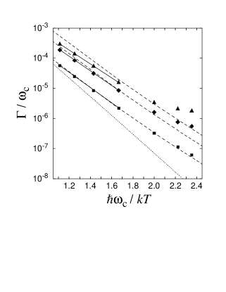FIG. 7.: Rates obtained in the low-temperature (activated) case for $\Lambda/\omega_{c}=30$. Results from summation over bridge diagrams for $\Delta/\omega_{c}=1$ (squares), $\Delta/\omega_{c}=2$ (diamonds), and $\Delta/\omega_{c}=3$ (triangles). The dashed lines indicate the Golden Rule rate for comparison ($\Delta/\omega_{c}=1$, $2$, and $3$, bottom to top). The classical nonadiabatic rate for $\Delta/\omega_{c}=1$ is given for comparison (dotted line). At high enough temperatures, Arrhenius-like behavior is observed, as indicated by the match between data and straight solid lines. Arrhenius behavior at low temperatures, with a rate that becomes much higher than its expected classical value.

We can put observations (a) and (b) on a more quantitative basis by separating the rate into an Arrhenius-like part and a temperature independent prefactor as

$$\Gamma=\nu\exp(-{F^{*}/kT})$$ (72)

Using (72) as an ansatz to fit our data between $kT/=0.6\,\hbar\omega_{c}$ and $kT/=\hbar\omega_{c}$, we can extract the $\Delta$-dependence of $\nu$ and $F^{*}$ separately, as shown in Fig. 8. The adiabaticity prefactor $\nu$ shows the expected transition from quadratic to saturation behavior, and the activation free energy $F^{*}$ shows approximately the expected linear decline.

Our diagrammatic theory reproduces the essential tenets of both the thermodynamic approach—the modification the reaction barrier through the electronic coupling—and of dynamical theories—the slowing of the reaction due to recrossing effects—in a unified description.

IV Summary and Conclusions

In this paper we have presented a novel dynamical approach to the theory of electron transfer reactions. The spin-boson model is used to represent electron transfer in 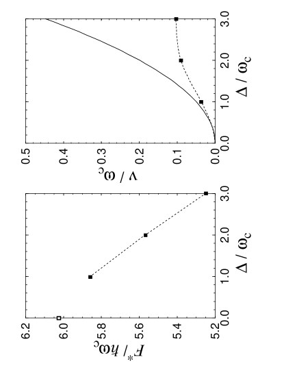                                                                                     FIG. 8.: (a) Activation free energy $F^{*}$ as a function of electronic overlap $\Delta$, using data from Fig. 7 between $kT=0.6\,\hbar\omega_{c}$ and $kT=\hbar\omega_{c}$. The open square at $\Delta=0$ denotes the Golden Rule value. (b) Adiabaticity prefactor $\nu$ from the same data. condensed-phase from a donor to an acceptor site. Relying on the established real-time path-integral representation of the spin-boson dynamics, we have for the first time rigorously deduced an exact rate expression in terms of the spin-boson parameters. In the nonadiabatic limit, our result reduces to the simpler NIBA description of spin-boson dynamics. Using the linked-cluster theorem, we have found a systematic way of summing up all corrections to the NIBA rate expression. Since we are using a dynamical treatment directly, our method is valid under rather weak assumptions and it is applicable in any parameter region that would yield a long-time limit of exponential decay of the reactant population.

We have demonstrated the relevance of our central results and the continued need for systematic groundwork for the electron transfer problem by pointing out significant discrepancies between results based on the linked-cluster sum (37) and previous approximate real-time or imaginary-time approaches. We have also shown the usefulness of our approach by presenting a resummation of the most important terms in the linked-cluster sum (42). This resummation imposes no approximation on terms up to order $\Delta^{4}$, and it retains a large, dominant class of diagrams for any order of the electronic or environmental coupling. Our results compare very favorably with published quantum Monte Carlo data and the results of a refined version of the resummation method.

The present approach provides a unified treatment of several characteristic features of adiabatic electron transfer which were reported earlier, but separately, using incompatible methods. Our results show two competing adiabatic effects. First, there is a rate reduction (compared to the nonadiabatic case), which has previously been described in terms of correlated recrossings of the Landau-Zener region. This effect is dominant at high temperatures. For low enough temperatures, one sees a transfer rate that is enhanced over the nonadiabatic result. This reflects the lowering of the reaction barrier by the electronic coupling and by nuclear tunneling. When higher demands on computational resources can be tolerated, our recursive resummation method may be extended to include larger classes of diagrams if higher accuracy is desired.