Monte Carlo Optimization of Trial Wave Functions in Quantum Mechanics and Statistical Mechanics

Abstract

This review covers applications of quantum Monte Carlo methods to quantum mechanical problems in the study of electronic and atomic structure, as well as applications to statistical mechanical problems both of static and dynamic nature. The common thread in all these applications is optimization of many-parameter trial states, which is done by minimization of the variance of the local energy or, more generally for arbitrary eigenvalue problems, minimization of the variance of the configurational eigenvalue.

I introduction

Many computational problems can be reduced to the computation of eigenvalues of operators. Examples of operators discussed in this paper are quantum mechanical Hamiltonians , transfer matrices, and stochastic (Markov) matrices. The applications discussed are: electronic eigenstates of atoms, and molecules; atomic eigenstates of clusters; critical point properties of classical statistical mechanical systems; and critical slowing-down of spin models.

In the review we assume that the reader is familiar with the Monte Carlo techniques in general. Readers who lack this familiarity may wish to consult the literature listed in Ref. [1].

Numerical computation of the eigenvalue spectrum of the full operator, or its approximate counterpart in a truncated representation of the state space, has been employed traditionally for this purpose, but more recently Monte Carlo eigenvalue methods have started to provide practical alternatives.

A particularly appealing feature of Monte Carlo eigenvalue methods is that the stochastic process can be used to estimate just the corrections to already sophisticated approximations. More specifically, these methods can be designed so that statistical errors vanish in the ideal case that the optimized trial states, which are pivotal in this approach, are exact eigenstates. In practice, one obviously cannot realize this ideal, but one can get close since there is much flexibility in the choice of trial functions, a flexibility which can be exploited to incorporate important physics in the approximation from the outset.

For the quantum mechanical applications, the flexibility of the functional form of the wave function is an important feature that can be exploited by the quantum Monte Carlo method and this distinguishes it from conventional quantum chemistry methods, such as Configuration Interaction (CI). It is possible to construct a compact and accurate wave function if its functional form incorporates the singularities of the true wave function, but CI, for example, uses an expansion in determinants of single-particle orbitals, which is slowly convergent because it cannot reproduce the cusps in the wave function at electron-electron coincidences[2]. In quantum Monte Carlo, however, functional forms can be used that are sufficiently flexible to have the correct singular behavior at the electron-nucleus, electron-electron and possibly higher-order particle coincidence points. This allows one to construct relatively compact wave functions with 50-100 free parameters and of quality comparable to CI wave functions with millions of determinants.

In applications, much effort is spent on the design and optimization of these trial states and this paper reviews various examples in which optimized trial states are employed, viz. the computation of eigenstates (mostly ground states) of atoms, molecules and van der Waals clusters, and the computation of critical exponents of static and dynamic equilibrium models with phase transitions in two and three dimensions. The examples discussed here are selected from work performed by the authors with various collaborators [3, 4, 5, 6, 7, 8, 9, 10, 11, 12, 13, 14] and this paper is not intended as a comprehensive review of the field.

II trial state optimization

First we consider the general principle [3, 4] of Monte Carlo optimization of a trial vector to approximate an eigenstate of an operator ${\rm\bf T}$. In principle, the method is applicable to an arbitrary discrete state anywhere in the spectrum, but in practice it is used for eigenvalues at the top or bottom of the spectral sector compatible with the desired symmetry, unless one starts out with an estimate of the energy of an excited state, that is accurate relative to the gaps separating it from neighboring eigenvalues. More specifically, as mentioned, the applications to be discussed will be drawn from quantum mechanics, and static and dynamic equilibrium statistical mechanics.

If the operator ${\rm\bf T}$ is a quantum mechanical Hamiltonian $\cal H,$ the trial state, in most cases discussed below, is an approximation for the fermionic ground state in the case of atoms and molecules, or the bosonic ground state in the case of the van der Waals clusters. In the statistical mechanics statics case, ${\rm\bf T}$ is the transfer matrix , and here the state of interest is the dominant eigenstate, the state with the eigenvalue of largest magnitude. In the application to stochastic processes satisfying detailed balance, the largest eigenvalue is unity and the associated eigenstate is the Boltzmann distribution. In this case, one is interested in the dominant non-trivial state, i.e., the state with the second largest eigenvalue, which in the case discussed below is the dominant antisymmetric state.

For simplicity of presentation we assume that the operator ${\rm\bf T}$ is hermitian. In practice, the method is applied to non-hermitian operators as well, since transfer matrices are used for systems with helical boundary conditions. Owing to the helicity, the transfer matrices have the property

$${\rm\bf T}^{\dagger}={\rm\bf R}{\rm\bf T}{\rm\bf R},$$ (1)

where ${\rm\bf R}$ is a reflection operator, i.e., ${\rm\bf R}^{2}=\openone$. This property implies that a simple relation exists between left and right eigenstates, which is usually not the case for non-hermitian operators. As a consequence, the discussion below can be immediately generalized to transfer matrices, but to simplify the presentation we omit further technical details.

Consider a trial state $|{{\psi_{\/\rm T}}}\rangle$ depending on a set of optimization parameters. Optimal values for the parameters can, in principle, be found by minimization of the quantity

$$\sigma^{2}={\langle{{\psi_{\/\rm T}}}|({\rm\bf T}-\langle{\rm\bf T}\rangle)^{2}|{{\psi_{\/\rm T}}}\rangle\over\langle{{\psi_{\/\rm T}}}|{{\psi_{\/\rm T}}}\rangle},$$ (2)

where

$$\langle{\rm\bf T}\rangle={\langle{{\psi_{\/\rm T}}}|{\rm\bf T}|{{\psi_{\/\rm T}}}\rangle\over\langle{{\psi_{\/\rm T}}}|{{\psi_{\/\rm T}}}\rangle}.$$ (3)

Note that $\sigma^{2}$ assumes its minimum value, zero, for any eigenstate of the operator ${\rm\bf T}$.

In practical applications, the variance $\sigma^{2}$ cannot be evaluated directly, and a Monte Carlo estimate is used instead. This can be done by generating a sample ${\cal S}$ of configurations $s$ drawn from a suitable relative probability distribution $\langle{s}|{\gamma}\rangle^{2}$, as given, for example, by a trial state defined by initial guesses for the optimization parameters. Given this sample ${\cal S}$, one can evaluate

$$\sigma^{2}\approx{\sum_{s\epsilon{\cal S}}[t(s)-\bar{t}\,]^{2}w_{s}^{2}\over\sum_{s\epsilon{\cal S}}w_{s}^{2}}.$$ (4)

Here the $w_{s}$ are weights defined by $w_{s}={\langle{s}|{{\psi_{\/\rm T}}}\rangle/\langle{s}|{\gamma}\rangle}$ and $\bar{t}$ is the corresponding weighted sample average of the configurational eigenvalue, which is called the local energy in real-space quantum Monte Carlo applications,

$$t(s)={\langle{s}|{\rm\bf T}|{{\psi_{\/\rm T}}}\rangle\over\langle{s}|{{\psi_{\/\rm T}}}\rangle}.$$ (5)

To avoid spurious minima of $\sigma^{2}$, which may arise when very few configurations acquire most of the weight, it is advisable in practice to evaluate the expressions in Eqs. (4) and (5) using redefined weights $w_{s}$ that are bounded from above.

For this optimization algorithm to be practical, the configurational eigenvalue $t(s)$ has to be computable without explicit summation or integration over all states of a complete set inserted between ${\rm\bf T}$ and $|{{\psi_{\/\rm T}}}\rangle$, a condition which is satisfied, e.g., if ${\rm\bf T}$ is sparse or near-local. In this case, optimal parameters can be found efficiently with a modified version [15] of the Levenberg-Marquardt algorithm, designed to minimize a sum of squares, such as the expression given in Eq. (4).

The crux of the method is that this procedure is applied to a fixed, small sample, which works efficiently as long as the sample is a good representation of $|{{\psi_{\/\rm T}}}\rangle$, the trial state defined by the current parameter estimates. How well the sample generated by means of the state $|{\gamma}\rangle$ represents the state $|{{\psi_{\/\rm T}}}\rangle$, can be measured by the overlap

$$c={\langle{{\psi_{\/\rm T}}}|{\gamma}\rangle\over\sqrt{\langle{\gamma}|{\gamma}\rangle\langle{{\psi_{\/\rm T}}}|{{\psi_{\/\rm T}}}\rangle}},$$ (6)

or in more practical terms

$$c^{2}\approx{(\sum_{s\epsilon{\cal S}}w_{s})^{2}\over|S|\sum_{s\epsilon{\cal S}}w_{s}^{2}}.$$ (7)

Usually, one chooses for $|{\gamma}\rangle$ the best available approximation to the optimized trial state, in which case Eq. (6) can be used irrespective of the signs of the weights $w_{s}$, which will be predominantly of one sign. In some cases, however, it is convenient to draw a sample from a state (almost) orthogonal to $|{{\psi_{\/\rm T}}}\rangle$. For example, in the case of the optimization of the trial state for the second-largest eigenstate of the Markov matrix , discussed in more detail in Section V C, it is convenient to sample states from the Boltzmann distribution, a state of even symmetry, while the desired state is odd. Whether this process yields a representative sample can be estimated if $w_{s}$ is replaced by $|w_{s}|$ in Eq. (7). In any event, whenever the overlap becomes too small, a new sample has to be generated, e.g., from the current, improved trial state, and this process is iterated until it converges.

The above procedure deviates from the standard Rayleigh-Ritz variational approach of optimizing the Rayleigh quotient defined in Eq. (3). As mentioned above, minimization of the variance of the configurational eigenvalue has the advantage of being applicable also to excited states. Perhaps more important in a Monte Carlo context is that minimization of the $\sigma^{2}$ is more stable numerically. That is, although the exact Rayleigh quotient is bounded by the extremal eigenvalues, this property no longer holds for the approximation involving sums over a finite sample of states, in particular because this sample is necessarily extremely sparse when one is dealing with high-dimensional problems, which is the case for most problems of practical interest. Since one is varying many parameters, the estimate of the Rayleigh quotient in terms of finite sums can easily become dominated by a single state, as can be seen by considering the Monte Carlo estimate of the Rayleigh quotient used in the minimization, viz.

$$\langle{\rm\bf T}\rangle\approx{\sum_{s\epsilon{\cal S}}t(s)w_{s}^{2}\over\sum_{s\epsilon{\cal S}}w_{s}^{2}}.$$ (8)

an expression in which $t(s)$ is not necessarily bounded from below for all parameter values. The Monte Carlo estimate of $\sigma^{2}$, on the other hand, although approximate, remains a sum of squares and cannot be made artificially small as long as more states effectively contribute to the sum than there are parameters. An additional computational advantage is that there are better methods, such as the Levenberg-Marquardt algorithm mentioned above[15], to optimize a sum of squares than to optimize a general function.

A possible source of instability of the above algorithm is the fact that $\bar{t}$ can assume misleading values. For instance, in the optimization of a quantum mechanical bound state, one can encounter a sample and parameter values such that only states in the tail of the wave function carry considerable weight. This can produce an artificially small estimate of the variance, resulting from the fact that frequently only a few parameters have to be adjusted to obtain a local energy that is fairly constant over the contributing part of such sample. Simple variations of the object function can help cure this problem. First of all, one can replace the weighted sample average $\bar{t}$ in Eq. (4) by a constant estimate of the eigenvalue [3, 4]. In this way, one can maintain focus on the ground state and obtain an object function that interpolates between minimization of the variance and minimization of the Rayleigh quotient by choosing a fixed value for $\bar{t}$ below the true eigenvalue (or above in case one is interested in the largest eigenvalue). An alternative method [11] of accomplishing this is to use as the object function $\sigma^{2}/\bar{t}\,^{2}$.

III Atoms and Molecules

A Trial wave functions

Trial wave functions commonly used in quantum Monte Carlo applications to problems in electronic structure are a sum of products of up- and down-spin determinants of single-particle orbitals multiplied by a Jastrow factor

$$\Psi=J\sum_{n}d_{n}D^{\uparrow}_{n}D^{\downarrow}_{n}.$$ (9)

$D^{\uparrow}_{n}$ and $D^{\downarrow}_{n}$ are the Slater determinants of single particle orbitals for the up and down electrons respectively. The orbitals are linear combinations of products of Slater basis functions and spherical harmonics centered at the nuclei.

Filippi and Umrigar use a Feenberg or generalized Jastrow factor $J$, which is a modification of the form introduced by Umrigar et al.[3, 4, 16] to account explicitly for correlations between a nucleus and two electrons. This form is a generalization of the Boys and Handy [17] form. Subsequently, employing wave functions based on back-flow arguments, Schmidt and Moskowitz [18, 19] attempted to reduce the number of parameters in the wave functions used by Umrigar et al..

The generalized Jastrow factor is written as a product of factors describing two- and three-body interactions. The notation is as follows: electrons are labeled by $i$ and $j$, while $\alpha$ labels the nuclei. The electron-nucleus correlation is described by $A_{\alpha i}$, the electron-electron correlation $B_{ij}$; and $C_{\alpha ij}$ gives the correlation of two electrons and a nucleus. Thus, the following form is obtained

$$J=\prod_{\alpha,i}\,\exp{A_{\alpha i}}\;\;\prod_{i,j}\,\exp{B_{ij}}\;\;\prod_{\alpha,i,j}\,\exp{C_{\alpha ij}}.$$ (10)

The electron-nucleus contribution $A_{\alpha i}$ could in principle be omitted from the Jastrow factor, provided that a sufficiently large single-particle basis is used in the determinantal factor of the wave function. Three-electron correlations are not included in the Jastrow factor, since the proximity of more than two electrons is rendered unlikely by the exclusion principle, incorporated in the Slater determinant. The importance of three-electron and higher-order terms is discussed in [20].

The exponents $A_{\alpha i}$, $B_{ij}$, and $C_{\alpha ij}$ of the Jastrow factor are written as functions of the inter-electronic distances $r_{ij}$ and electron-nucleus distances $r_{i\alpha}$. These exponents are chosen to be either polynomials or rational functions expanded in scaled variables $\hat{r}_{ij}$ and $\hat{r}_{i\alpha}$, where $\hat{r}=[1-\exp(-\kappa r)]/\kappa$, which at large inter-particle distances prevents domination of these polynomials by their highest-order terms. Typically, either a 5^th order polynomial or a 4^th order rational function is used. Increasing the order beyond this does not yield a significant improvement in the wave function (except in the case of the two-electron systems) since the bottleneck is due to the missing higher body-order correlations in the Jastrow and the determinantal parts of the wave function. In addition to these analytic terms, $C_{\alpha ij}$ contains non-analytic terms that suppress the dependence of the local energy on the shape of the triangle formed by two electrons and a nucleus for configurations in which two electrons simultaneously approach the nucleus. The Fock expansion motivates the detailed form of these terms; we refer to Refs. [14] and [21] for details.

To guarantee that the local energy remains finite when two electrons, or an electron and a nucleus approach each other, cusp conditions are imposed on the wave function. The resulting algebraic relations among the variational parameters of the wave function significantly reduce the number of free parameters.

To summarize, the parameters are of several different types: a) the exponents of the Slater basis functions; b) the linear coefficients used to construct orbitals from the basis functions; c) the linear coefficients in the combination of determinants; d) the exponent $\kappa$ used to define the scaled inter-particle distances; and e) expansion coefficients of the polynomial or rational functions in the Jastrow factor [cf. Eq. (10)]. The last set accounts for most of the parameters, the total number being on the order of 60, even after taking into account the reduction in the number of free parameters resulting from the imposition of symmetry and cusp-condition constraints. Although this is a substantial number, it is orders of magnitude smaller than the number of coefficients required in configuration interaction wave functions of similar accuracy. The freedom quantum Monte Carlo methods provide in the choice of the form of the trial wave functions pays off!

Optimization of a trial wave function of the complexity described above is best performed in a step-wise fashion. The starting point is an approximate Hartree-Fock wave function composed of the minimum number of determinants of the lowest single particle orbitals necessary to obtain a state of the desired symmetry. This Hartree-Fock wave function is multiplied by the Jastrow factor described above, whereupon all parameters are optimized. Continuing from this intermediate trial function, multi-determinantal trial functions can be constructed by adding configuration state functions corresponding to single and double excitations from the Hartree-Fock configuration. To select these additional configurations, a Multiconfiguration Self-Consistent Field wave function is obtained with a standard quantum chemistry package and the configurations with large weight are added to the best previous wave function. Finally, all parameters are re-optimized simultaneously.

B Results for atoms and molecules

Accurate wave functions and energies for small atoms and ions[3, 4, 16] and small molecules[14] were calculated. Three measures were used to judge the quality of the wave functions: the percentages of the correlation energy recovered in variational and in diffusion Monte Carlo , and the root-mean-square fluctuation of the local energy $\sigma_{\rm VMC}$ obtained by variational Monte Carlo. The results are contained in Table I, which also contains the variational and diffusion Monte Carlo energy estimates $E_{\rm VMC}$ and $E_{\rm DMC}$. Some of the values of $E_{\rm VMC}$ and $\sigma_{\rm VMC}$ are better than those presented in earlier papers, the improvements being both the result of small modifications that were made to the form of the wave functions and of further optimization. We note that the results for the two-electron atoms and ions are exceptionally accurate. This is because the Jastrow factor includes all-body correlations, i.e., the correlations of both electrons and the nucleus. Note however that simply increasing the order of the polynomials or rational functions in the Jastrow factor yields almost arbitrarily accurate wave functions only for node-less ground states or states in which the nodal surface is determined by symmetry alone.

Included in Table I are the energies of the 1³S He and the 2³S He excited states. The 1³S He state is the lowest state of that symmetry but the 2³S He is not. The accurate energy obtained for the 2³S He illustrates that the variance minimization method can be used to obtain accurate wave functions not only for the lowest states of a given symmetry, but for true excited states as well, provided that the energy gap between the desired state and neighboring states of the same symmetry is larger than the fluctuations of the local energy for the desired trial state. The energies obtained for all the two-electron states from variational Monte Carlo  is so good that it is not necessary to perform diffusion Monte Carlo  calculations.

The energies obtained for the four- and ten-electron systems are also very accurate though of course not of accuracy comparable to those for the two-electron systems. We note that for the four-electron systems it is essential to include the low-lying second configuration state function, coming from the 2s${}^{2}\to$2p² excitation, in order to obtain an accurate energy.

TABLE I.: Total energies for atoms and ions. $E^{\rm VMC}_{c}$ and $E^{\rm DMC}_{c}$ are the percentages of correlation energy recovered in variational Monte Carlo  and diffusion Monte Carlo. $\sigma_{\rm VMC}$ is the root-mean-square fluctuation of the local energy. The numbers in parentheses are the statistical errors in the last digit. The second column lists the number of configuration state functions (CSF) and the number of determinants ($D$) in the wave function. Energies are in Hartree atomic units. The percentages were calculated using the Hartree Fock and virtually exact energies from the references cited. (Taken from Ref. [3, 4, 16] and updated.)

atom/ion	CSF,D	$E_{\rm VMC}$	$E_{\rm DMC}$	$E^{\rm VMC}_{c}(\%)$	$E^{\rm DMC}_{c}(\%)$	$\sigma_{\rm VMC}$
11S H-	1,1	$-0.527,750,6(1)$		$99.9990(2)\cite[cite]{[\@@bibref{Number}{Fisher,Freund}{}{}]}$		$0.0007$
11S He	1,1	$-2.903,724,4(1)$		$100.0000(2)\cite[cite]{[\@@bibref{Number}{Fisher,Freund}{}{}]}$		$0.0007$
13S He	1,1	$-2.175,229,3(1)$		$100.00(1)\cite[cite]{[\@@bibref{Number}{Fisher,Drake}{}{}]}$		$0.0003$
23S He	1,1	$-2.068,688,7(1)$		$99.80(5)\cite[cite]{[\@@bibref{Number}{Fisher,Drake}{}{}]}$		$0.0011$
11S Be2+	1,1	$-13.655,566,2(1)$		$100.0000(2)\cite[cite]{[\@@bibref{Number}{Fisher,Freund}{}{}]}$		$0.0014$
11S Li-	2,4	$-7.500,30(1)$	$-7.500,69(1)$	$99.45(1)\cite[cite]{[\@@bibref{Number}{Fisher,Fisher93}{}{}]}$	$99.91(1)$	$0.044$
11S Be	2,4	$-14.666,65(1)$	$-14.667,19(1)$	$99.25(1)\cite[cite]{[\@@bibref{Number}{Fisher,Davidson}{}{}]}$	$99.82(1)$	$0.084$
11S Ne	1,1	$-128.901,1(1)$	$-128.923,6(2)$	$90.56(2)\cite[cite]{[\@@bibref{Number}{Fisher,Chakravor}{}{}]}$	$96.32(4)$	$0.89$

TABLE II.: Total energy of Li₂ for increasing number of configuration state functions (CSF). The configurations are listed without the doubly occupied core molecular orbital $1\sigma_{\rm g}$. $E_{\rm VMC}$ and $E_{\rm DMC}$ are estimates of the energy obtained by variational Monte Carlo  and fixed node diffusion Monte Carlo; $E^{\rm VMC}_{c}$ and $E^{\rm DMC}_{c}$ are the respective percentages of correlation energy. $\sigma_{\rm VMC}$ is the root-mean-square fluctuation of the local energy of the optimized trial state. The numbers in parentheses are the statistical errors in the last digit. Energies are in Hartree atomic units. (Taken from Ref. [14].)

CSF/D	additional CSF	$E_{\rm VMC}$	$E_{\rm DMC}$	$E_{c}^{\rm VMC}(\%)$	$E_{c}^{\rm DMC}(\%)$	$\sigma_{\rm VMC}$
1,1	$2\sigma_{\rm g}^{2}$	$-14.97343(7)$	$-14.9911(1)$	$82.26(5)$	$96.5(1)$	$0.112$
2,1	$2\sigma_{\rm u}^{2}$	$-14.97745(6)$	$-14.9909(1)$	$85.51(4)$	$96.4(1)$	$0.098$
3,4	$1\pi_{\rm ux}^{2}+1\pi_{\rm uy}^{2}$	$-14.98404(5)$	$-14.9923(1)$	$90.83(4)$	$97.5(1)$	$0.086$
4,5	$3\sigma_{\rm g}^{2}$	$-14.98850(4)$	$-14.9938(1)$	$94.43(4)$	$98.7(1)$	$0.086$

TABLE III.: Total energies for the best single- and multi-configuration wave functions. As in Table II, $E^{\rm VMC}_{c}$ and $E^{\rm DMC}_{c}$ are the percentages of correlation energy recovered in variational Monte Carlo  and diffusion Monte Carlo. $\sigma_{\rm VMC}$ is the root-mean-square fluctuation of the local energy of the optimized trial state. The numbers in parentheses are the statistical errors in the last digit. The second column lists the number of configuration state functions (CSF) and the number of different determinants ($D$) in the wave function. Energies are in Hartree atomic units. (Taken from Ref. [14].)

molecule	CSF,D	$E_{\rm VMC}$	$E_{\rm DMC}$	$E^{\rm VMC}_{c}(\%)$	$E^{\rm DMC}_{c}(\%)$	$\sigma_{\rm VMC}$
Li2	1,1	$-14.97343(7)$	$-14.9911(1)$	$82.26(5)$	$96.5(1)$	$0.112$
	4,5	$-14.98850(4)$	$-14.9938(1)$	$94.43(4)$	$98.7(1)$	$0.086$
Be2	1,1	$-29.2782(1)$	$-29.3176(4)$	$70.70(7)$	$89.8(2)$	$0.242$
	5,16	$-29.3129(1)$	$-29.3301(2)$	$87.56(6)$	$95.9(1)$	$0.215$
B2	1,1	$-49.3115(3)$	$-49.3778(8)$	$68.06(8)$	$88.5(2)$	$0.432$
	6,11	$-49.3602(2)$	$-49.3979(6)$	$83.10(7)$	$94.7(2)$	$0.408$
C2	1,1	$-75.7567(5)$	$-75.8613(8)$	$67.82(9)$	$88.1(2)$	$0.707$
	4,16	$-75.8282(4)$	$-75.8901(7)$	$81.66(7)$	$93.6(1)$	$0.641$
N2	1,1	$-109.3756(6)$	$-109.487(1)$	$69.7(1)$	$89.9(2)$	$0.935$
	4,17	$-109.4376(5)$	$-109.505(1)$	$80.94(8)$	$93.1(2)$	$0.863$
O2	1,1	$-150.1507(6)$	$-150.268(1)$	$73.4(1)$	$91.0(2)$	$1.09$
	4,7	$-150.1885(5)$	$-150.277(1)$	$79.08(8)$	$92.5(2)$	$1.05$
F2	1,1	$-199.3647(7)$	$-199.478(2)$	$78.26(9)$	$93.2(2)$	$1.23$
	2,2	$-199.4101(6)$	$-199.487(1)$	$84.23(8)$	$94.3(1)$	$1.19$

FIG. 1.: Percentage of correlation energy in variational Monte Carlo  (upper plot) and diffusion Monte Carlo  (middle plot) and root-mean-square fluctuation $\sigma_{\rm VMC}$ (lower plot) with one-configuration (full circle) and multi-configuration (empty circle) wave functions. (Taken from Ref. [14].)

Filippi and Umrigar computed both single and multi-configuration wave functions for the first-row homo-nuclear diatomic molecules, Li₂, Be₂, B₂, C₂, N₂, O₂ and F₂ with trial wave functions optimized at the experimental bond length. Results illustrating the effect of including additional configuration state functions are shown in Table II for Li₂. As configurations are added, there is an improvement in all three quantities of interest, $\sigma_{\rm VMC}$, E_VMC and E_DMC (except that the one- and two-configuration E_DMC and the three- and four-configuration $\sigma_{\rm VMC}$ are the same within the statistical errors), but the best result achieved for Li₂ is not as good as for the two-configuration Be wave function. In the case of Be there is a single low-lying configuration that mixes in strongly, whereas for Li₂ there are several configurations that make smaller contributions.

Table III shows the total energies obtained in variational Monte Carlo  and diffusion Monte Carlo  and $\sigma_{\rm VMC}$ obtained with single-determinant and multi-determinant wave functions. The percentage of correlation energy recovered is plotted in Figure 1. It ranges from 68-82% for single-configuration and 79-94% for multi-configuration wave functions in variational Monte Carlo. The corresponding numbers are 88.1-96.5% and 92.5-98.7% in diffusion Monte Carlo. For the single-configuration wave functions, the smallest percentage of correlation energy recovered is not for the heaviest molecules but rather for the molecules in the middle of the row owing to the strong multi-configurational nature of their true ground state. For the multi-configuration wave functions, the smallest percentage moves more to the right of the row where, possibly, excitations to the next shell become important. Since the wave functions are obtained by non-linear optimization, it is possible to get stuck in a local minimum. From the shape of the curves it seems likely that this is in fact the case for O₂. There is considerable resemblance in the shapes of the variational Monte Carlo and diffusion Monte Carlo curves and the multi-configuration energies are consistently better than their single-configuration counterparts. Therefore, it is clear that when more configurations are added to the HF one, not only do $\sigma_{\rm VMC}$ and E_VMC improve but there also is an improvement in the shape of the nodal surface, flaws in which limit the accuracy of the fixed-node diffusion Monte Carlo energies.

These results shed some light on the question how the computational complexity of quantum Monte Carlo scales with atomic number $Z$. In going from Li₂ to F₂, the root-mean-square fluctuation of the local energy, $\sigma_{\rm VMC}$, increases by more than a factor of ten for both the single and the multi-configuration wave functions. The dependence of $\sigma_{\rm VMC}$ on atomic number $Z$ appears to be considerably faster than linear for small $Z$ but slower than linear for large $Z$. This factor should be taken into account in figuring the scaling of the computational cost. In order to estimate this scaling, it is necessary to have a systematic study of several molecules. It would in fact be useful to also have results on some second-row homo-nuclear diatomic molecules.

IV Bosonic van der Waals clusters

A Introduction

As a next example, we discuss bosonic van der Waals clusters. Again, in this case most of the work focuses on trial wave functions for the ground state.

Mushinski et al. [9, 11] study clusters consisting of $N$ Lennard-Jones atoms interacting via the pair potential $v(r)=4\epsilon[(r/\sigma)^{-12}-(r/\sigma)^{-6}]$. In reduced units, the potential takes the form $v(r)=r^{-12}-2r^{-6}$ and the only independent parameter in the Schrödinger equation is the reduced inverse mass $m^{-1}$, which is proportional to the square of the de Boer parameter, $h/\sigma\sqrt{m\epsilon}$, a dimensionless quantity measuring the relative importance of quantum mechanical effects.

Constructing accurate trial wave functions is particularly challenging for large values of the de Boer parameter, and part of the work to be discussed here deals with clusters in the extreme case, viz. the unbinding limit, where the zero-point energy is sufficiently strong to destroy the bound-state nature of the ground state of a cluster. The corresponding value of the de Boer parameter plays the role of a critical point, and in fact the unbinding transition has many features in common with a critical wetting transition [28]. For bosonic clusters, the unbinding is of theoretical interest, but the transition is not experimentally observable. That is, in the first place, the critical de Boer parameter is an increasing function of the geometric size of the cluster, or in other words, the binding energy per atom increases with the size of the cluster. Secondly, for the bosonic atom with largest de Boer parameter, ⁴He, the dimer is believed to have in a bound state, so that one expects the same for clusters of all sizes. For fermion clusters, however, it is estimated that ³He clusters only have bound states for more than 30 atoms[29]. From this point of view the boson computations are to be viewed as a test case for the experimentally more interesting fermion case.

Simple arguments[11] applied to this unbinding transition predict the way in which the energy vanishes as the de Boer parameter approaches its critical value, and the nature of the divergence of the size of the clusters. More specifically, the following critical behavior is expected for the ground state energy $E_{0}$ and the average size $\langle r\rangle$ (as defined below) of the cluster

$$E_{0} \sim (\Delta m)^{2},$$ (11)

$$\langle r\rangle \sim (\Delta m)^{-1},$$ (12)

for ${m\downarrow m_{\rm c}}$ where $\Delta m=m-m_{\rm c}$ with $m_{\rm c}$ the critical value of the dimensionless mass. Results corroborating these predictions will be discussed. In addition, this section discusses a graphical method of inspecting the quality of the trial wave functions, in particular to identify regions that contribute excessively to the variance of the local energy.

B Cluster trial functions

The construction of the trial wave functions for clusters closely parallels the discussion above in section III, i.e., a trial wave function for the ground state of a bosonic cluster should be invariant under translation, rotation and particle permutation. The first two of these requirements can be satisfied by choosing as coordinates the inter-atomic distances $r_{ij},\ 1\leq i<j\leq N$. The third condition, particle exchange symmetry, then can be imposed explicitly by considering only functions that are invariant under the $N!$ permutations of the indices of the $r_{ij}$. The technical problems associated with this permutation symmetry can be dealt with efficiently by employing an approach based on the theory of algebraic invariants and we refer to Ref. [9] for details.

In addition to having to satisfy these symmetry restrictions, the ground state trial function has to be strictly positive. In principle, $n$-body correlations with all $n\leq N$, should be incorporated in the trial wave function, but these many-body effects are expected to become progressively less important as $n$ increases. Positivity and many-body correlations suggest that the trial function be written as

$$\log{\psi_{\/\rm T}}=\sum_{(i,j)}u^{(2)}(r_{ij})+\sum_{(i,j,k)}u^{(3)}(r_{ij},~{}r_{jk},~{}r_{ki})+\cdots+\sum_{(i_{1},\dots,i_{N})}u^{(N)}(r_{i_{1}i_{2}},\dots),$$ (13)

where the $u^{(n)}$ are real-valued, $n$-body functions.

The design of trial wave functions, described in detail in Ref. [9], used the procedure developed by Umrigar et al. [3, 4]. That is, the trial functions satisfy boundary conditions associated with (a) the collision of two atoms and (b) one atom going off to infinity. The behavior of the wave function for the most likely configurations, which involve intermediate distances and require most of the variational freedom of the trial wave functions, is described by expanding the $u^{(n)}$ in polynomials of variables $\hat{r}_{ij}=\hat{r}(r_{ij})$, where $\hat{r}$ is an optimizable function that approaches a constant for $r\to\infty$. Note that $u^{(2)}$ is exceptional in that in addition to these polynomial terms, it has terms dictated by the short-distance and long-distance boundary conditions.

Wave functions of this type can be used to study the importance of many-body effects for the quality of the trial wave function. The exact ground state energy $E_{0}$ and its variational estimate $\tilde{E}_{0}$ satisfy the inequality

$$\tilde{E}_{0}-\sigma\leq E_{0}\leq\tilde{E}_{0}.$$ (14)

This suggests that the quality of the trial wave function ${\psi_{\/\rm T}}$ be measured by

$$Q=-\log_{10}{\sigma\over|E_{0}|}.$$ (15)

The limit $Q\to\infty$ corresponds to an exact solution of the time-independent Schrödinger equation. The quantity $Q$ is a conservative measure of the accuracy of the wave function since in fact, there exists a tighter bound, linear in $\sigma^{2}$ rather than $\sigma$; we refer to Refs. [9] and [11] for details.

With these wave functions containing an arbitrary number of many-body correlations Mushinski and Nightingale [9] address the question how the quality of the trial wave function improves as $n$-body terms with progressively larger values of $n$ are included. Figures IV B through IV B display results for Ar clusters of sizes three, four, and five. The estimate $Q$ of the quality of the wave functions is plotted versus the power $P$ of the polynomials used in the expansion of Eq. (13) for different values of $n$. The bottom curve, starting at $P=1$, is for the case in which only two-body interactions are present ($n=2$). As shown, the quality levels off at a fixed value of $Q$ with increasing $P$, an indication that the absence of three-body terms is the dominant source of variance of the local energy. In the next curve segment, three-body terms are added ($n=3$). Here $P$ is redefined to denote the order of the three-body polynomial, which starts at $P=2$; in the second curve segment the order of the polynomial that describes two-body effects is kept constant at the highest $P$-value used in the previous segment of the curve. This process is repeated for $n$-body terms with increasing $n$, until finally the complete $N$-body polynomial for the $N$-atom cluster is included in the trial function. At this point, the quality starts to go up roughly linearly with the order of the polynomial. Similar results were obtained for systems made of lighter atoms[9]. Here we only note that the order $P$ of the four-body polynomials is not sufficiently high in any of the figures for the quality to have leveled off, as ultimately it must for five-atom clusters.

Figures IV B, IV B, and IV B are plots of the quality $Q$ vs. the power $P$ for each type and size of cluster for optimized wave functions constructed of the full many-body polynomials. An interesting feature of these plots is that the $Q$ vs. $P$ curves for three- and four-atom ($N=3,4$) clusters almost coincide but that they are distinct from the curves for $N=2$ and $N=5$. The $N=2$ clusters are unique in that the short-distance divergences in the local energy have been fully removed, while also the large-distance asymptotic properties of the trial function is superior in this case. Apart from this, the effect probably is geometric in nature: only for sizes $N\leq 4$ are clusters fully symmetric in the classical configuration of minimum energy and are all atoms are at the bottom of the individual pair potentials. The same is true for $N=5$ in four dimensions and indeed the accuracy of the wave functions in that case is comparable to that in the $N=3$ and $N=4$ cases in three dimensions.

Finally, Table IV contains ground state energies obtained with the help of the optimized trial functions discussed above.

FIG. 2.: Quality $Q$, a measure of the accuracy of the optimized trial function as defined in Eq. (15), as a function of the power $P$ of two- and three-body polynomials, labeled by $n$, for $\mbox{Ar}_{3}$. From Ref. [9].

FIG. 3.: Quality $Q$, a measure of the accuracy of the optimized trial function as defined in Eq. (15), as a function of the power $P$ of two- , three- and four-body polynomials, labeled by $n$, for $\mbox{Ar}_{4}$. (Taken from Ref. [9].)

FIG. 4.: Quality $Q$, a measure of the accuracy of the optimized trial function as defined in Eq. (15), as a function of the power $P$ of two-, three-, four- and five-body polynomials, labeled by $n$, for $\mbox{Ar}_{5}$. (Taken from Ref. [9].)

FIG. 5.: Quality $Q$, a measure of the accuracy of the optimized trial function as defined in Eq. (15), as a function of power $P$ of the complete $N$-body polynomial for argon clusters of sizes two through five. The curve for Ar₂ levels off because of noisy behavior of the numerical derivatives used in the computations. Apparent erratic behavior of the Ar₅ curve is presumably due to occasional suboptimal parameter choices for the trial wave function. (Taken from Ref. [9].)

FIG. 6.: Quality $Q$, a measure of the accuracy of the optimized trial function as defined in Eq. (15), as a function of power $P$ of the complete $N$-body polynomial for neon clusters of sizes two through five. (Taken from Ref. [9].)

FIG. 7.: Quality $Q$, a measure of the accuracy of the optimized trial function as defined in Eq. (15), as a function of power $P$ of the complete $N$-body polynomial for clusters of sizes two through five; the clusters consist of hypothetical “${1\over 2}$-Ne” atoms with a reduced mass equal to half that of neon . (Taken from Ref. [9].)

C Visualization of flaws of the trial wave function

In the process of construction of the trial functions, it is important to know what regions of configuration space contribute most to the variance $\sigma^{2}$, as defined in Eq. (2). For instance, it is useful to know if the quality of the wave function is limited by poorly satisfied boundary conditions (either at infinity or when two particles get close) or if the quality can be improved by adding more variational parameters. A wave function subjected to the optimization procedure described in Section II might have too much variational freedom relative to the size of the sample over which it is optimized. This might show up in the form of unphysical peaks, which might remain invisible in the variance of the local energy estimated from the relatively small samples used to optimize the trial function.

To help answer such questions, Meierovich et al.[11] made density plots of the local error, the deviation of the local energy from its average and, as an illustration, they discuss a five-atom cluster. In fact, it is useful to superimpose color density plots of both the wave function and the local error, which contain more information than can be reproduced by the grey-scale plots reproduced in this paper. See Ref. [30] for the color graphics.

Obviously, the fact that the ground state wave function depends on $3N-6$ independent coordinates, seriously limits any graphical approach. For five-atom clusters the following planar cut through configuration space is informative: four atoms are fixed at the vertices of a regular tetrahedron, while the fifth particle is located in a plane that contains two of these vertices and bisects the edge connecting the two remaining atoms.

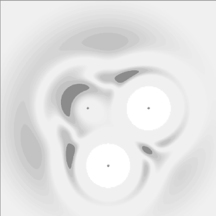
FIG. 8.: Left: Density plot of the “local error” in the geometry described in the text. The two dots in the lower right-hand corner are the two in-plane vertices of the tetrahedron; the one in the upper left corner is the projection of the two out-of-plane vertices. The length of the tetrahedron edges is 1.3 and $m^{-1}=0.16$. The darker the region, the more it contributes to $\sigma^{2}$. Note that the dark region in the lower right is a cut through the banana-shaped dark region in the upper left. The regions of the largest local error are the two symmetrically located regions of collision of four atoms. White lines are are cuts through nodal surfaces of the local error and have no physical significance.
Right: Density plot of $|\psi_{T}|^{2}$ as a function of the position of the fifth particle in same geometry Dark regions correspond to high probability density. Note that the regions with the largest local error are contained in the region where the wave function becomes small because of repulsive potential at short range. (Taken from Ref. [11].)

Figures 8 strongly suggest which regions of configuration space contribute most to $\sigma^{2}$. The density plots should be interpreted according to the following convention: zero intensity (white) corresponds to a minimum, while full intensity (black) corresponds to a maximum of the plotted function. The picture on the left in Figure 8 represents the density plot of the weighted local error, defined as $|({\cal E}-E_{\rm T})\psi_{\/\rm T}|$, as a function of the position of the fifth, wandering atom. [Note that the local energy ${\cal E}$ is defined by Eq. (5) with ${\rm\bf T}$ replaced by the Hamiltonian. ] The picture on the right in Figure 8 shows the dependence of $\psi_{\/\rm T}^{2}$, on the position of the fifth atom while the other four atoms are fixed in the geometry mentioned above.

The conclusion drawn from inspection of the density plots is that the trial function fails particularly in regions where more than two atoms collide and we see that, of these, the four-body collisions are worst at least in a local sense.

TABLE IV.: $E_{\rm T}$ and $E_{0}$, variational and diffusion Monte Carlo estimates of the ground state energies of noble gases Ar and Ne, and hypothetical “${1\over 2}$-Ne” for clusters of $N$ atoms, from Refs. [9] and [11]. Standard errors in the last digits are given in parentheses. The relative numerical error of these estimates is on the order of $10^{-7}$, which in some cases exceeds the statistical error. (Taken from Ref. [11].)

	$N$	$E_{\rm T}$	$E_{0}$
Ar	3	$-2.553335364(1)$	$-2.553335375(2)$
Ne		$-1.7195589(3)$	$-1.7195586(5)$
$1\over 2$-Ne		$-1.308443(2)$	$-1.308444(1)$
Ar	4	$-5.1182368(2)$	$-5.1182376(4)$
Ne		$-3.464174(8)$	$-3.464229(13)$
$1\over 2$-Ne		$-2.64356(3)$	$-2.64383(4)$
Ar	5	$-7.78598(1)$	$-7.7862(5)$
Ne		$-5.29948(8)$	$-5.3037(3)$
$1\over 2$-Ne		$-4.0669(1)$	$-4.0755(5)$

D Unbinding transition

Figure IV D shows the behavior of the energy vs. the de Boer parameter for clusters of sizes $N=3$,4, and 5. The figure shows the square root of the scaled energy plotted vs. $1/\sqrt{m}$. The former is chosen because the energy vanishes quadratically at the unbinding transition, cf. Eq. (12). The $1/\sqrt{m}$ produces a linear curve at large mass, according to the harmonic approximation, which becomes exact in this limit. Plotted in this way, the curves are remarkably dull over the whole range from the classical to the quantum regime. The reader is referred to Ref. [11] for a more detailed discussion of this topic. Finally, Figure IV D contains a plot of the value of the critical mass vs. the inverse cluster size. The behavior again is remarkably linear, but obviously there are not enough points to allow a reliable extrapolation to the infinite system limit.

FIG. 9.: Curves fit to diffusion Monte Carlo estimates of the ground state energy for clusters of sizes $N=3,4$ and $5$. (Taken from Ref. [11].)

FIG. 10.: Critical mass $m_{\rm c}$ versus cluster size $N$ plotted on a $1/N$ scale for $N=2,3,4$ and $5$. (Taken from Ref. [11].)

V statistical mechanics

A Connection with quantum mechanics

In the remainder of this paper we discuss applications of optimized trial functions to statistical mechanics. Compared to the problems discussed in the previous sections, these applications involve very different physics. Yet, computationally they are quite similar. In the first set of examples, we discuss the use of optimized trial functions to compute the dominant eigenvalue of a transfer matrix, the largest eigenvalue of which is of immediate physical significance, since its logarithm is proportional to the free energy. A final example deals with the computation of the second-largest eigenvalue of a Markov matrix which defines the single-flip dynamics of a stochastic process commonly used to sample the Boltzmann distribution by Monte Carlo.

The Markov matrix ${\rm\bf P}$ generates the stochastic time evolution of a system and ${\rm\bf P}$ is the immediate analog of the imaginary-time evolution operator in quantum mechanics. On the other hand, the transfer matrix ${\rm\bf T}$ has the following interpretation. If one thinks of a $d$-dimensional lattice system as a one-dimensional array of $d-1$-dimensional slices, the transfer matrix can be viewed as the evolution operator from one slice to the next. In other words, one has the following correspondences: ${\rm\bf T}\leftrightarrow\exp(-t{{\cal H}})\leftrightarrow{\rm\bf P}$. In all cases, optimized trial states can be used to reduce the statistical variance of unbiased Monte Carlo methods, such as diffusion Monte Carlo  and transfer-matrix Monte Carlo, or to or to both reduce the statistical variance and obtain less biased results with variational Monte Carlo methods.

B Statics at the critical point

We give a brief sketch of how one can design trial states associated with the dominant transfer matrix eigenstate of lattice systems, and we use as an illustration the two-dimensional Ising model. The reader is referred for further details to Ref. [13].

Consider a simple-quadratic lattice of $M$ sites, wrapped on a cylinder with a circumference of $L$ lattice units. If helical boundary conditions are used, the one-spin transfer matrix is

$$T_{S,R}=e^{K(s_{1}r_{1}+s_{1}r_{L})}\prod_{i=1}^{L-1}\delta_{s_{i},r_{i+1}},$$ (16)

with $S=(s_{1},s_{2},\dots,s_{L})$ and $R\,=(r_{1},r_{2},\dots,r_{L})$, where the $s_{i}=\pm 1$ and $r_{i}=\pm 1$. The conditional partition function of the lattice of $M$ sites, subject to the condition that the spins on the left-hand edge are in state $R$, as illustrated in Figure 11, is denoted $Z_{M}(R)$. One has

$$Z_{M+1}(S)=\sum_{R}T_{S,R}Z_{M}(R).$$ (17)

FIG. 11.: Illustration of left and right eigenvectors of the transfer matrix. Open circles are the sites of fixed spins; closed circles have been summed over in the conditional partition function. The lattice segments are to be considered semi infinite. (Taken from Ref. [13].)

For $M\to\infty$ the vector of conditional partition sums $Z_{M}(R)$ forms the dominant right eigenvector of the transfer matrix. An element of this eigenvector is represented by the graph on the right in Figure 11, at least if the lattice segments are viewed as semi-infinite. Full circles indicate spins that have been summed over in the partition sum; the fixed surface spins are represented by the open circles. Each bond represents a factor $\exp(Ks_{i}s_{j})$. The left eigenvector, which is the one that has to be approximated by an optimized trial vector, is represented by the graph on the left. In constructing a trial state, an effective Hamiltonian is required, to describe the interactions of the surface spins (open circles) in equilibrium with the bulk (full circles); the eigenvector is the corresponding vector of Boltzmann weights. The following is an obvious choice for a trial vector

$$\psi_{\/\rm T}=\exp\sum_{i,j}^{\ast}K_{ij}s_{i}s_{j}.$$ (18)

Here the asterisk indicates that the sum over pair interactions has to be truncated for reasons of numerical efficiency, but of course even with all pair interactions included, Eq. (18) is only an approximation. The coupling constants are the variational parameters. Note that the $K_{ij}$ lack translational invariance, because of the step on the surface, apparent from Figure 11. This causes technical problems requiring a solution outside the scope of this review.

As an illustration of the efficiency and flexibility of these trial vectors, we discuss the $XY$-Ising model. It consists of coupled Ising and planar rotator degrees of freedom on a simple-quadratic lattice. On each lattice site there are two variables: $s_{i}=\pm 1$ and ${\rm\bf n}_{i}$, a two-component unit vector. The Hamiltonian of this model is given by

$$H=-k_{\rm B}T\sum_{(i,j)}\left(A\,{\rm\bf n}_{i}\cdot{\rm\bf n}_{j}+B\,{\rm\bf n}_{i}\cdot{\rm\bf n}_{j}s_{i}s_{j}+Cs_{i}s_{j}\right),$$ (19)

where the summation is over nearest-neighbor pairs.

To illustrate the performance of transfer-matrix Monte Carlo algorithm we consider the special case $A=B$. For a discussion of the physics of this model the reader is referred to Ref. [10]. The trial vectors discussed above for the Ising model have an immediate generalization

$$\psi_{\/\rm T}=\exp\sum_{i,j}^{\ast}\left(A_{ij}\,{\rm\bf n}_{i}\cdot{\rm\bf n}_{j}+B_{ij}\,{\rm\bf n}_{i}\cdot{\rm\bf n}_{j}s_{i}s_{j}+C_{ij}s_{i}s_{j}\right).$$ (20)

Table V shows estimates of the dominant eigenvalue of the $XY$-Ising model for trial vectors truncated at various maximum values of $d_{ij}$, which essentially is the distance of the pairs $(i,j)$ appearing in the sum over pair interactions. As can be seen by comparing the first and last lines of the table, the variance in the estimate of the eigenvalue is reduced by a factor 300 for a fixed number of Monte Carlo steps. Taking into account that the computer time per step doubles, this constitutes a speed-up by a factor of 150.

TABLE V.: Estimated eigenvalue and standard errors for the $XY$-Ising model. These data apply to the point $(A=B=1.005,C=-0.2285)$ [cf. Eq. (19)] on the line where Ising and $XY$ transitions coincide [10]. Results are shown for various values of $d_{\/\rm max}$, the maximum path length of the cutoff in Eq. (20). The results [13] are for a strip of width $L=20$.

$\lambda_{0}$	$\sigma$	$d_{\/\rm max}$	$time(arbitraryunits)$
$34.17406$	$0.0071$	$0$	$15$
$34.20875$	$0.0052$	$2$	$15$
$34.21658$	$0.0015$	$3$	$17$
$34.21418$	$0.00083$	$4$	$19$
$34.21384$	$0.00052$	$5$	$21$
$34.21366$	$0.00049$	$6$	$23$
$34.21379$	$0.00041$	$7$	$26$

The truncation scheme introduced above for the Ising model is purely geometrical, and therefore carries over with only the obvious modifications to the $XY$-Ising model. The same is true for the three-dimensional models discussed below. It should, however, be noted that there are models and choices of transfer matrices to which this scheme does not apply. Ref. [8] contains a discussion and an example of such a case.

As a further illustration of the trial function optimization technique, we discuss applications to three-dimensional, simple-cubic O($n$) models for $n=1$, 2 and 3, i.e., the Ising, planar and Heisenberg models. As mentioned above, transfer-matrix Monte Carlo is designed to compute the dominant eigenvalue $\lambda_{0}$ of the transfer matrix. The reduced free energy per site is $f=-\ln\lambda_{0}$. One can calculate the interface free energy as the difference in free energy of two systems: one with ferromagnetic and the other with antiferromagnetic interactions, if the dimensions are chosen so as to force an interface in the antiferromagnetic system. For $L\times L\times\infty$ systems with helical boundary conditions, this means that $L$ has to be even.

Renormalization group theory predicts that the values of $\Delta$, the reduced interface free energy per lattice site, as a function of coupling $K$ and system sizes $L$ collapse onto a single curve, at least close to the critical point $K_{\/\rm c}$ and for sufficiently big systems. In terms of the non-linear thermal scaling field

$$u(K)=K-K_{\/\rm c}+a(K-K_{\/\rm c})^{2}+\dots,$$ (21)

this curve $\Sigma(x)$ is of the form

$$\Delta(u,L)=L^{1-d}\Sigma(L^{y_{\/\rm T}}u),$$ (22)

for a $d$-dimensional system with a thermal scaling exponent $y_{\/\rm T}$. The function $\Sigma$ can be expanded in a series:

$$\Sigma(x)=\sum_{l=0}^{\infty}\sigma_{l}x^{l}.$$ (23)

The scaling plot is obtained by treating $K_{\/\rm c}$, $y_{\/\rm T}$, and the $\sigma_{l}$ as fitting parameters and the result for the three-dimensional Ising model is shown in Figure V B.

FIG. 12.: Finite-size scaling plot for the interface free energy of the three dimensional Ising model. (Taken from Ref. [13].)

To check if the system sizes are in the asymptotic, finite-size scaling regime given the statistical accuracy of the Monte Carlo data, fits can be made both with and without the $6\times 6\times\infty$ data. Nightingale and Blöte[13] found the following results: $K_{\/\rm c}=0.22162\pm 0.00002$ and $y_{\/\rm T}=1.584\pm 0.004$ using data with $L=6$ through $12$; and $K_{\/\rm c}=0.22167\pm 0.00004$ and $y_{\/\rm T}=1.584\pm 0.014$ if the $L=6$ are omitted. These results agree well with those of other methods (see e.g. Ref. [31, 32, 33] and references therein) which are in the vicinity of $K_{\/\rm c}=0.221655$ (with a margin of error of about $10^{-6}$) and $y_{\/\rm T}=1.586$ (with a precision of a few times $10^{-3}$). Analysis of the interface free energy of $L\times L\times\infty$ systems, as illustrated in Figure V B, suggests that corrections to scaling are remarkably small compared to the corrections that haunt standard Monte Carlo analyses [34] for $L\times L\times L$ systems.

A similar analysis can be performed for the three-dimensional planar model and yields the critical coupling $K_{\/\rm c}=0.45410\pm 0.00003$ for system sizes $L=6$ to 12, and $K_{\/\rm c}=0.45413\pm 0.00005$ for $L=8$ to 12. These values are close to results from series expansions and standard Monte Carlo calculations. Also the estimates for the temperature exponent, viz. $y_{\/\rm T}=1.491\pm 0.003$ for $L\geq 6$ and $y_{\/\rm T}=1.487\pm 0.006$ for $L\geq 8$ agree well with other work and the reader is referred to Ref. [13] for further details.

The calculations for the Heisenberg case were concentrated in a narrow range of temperatures around the critical point, and no attempt was made to determine the thermal exponent accurately and independently; instead, the coupling-constant-expansion estimate [35] $y_{\/\rm T}=1.418$ was used. This yields the following results: $K_{\/\rm c}=0.69291\pm 0.00004$ for system sizes $L=6$ to 12, Again, this agrees well with other work.

C Dynamics at the critical point

The onset of criticality is marked by a divergence of both the correlation length $\xi$ and the correlation time $\tau$. The dynamic exponent $z$ links the divergences of length and time scales: $\tau\sim\xi^{z}$. The computation of $z$ to an accuracy sufficient to address meaningfully questions of universality has been problematic even for systems as simple as the two-dimensional Ising model until very recently.

Optimized trial vectors have made it possible to perform finite-size studies quite analogous to the ones discussed in the previous section. For the dynamic problem the analog of the transfer matrix is the stochastic (Markov) matrix ${\bf P}$ governing the dynamics; the interface free energy has as its analog the inverse auto-correlation time. The only difference with the static case is that the dominant eigenvalue and eigenvector are known: the eigenvalue is unity and the corresponding eigenvector is the Boltzmann distribution, both by construction.

The correlation time $\tau_{L}$ (in units of one flip per spin, i.e., $L^{2}$ single-spin flips) is determined by the second-largest eigenvalue $\lambda_{L}$ of the Markov matrix ${\bf P}$ by the relation

$$\tau_{L}=-\frac{1}{L^{2}\ln\lambda_{L}}.$$ (24)

For a system symmetric under spin inversion, the corresponding eigenvector is expected to be antisymmetric.

The element $P(s^{\prime}|s)$ of the stochastic matrix denotes the probability of a single-spin flip transition from configuration $s$ to $s^{\prime}$. The matrix ${\bf P}$ satisfies detailed balance, and consequently, denoting by $\psi_{\/\rm B}(s)^{2}$ the Boltzmann weight of configuration $s$,

$$\hat{P}(s^{\prime}|s)={1\over\psi_{\/\rm B}(s^{\prime})}P(s^{\prime}|s)\psi_{\/\rm B}(s)$$ (25)

defines a symmetric matrix $\bf\hat{P}$. The results discussed below were obtained by Nightingale and Blöte [12] for the heat bath or Yang [36] transition probabilities with random site selection.

For an arbitrary trial state $|{{\psi_{\/\rm T}}}\rangle$ and time $t$ an effective eigenvalue $\lambda^{(t)}_{L}$ can be defined by

$$\lambda^{(t)}_{L}={\langle{\bf\hat{P}}^{t+1}\rangle_{\psi_{\/\rm T}}\over\langle{\bf\hat{P}}^{t}\rangle_{{\psi_{\/\rm T}}}},$$ (26)

where $\langle\cdot\rangle_{{\psi_{\/\rm T}}}$ denotes the expectation value in the state $|{{\psi_{\/\rm T}}}\rangle$. In the generic case, the effective eigenvalue converges for $t\to\infty$ to the dominant eigenvalue with the same symmetry as the trial state $|{{\psi_{\/\rm T}}}\rangle$; for finite projection time $t$, the effective eigenvalue has an exponentially vanishing, systematic error. It turns out that for any given trial state one can compute the right-hand side of Eq. (26) with standard Monte Carlo methods, since it can be written as the ratio of two correlation functions.

A first guiding principle for the construction of trial states is that long-wavelength fluctuations of the magnetization have the longest decay time. This explains why straightforward generalization of the ideas presented in Section V B, viz. a short-distance expansion, fails to produce a high-quality optimized trial vector, even when higher-order local spin interactions are included. A second heuristic ingredient for this construction is analysis of the exact eigenvectors ${\bf P}$ for $L\leq 5$ systems. It was found that the eigenvector elements are given approximately by the Boltzmann factor times a function of the magnetization. Thus, one is led to trial functions defined in terms of the energy, and long-wavelength components of the Fourier transform of the spin configuration, the zero momentum component $m_{0}$ of which is just the magnetization per site. Finally, constructions of this sort always require much experimentation, and Nightingale and Blöte selected the following form

$${\psi_{\/\rm T}}(s)=\tilde{\psi}_{\/\rm{B}}(s)\;\psi^{{(+)}}(s)\;\psi^{{(-)}}(s),$$ (27)

where $\psi^{(\pm)}\to\pm\psi^{(\pm)}$ under spin inversion, so that the trial function is antisymmetric under this transformation. The tilde in $\tilde{\psi}_{\/\rm{B}}$ indicates that the temperature is a variational parameter, but the optimal value of this variational temperature turns out to be virtually indistinguishable from the true temperature. The $\psi^{(\pm)}$ were chosen to be of the form

$$\psi^{{(+)}}=\sum_{\bf k}a_{\bf k}(m_{0}^{2})m_{\bf k}^{{(+)}}+m_{0}\sum_{\bf k}b_{\bf k}(m_{0}^{2})m_{\bf k}^{{(-)}}$$ (28)

$$\psi^{{(-)}}=m_{0}\sum_{\bf k}c_{\bf k}(m_{0}^{2})m_{\bf k}^{{(+)}}+\sum_{\bf k}d_{\bf k}(m_{0}^{2})m_{\bf k}^{{(-)}},$$ (29)

where the index ${\bf k}$ runs through a small set of multiplets of four or less long-wavelength wave vectors defining the $m_{\bf k}^{(\pm)},$ translation and rotation symmetric sums of products of Fourier transforms of the local magnetization; the values of ${\bf k}$ are selected so that $m_{\bf k}^{(-)}$ is odd and $m_{\bf k}^{(+)}$ is even under spin inversion; the coefficients $a_{\bf k},\;b_{\bf k},\;c_{\bf k}$ and $d_{\bf k}$ are polynomials of second order or less in $m_{0}^{2}$. The degrees of these polynomials were chosen so that no terms occur of higher degree than four in the spin variables. It suffices to optimize approximately forty parameters for the trial functions used in this example. Table VI shows the values and standard errors of the single-spin-flip auto-correlation time computed with these trial functions.

To obtain an estimate for the critical exponent $z$, only a finite-size scaling analysis at the critical point is required. This can be done by fitting the data for the auto-correlation time to the form

$$\tau_{L}=L^{z}\sum_{k=0}^{n_{\/\rm c}}\alpha_{k}L^{2k},$$ (30)

with $z$ and the $\alpha_{k}$ as fitting parameters, and $n_{\/\rm c}$ as a cutoff which can be varied to check the convergence. There is no compelling theoretical justification for these particular correction terms other than that they apply to the static two-dimensional Ising model and provide a conservative extrapolation scheme. The result obtained from this analysis is $z=2.1665\pm 0.0012$ where the error quoted is the a two-sigma error as estimated from the least-squares fit. This appears to be the most precise estimate to date, and the reader is referred to Ref.[12] for a more detailed discussion of the analysis and an explicit comparison with other work.

TABLE VI.: Estimated auto-correlation time $\tau_{L}$ for $L\times L$ Ising systems.

$L$	$\tau_{1}$	$error$
5	$137.411$	$0.0028$
6	$206.85$	$0.007$
7	$291.414$	$0.013$
8	$391.453$	$0.022$
9	$507.274$	$0.036$
10	$639.287$	$0.057$
11	$787.507$	$0.075$
12	$952.687$	$0.104$
13	$1134.42$	$0.13$
14	$1333.38$	$0.17$
15	$1549.34$	$0.27$

- [1] M.H. Kalos and P.A. Whitlock, Monte Carlo Methods, Vol. 1, (Wiley, 1986) ; B.L. Hammond, W.A. Lester Jr. and P.J. Reynolds, Monte Carlo Methods in Ab Initio Quantum Chemistry (World Scientific Pub., 1994); D. Ceperley and L. Mitáš in Advances in Chemical Physics, Vol. XCIII, edited by I. Prigogine and S.A. Rice (Wiley, NY 1996); J .B. Anderson, Int. Rev. Phys. Chem. 14, 85 (1995). J. B. Anderson, in Quantum Mechanical Electronic Structure Calculations with Chemical Accuracy, edited by S. R. Langhoff (Kluwer Academic Publishers, Dordrecht, 1995).
- [2] J.D. Morgan in Numerical Determination of the Electronic Structure of Atoms, Diatomic and Polyatomic Molecules, edited by M. Defranceschi and J. Delhalle (Kluwer Academic Publishers, 1989).
- [3] C.J. Umrigar, K.G. Wilson and J.W. Wilkins, Phys. Rev. Lett.60, 1719 (1988).
- [4] C.J. Umrigar, K.G. Wilson and J.W. Wilkins, in Computer Simulation Studies in Condensed Matter Physics, Recent Developments, edited by D.P. Landau K.K. Mon and H.B. Schüttler, Springer Proc. Phys. (Springer, Berlin, 1988).
- [5] M. P. Nightingale and R. G. Caflisch, in Computer Simulation Studies in Condensed Matter Physics, edited by D. P. Landau and H. B. Sch”ttler (eds.),p. 208-213 (Springer, Berlin 1988).
- [6] M. P. Nightingale, in Proceedings of the Third International Conference on Supercomputing, edited by L. P. Kartashev and S. I. Kartashev Vol. I, 427-436 (1988).
- [7] M.P. Nightingale and H.W.J. Blöte, Phys. Rev. Lett.60, 1662 (1988).
- [8] E. Granato and M.P. Nightingale, Phys. Rev. B48, 7438 (1993).
- [9] A. Mushinski and M.P. Nightingale, J. Chem. Phys. 101, 8831 (1994).
- [10] M.P. Nightingale, E. Granato and J.M. Kosterlitz, Phys. Rev. B52, 7402 (1995).
- [11] M. Meierovich, A. Mushinski and M.P. Nightingale J. Chem. Phys., in print, and URL http://xxx.lanl.gov/abs/chem-ph/9512001.
- [12] M.P. Nightingale and H.W.J. Blöte, Phys. Rev. Lett.76 4548, 1996; Also see URL http://xxx.lanl.gov/abs/cond-mat/9601059.
- [13] M.P. Nightingale and H.W.J. Blöte, Phys. Rev. B54 1001, 1996; also see URL http://xxx.lanl.gov/abs/cond-mat/9602089.
- [14] Claudia Filippi and C.J. Umrigar, J. Chem. Phys.105, 213 (1996).
- [15] M.P. Nightingale and C.J. Umrigar, unpublished. For a test version of the program contact us at cyrus@tc.cornell.edu or nigh@repeter.phys.uri.edu.
- [16] C.J. Umrigar, M. P. Nightingale and K.J. Runge, J. Chem. Phys.99, 2865 (1993).
- [17] S.F. Boys and N.C. Handy, Proc. R. Soc. London Ser. A 309, 209 (1969).
- [18] K.E. Schmidt and J.W. Moskowitz, J. Chem. Phys. 93, 4172 (1990).
- [19] K.E. Schmidt, J. Xiang and J.W. Moskowitz in Recent Progress in Many-Body Theories, edited by T.L. Ainsworth, C.E. Campbell, B.E. Clements and E. Krotsheck (Plenum Press, New York, 1992).
- [20] C.J. Huang, C.J. Umrigar and M.P. Nightingale, unpublished.
- [21] C.R. Myers, C.J. Umrigar, J.P. Sethna and J.D. Morgan, Phys. Rev. A 44, 5537 (1991).
- [22] The Hartree Fock energies were calculated using the program described in The Hartree Fock Method for Atoms, Charlotte Froese Fischer, (Wiley, New York 1977).
- [23] The exact energies were calculated using a modified version of the program described in D.E. Freund, B.D. Huxtable and J.D. Morgan, Phys. Rev. A., 29, 980 (1984).
- [24] G.F.W. Drake and Zong-Chao Yan, Chem. Phys. Lett. 229, 486 (1994).
- [25] Charlotte Froese Fischer, J. Phys. B., 26, 855 (1993).
- [26] E.R. Davidson, S.A. Hagstrom, S.J. Chakravorty, V.M. Umar and C.F. Fischer, Phys. Rev. A 44, 7071 (1991).
- [27] S.J. Chakravorty, S.R. Gwaltney, E.R. Davidson, F.A. Parpia and C.F. Fischer, Phys. Rev. A 47, 3649 (1993).
- [28] For reviews see, S. Dietrich in Phase Transitions and Critical Phenomena, edited by C. Domb and J.L. Lebowitz, Academic, London 1988) Vol. 12; J.O. Indekeu, Int. J. Mod. Phys. B 8, 309 (1994).
- [29] V.R. Pandharipande, S.C. Pieper and R.B. Wieringa, Phys. Rev. B, 34, 4571 (1986); S. Stringari, Proceedings of the International School of Physics “Enrico Fermi”, Course CVII, edited by G. Scoles (North-Holland, 1990).
- [30] See URL http://www.phys.uri.edu/people/mark_meierovich/visual/Main.html for an informal presentation.
- [31] H.W.J. Blöte, E. Luijten and J.R. Heringa, J. Phys. A 28, 6289 (1995).
- [32] H.W.J. Blöte, J.R. Heringa, A. Hoogland, E.W. Meyer and T.S. Smit, preprint (1996).
- [33] R. Gupta and P. Tamayo, preprint; to appear in Int. J. Mod. Phys (1996).
- [34] A.M. Ferrenberg and D.P. Landau, Phys. Rev. B44, 5081 (1991).
- [35] J.C. Le Guillou and J. Zinn-Justin, Phys. Rev. B21 3976 (1980).
- [36] C.P. Yang, Proc. Symp. Appl. Math. 15, 351 (1963).