Molecular dynamics study of solvation effects on acid dissociation in aprotic media

Abstract

Acid ionization in aprotic media is studied using Molecular Dynamics techniques. In particular, models for HCl ionization in acetonitrile and dimethylsulfoxide are investigated. The proton is treated quantum mechanically using Feynman path integral methods and the remaining molecules are treated classically. Quantum effects are shown to be essential for the proper treatment of the ionization. The potential of mean force is computed as a function of the ion pair separation and the local solvent structure is examined. The computed dissociation constants in both solvents differ by several orders of magnitude which are in reasonable agreement with experimental results. Solvent separated ion pairs are found to exist in dimethylsulfoxide but not in acetonitrile. Dissociation mechanisms in small clusters are also investigated. Solvent separated ion pairs persist even in aggregates composed of rather few molecules, for instance, as few as thirty molecules. For smaller clusters or for large ion pair separations cluster finite-size effects come into play in a significant fashion.

I Introduction

The ionization of an acid, HA, in condensed phases

$${\rm HA}\stackrel{{\scriptstyle{\rm S}}}{{\longrightarrow}}{\rm H}^{+}({\rm S})+{\rm A}^{-}({\rm S})\$$ (1)

is clearly influenced by the nature of the solvent S in which the ionization takes place. A molecular understanding of the processes responsible for these solvent effects requires an analysis of the solvation forces that bring about the ionization and examination of how these forces depend on the properties of the solvent molecules. The analysis is complicated by the fact that the proton is a quantum object and thus the theoretical description must account for its quantum character in determining the interactions between the proton and the solvent.

In this article, we study such acid ionization process in aprotic media. We have selected two simple prototypic molecular solvents for this study: acetonitrile (ACN) and dimethylsulfoxide (DMSO). While these two molecules have similar dipolar properties they have markedly different effects on the ionization process; for example, the dissociation constant for HCl in DMSO is several orders of magnitude greater than that in ACN.[1] Furthermore, aprotic solvents have been chosen in order to avoid complications due to cooperative proton motion in the solvent (Grotthuss mechanism)[2] that may play a role when water is the solvent.[3]

The main focus of this work is on the determination of the potential of mean force as a function of the separation between the H⁺ and Cl^- ions. This allows us to characterize the equilibrium solvation structure; in particular, if solvent separated ion pairs (SSIP)[4] can exist in either solvent so that the ionization process should be represented by

$${\rm HCl}\longrightarrow{\rm H}^{+}||{\rm Cl}^{-}\longrightarrow{\rm H^{+}(S)+Cl^{-}(S)}\ .$$ (2)

Here H${}^{+}||$ Cl^- represents a metastable configuration corresponding to a local minimum in the mean potential where solvent molecules reside between the ions and the ions may not yet be considered to be completely free ions in solution.[5] Our calculations permit us to determine properties of the solvated quantum proton and to study the differences in the solvation properties in both solvents.

Since the ionization process is an example of a reaction that is strongly solvent influenced, it is also of interest to see how the chemistry of ionization processes is changed in finite-size systems. Consequently, we also examine molecular clusters with linear dimensions in the nanometer range to study how the ionization process changes as a function of the cluster size. It is well known that chemical reactions in clusters present some unique features due to the lack of translational symmetry; for example, certain charge transfer reactions leading to neutral ion pairs take place in confined systems only above a certain threshold cluster size.[6, 7] Acid dissociative processes occurring in aqueous clusters are also known to exhibit similar behavior where cooperative effects gradually increase, stabilizing the reaction products as the number of the components in the cluster increases.[8] Consequently, it is interesting to extend bulk studies to cluster domains to unveil peculiarities of the mechanisms that govern dissociative processes in aggregates containing small numbers of particles.

The organization of the paper is as follows: Section II gives details of the interaction potentials used in this work, along with the molecular dynamics methods used to carry out the simulations of the mean potential. Bulk phase and cluster results are contained in Secs. III and IV, respectively. The conclusions of this study are given in Sec. V.

II System Definition

A Solvent potential parameters

The ACN [CH₃CN] and DMSO [(CH₃)₂SO] solvents considered in this study were modeled as rigid molecules with the following characteristics: ACN was comprised of three sites representing a united atom model for the CH₃ group, C and N units in the linear molecule with separations $d$ between sites in a molecule fixed by constraints[9] at the following values: $d$(C-CH₃)=1.46 Å  and $d$(N-CH₃)=2.63 Å. The molecular dipole moment is $\mu_{ACN}=4.14D$. The molecules interact by site-site Lennard-Jones (LJ) and Coulomb interactions. The LJ parameters and partial charges were taken from Edwards et al.[10] and interactions between identical sites are given by $\sigma_{N}=3.3$, $\sigma_{C}=3.4$ and $\sigma_{CH_{3}}=3.6$; $\epsilon_{N}=50$, $\epsilon_{C}=50$ and $\epsilon_{CH_{3}}=191$; $q_{N}=-0.398$, $q_{C}=0.129$ and $q_{CH_{3}}=0.269$. Here and below the $\sigma$ values are expressed in Å, the $\epsilon$ parameters in K and the partial charges in units of the electronic charge $e$. The usual arithmetic and geometrical means were used to determine respectively the $\sigma$ and $\epsilon$ parameters for the cross interactions.

DMSO was modeled as a rigid four-site molecule with the following internuclear separations between constituents[11]: $d$(S-CH₃)=1.799 Å, $d$(S-O)=1.48 Å, $d$(O-CH₃)=2.657 Å  and $d$(CH₃-CH₃)=2.685 Å. The molecule is nonlinear with the following angles among the constituents: $\theta$(CH₃-S-CH₃)$=96^{\circ}34^{\prime}$, $\theta$(CH₃-S-O)$=106^{\circ}39^{\prime}$ and the angle that the OS bond makes with the CH₃-S-CH₃ plane is $64^{\circ}30^{\prime}$. The molecular dipole moment is $\mu_{DMSO}=4.42D$. The LJ parameters and partial charges were taken from Rao and Singh[12] and for interactions between the identical sites are given by $\sigma_{O}=3.3$, $\sigma_{S}=4.0$ and $\sigma_{CH_{3}}=4.03$; $\epsilon_{O}=33.2$, $\epsilon_{S}=101.7$ and $\epsilon_{CH_{3}}=80.5$; $q_{O}=-0.459$, $q_{S}=0.139$ and $q_{CH_{3}}=0.160$. Parameters for cross interactions were determined as described above.

B HCl and solvent-solute interactions

We consider a simple model for the ionization of HCl in the above solvents. In the gas phase the lowest energy potential energy surface corresponds to dissociation into neutral atoms while in solution, the molecule dissociates into ions due to solvation forces. A full quantum calculation of the potential energy surface appropriate for the ionization in solution must account for solvent degrees of freedom. We considered a much simpler model. The interaction potential energy between the H and Cl atoms leading to dissociation into ions was determined from a density functional calculation for a Cl^- ion in the field of a point positive charge a fixed distance away. By appropriate distribution of the basis functions describing the electronic density of the complex in the neighborhood of the chlorine atom, the “bare” molecule was artificially constrained to dissociate into Cl^- and H⁺ ions at large separations, while the charge density was allowed to redistribute at shorter separations. The computation was performed at the Generalized Gradient Approximation level[13] using a flexible basis set for the Cl^-.[14] Results of these calculations as a function of the interionic distances $r$ were fitted using the following potential energy function

$$V_{H^{+}Cl^{-}}(r)=A\ \exp(-\lambda r)-{e^{2}\over r}\;,$$ (3)

where $e$ is the electron charge, $A=1.273\times 10^{4}$ kcal/mol and $\lambda=4.159$ Å^-1. Note that in this functional form the Coulomb interaction does not depend on the partial charges on the ions determined from the computed electronic density. Nevertheless, in the interactions between the ions and the solvent sites, the variation of the ionic charge with the distance $r$ between the Cl^- and H⁺ ions was taken into account. In this way, the changes in the electronic density of the HCl molecule during the dissociation process was taken into account. ¿From our density functional calculations, the charge on the Cl^- ion for $r\geq$ 1 Å  could be represented approximately by the formula

$$q_{CL}(r)=-1+0.905\ e^{-\gamma r}\;,$$ (4)

with $\gamma=0.48$ Å^-1 , $q_{H}(r)=-q_{Cl}(r)$. In performing the calculations, we have made no attempt to reproduce with (3) the actual value of dissociation energy of HCl in $vacuo$ or the exact value of the equilibrium distance for the HCl chemical bond. In fact, our simple approach based on density functional theory was used only as a reasonable interpolative scheme between two well defined electronic structures for reactants and products states: the covalent character of the intramolecular bond at short interatomic distances and the ionic character of the dissociated species. Although this is a crude approximation, it captures the importante features of the solvation effects in different environments, especially at the larger separations of interest in this study where the species are well approximated by H⁺ and Cl^- ions.

Using the charge density extracted from this calculation, the interactions between the Cl^- and H⁺ ions and the solvent molecules were taken to be site-site LJ plus Coulomb interactions. The LJ parameters for these ions were taken from data on Cl^- in H₂O given in Rossky et al.[15] using the normal geometric and arithmetic means and the known parameters for SPC water. The values used in the present calculation are $\sigma_{Cl^{-}}=3.93$ and $\sigma_{H^{+}}=0.35$; $\epsilon_{Cl^{-}}=0.830$, and $\epsilon_{H^{+}}=0.155$ and, as earlier, the LJ parameters for cross interactions between these ions and the molecular solvent sites were determined from geometric and arithmetic means.

C Simulation details

The proton was treated quantum mechanically using Feynman’s path integral formulation of quantum mechanics.[16] In this representation the proton is represented by a ring polymer with harmonic bonds between the polymer monomers, which also interact with the other classical particles in the system.[16, 17] The effective potential of the system is

$$V_{eff}=V_{cl}({\bf R}^{N})+{Pm_{p}\over 2(\beta\hbar)^{2}}\sum_{i=1}^{P}({\bf r}_{i}-{\bf r}_{i+1})^{2}+{1\over P}V_{p}({\bf r}^{P},{\bf R}^{N})\;,$$ (5)

where $\beta^{-1}$ is Boltzmann’s constant times temperature, $m_{p}$ represents the proton mass, ${\bf R}^{N}$ refers to the set of classical coordinates and ${\bf r}^{P}$ to the proton monomer coordinates with $P$ the number of monomers $({\bf r}^{P+1}={\bf r}^{1})$. Here $V_{cl}({\bf R}^{N})$ is the potential energy of all classical particles and $V_{p}({\bf r}^{P},{\bf R}^{N})$ is the interaction energy between the proton monomers and the classical particles. We have taken $P=20$ in order to accurately represent the proton but the results were checked against simulations with $P=40$ and no significant changes in the equilibrium averages were seen.

Equilibrium averages were computed from time averages over a fictitious molecular dynamics (MD) generated by the following Hamiltonian:

$$H=\sum_{i=1}^{P}{1\over 2}m^{*}{\bf\dot{r}}_{i}^{2}+\sum_{j=1}^{N}{1\over 2}M_{j}{\bf\dot{R}}_{j}^{2}+V_{eff}\;,$$ (6)

where $m^{*}$ is the fictitious mass assigned to the proton monomers. We have taken $m^{*}=30$ atomic units. Given this choice the oscillation period for the harmonic forces in the polymer is

$$\tau_{osc}={2\pi\over\omega}=2\pi\left({m^{*}\over Pm_{p}}\right)^{1/2}\beta\hbar\;.$$ (7)

Using the values given above, at $T$=200 K and $T$=293 K the period is $\tau_{osc}=207$ fs and $\tau_{osc}=109$ fs, respectively.

The bulk phase molecular dynamics simulations were carried out on a system composed of 142 solvent molecules plus the two ions confined to a periodic box with sides $L$. The LJ interactions were cut off at half the size of the simulation box. A quartic spline interpolation was used to make the the Coulomb interactions go smoothly to zero at $L/2$ in a 1 Å region. The box sizes were $L$=23.2 Å for ACN and $L$=25.78 Å for DMSO giving densities of 52.2 cm³/mol and 71.7 cm³/mol, respectively. The bulk simulations were carried out at constant temperature using Nosé dynamics.[18] Two Nosé themostats were used, one for the proton polymer and the other for the remaining classical particles. The temperatures of both thermostats were fixed at 293 K. The MD integration was performed using the Verlet algorithm[19] with a time step of 2 fs. Note that with this time step there are between 50 and 100 time steps per oscillation period of the proton monomers.

The cluster results were obtained from time averages over constant energy molecular dynamics simulations. The clusters were equilibrated for 50 ps using constant temperature (Nosé) molecular dynamics after this period the thermostat was switched off. Time averages were then determined from 4-5 ns constant energy MD trajectories. Clusters with sizes ranging from $n=4$ to $n=30$ solvent molecules were studied. The average temperature was $200\pm 20$ K for the small clusters with much smaller fluctuations for the larger clusters.

III Acid Ionization in Bulk Solvents

Our study of acid ionization will be primarily concerned with the change in character of the ionization process, as reflected in the potential of mean force or free energy for varying separation of the ions, as a function of the different solvent environment. In particular, we will be interested in describing $(i)$ the magnitude of the resulting free energy barriers for the dissociation processes in both solvents and $(ii)$ the main features that characterize the solvation structure of the complex as the reactive process takes place.

A Potential of mean force

The mean potential as a function of the distance between the ions was obtained from the mean force on the ion pair.[20] The proton position was defined as the centroid of the proton polymer,[21, 22]

$${\bf r}_{c}={1\over P}\sum_{i=1}^{P}{\bf r}_{i}\;,$$ (8)

and thus the distance between the Cl^- and H⁺ ions is

$$r=|{\bf R}_{Cl}-{\bf r}_{c}|\;,$$ (9)

with ${\bf R}_{Cl}$ the position of the Cl^- ion. The mean force at a fixed ion pair displacement $r$ was calculated as[20]

$$F(r)=\langle\sum_{i=1}^{P}{\bf F}_{i}\cdot\hat{{\bf r}}\rangle_{r}+\frac{2}{\beta r}$$ (10)

where ${\bf F}_{i}$ is the force exerted by the Cl^- and the solvent particles upon the $i$-th proton monomer, $\hat{\bf{r}}$ represents the versor along the interionic distance and $\langle....\rangle_{r}$ represent time average computed using the constrained reaction coordinate dynamics ensemble.[23] The mean potential $W(r)$ was then found by integration of the mean force using

$$F(r)=-{dW(r)\over dr}\;.$$ (11)

Figure 1 shows the potential of mean force for the ion pair in bulk ACN and DMSO solvents. For reference the “bare” HCl potential in the absence of solvent is also shown. The potentials have been shifted to correspond at their first minima. (We term this the contact ion pair state (CIP). In this case there is no distinction between the bound molecular species and the contact ion pair state.) We note the pronounced differences between the ACN and DMSO solvation. For example, at $r_{max}=4.0$ Å, the maximum in the DMSO mean potential, the curves differ by $\beta\Delta W(r_{max})=W_{ACN}(r_{max})-W_{DMSO}(r_{max})=10.9$. From these curves, we can easily extract the ratio of dissociation constants $K_{d}$

$${K_{d}(DMSO)\over K_{d}(ACN)}=\frac{\left[\int\ \Theta_{ACN}(r)\ e^{-\beta W_{ACN}(r)}\ {\rm d}{\bf r}\right]\ \ \left[\int\ (1-\Theta_{DMSO}(r))\ e^{-\beta W_{DMSO}(r)}\ {\rm d}{\bf r}\right]^{2}}{\left[\int\ \Theta_{DMSO}(r)\ e^{-\beta W_{DMSO}(r)}\ {\rm d}{\bf r}\right]\ \ \left[\int\ (1-\Theta_{ACN}(r))\ e^{-\beta W_{ACN}(r)}\ {\rm d}{\bf r}\right]^{2}}$$ (12)

where $\Theta_{i}(r)$ is unity for those $r$ values which correspond to configurations of solvent $i$ exhibiting associated ion pairs; for other values $\Theta_{i}(r)$ is zero. Equation (12) can be approximated by

$${K_{d}(DMSO)\over K_{d}(ACN)}\simeq\frac{\int_{0}^{r_{max}}\ e^{-\beta W_{ACN}(r)}\ r^{2}\ {\rm d}r}{\int_{0}^{r_{max}}\ e^{-\beta W_{DMSO}(r)}\ r^{2}\ {\rm d}r}\simeq e^{-\beta\Delta W(r_{max})}\simeq\ 10^{5}$$ (13)

where we have dropped terms of order one and have assumed that the boundary between associated and dissociated ionic states lies at the first maximum beyond the CIP well. Our simulations not only predict the correct experimental trend but also the result is in rough accord with the large experimentally observed solvent effect on the acid ionization[1], where $\left[K_{d}(DMSO)/K_{d}(ACN)\right]_{exp}=6.9\ 10^{6}$. Finally, we note that the individual dissociation constants for both solvents differ by several orders of magnitude from the corresponding experimental values. This is expected in view of the simplifications introduced in the design of the potentials. In fact, differences in a few tenths of a kcal in the potentials lead to considerable variations in calculated dissociation constants. Since our emphasis is on the study of relative, quantitative changes in the ionization process as a function of solvent type and environment, we have made no attempt to tune our simple potential model to describe all quantitative aspects of the equilibrium structure.

B Bulk solvation structure

The profiles of the potential of mean force presented in Fig. 1 show that there are no clearly identifiable solvent separated ion pairs for ACN, as signaled by a secondary minimum in the mean potential. There is only a shallow minimum at $r_{s}=5.0$ Å giving a barrier between the SSIP and CIP states of $\Delta W_{ACN}(bulk)=W_{ACN}(r_{max})-W_{ACN}(r_{s})\simeq 1.0$ kcal/mol which is within the statistical uncertainty of our calculations. In contrast, the mean potential for DMSO shows a fairly deep secondary minimum at $r_{s}=7.5$ Å with a barrier separating the CIP and SSIP states of $\Delta W_{DMSO}(bulk)=W_{DMSO}(r_{max})-W_{DMSO}(r_{s})=5.4$ kcal/mol. In the DMSO calculation, the curve was computed from a constrained MD simulation as described above. The filled circles were determined using the formula

$$P(r)=P_{u}e^{-\beta W(r)}\;,$$ (14)

where $P(r)$ is the probability density of $r$ and $P_{u}$ is the uniform distribution. The probability density $P(r)$ was estimated from a histogram of the separation between the ions obtained from a long unconstrained MD trajectory initiated near the mean potential secondary minimum at $r_{s}=7.5$ Å. Note that most of the probability density is confined between $6-10\;$ Å  with no escape to either contact ion pairs or free ions observed in the course of the $4$ ns MD simulation.

An idea of the average solvation structure in DMSO can be obtained from Fig. 2, where we show a contour plot of the solvent charge density, $n_{q}(\rho,z)$, for an interionic separation of $r=7.5$ Å, which corresponds to SSIP separation configuration. The charge density is defined as

$$\rho_{B}\ n_{q}(\rho,z)=\langle\sum_{i}\sum_{\alpha}\frac{q_{\alpha}}{2\pi\rho}\delta(\rho_{i}^{\alpha}-\rho)\delta(z_{i}^{\alpha}-z)\rangle_{r}\;,$$ (15)

where $\rho_{B}$ represents the solvent bulk density and the angular brackets $\langle\cdots\rangle_{r}$ denote an ensemble (or time) average over configurations with the ion pair separation at a given value of $r$. In (15), we have selected a frame of reference centered on the ion pair, which is taken to lie along the $z$ direction in a cylindrical coordinate system $(\rho,z,\phi)$; $(\rho_{i}^{\alpha},z_{i}^{\alpha})$ and $q_{\alpha}$ represent the cylindrical coordinates and charge of site $\alpha$ in the $i$-th solvent molecule, respectively. The Cl^- and H⁺ ions are denoted by semicircular shaded regions in the bottom of the figure while the $+$ and $-$ signs indicate regions of high charge density of the corresponding sign. The picture provides information about both the locations of high solvent density as well as the average orientation of solvent molecules in the vicinity of the ion pair. Figure   2 clearly shows that the solvation structure for DMSO is energetically dominated by the electrical coupling between the proton, a bare charge of small size, and the negatively charged oxygen sites of the solvent. This is indicated by the prominent “$-++$” charge density maxima to the right and above the proton; the molecular dipoles are oriented as might be expected, with the negative ends of the molecules lying near to the H⁺ side of the ion pair complex and the positive ends of the other solvent molecules oriented towards the Cl^- side. However, the positive charge density near the Cl^- ion is more diffuse indicating weaker solvation and less charge localization. The analysis of the solvation structure in ACN for a similar ion pair separation shows essentially the same qualitative features as previously described for DMSO, so a comparative analysis of the charge density profiles is insufficient to understand the differences in ionic stabilization that these solvents present. Perhaps this is to be expected since the solvent contribution to the potential of mean force is the result of a subtle interplay between packing effects governed by short-range, repulsive forces related to the molecular shape, and solute-solvent dipolar forces which depend on overall distribution of molecular electronic density.

The analysis of the solvent structure in the neighborhood of the transition region between CIP and SSIP ion pair configurations presents interesting differences for the two solvents. We examine the region where the steep attractive branch of the mean potential reaches its local maximum and levels off. Consider the dipolar density,

$$\rho_{B}\ n_{\mu}(\rho,z)=\langle\sum_{i}\frac{\hat{\mu}_{i}\cdot\hat{{\bf z}}}{2\pi\rho}\delta(\rho_{i}-\rho)\delta(z_{i}-z)\rangle_{r}\;,$$ (16)

in the $\rho z$-plane. Here $\mu_{i}$ is the dipole moment of molecule $i$ and, as above, the average is taken with the distance between the ions fixed at $r$. Figures 3(a) and (b) show $n_{\mu}(\rho,z)$ for $r=2.64$ for ACN and DMSO, respectively. For ACN one observes two large peaks with opposite sign in the vicinity of H⁺. This indicates that the ACN molecules have a considerable degree of orientational variability so that when the molecular dipole moment is projected onto the $z$ axis of the ion pair the projection can take either sign. In contrast, the dipolar density for DMSO in Fig. 3(b) shows no such effect implying that the DMSO molecules are much more rigidly ordered in the first solvation shell as indicated in the schematic representation of the structure shown in the bottom parts of the figures. The results suggest that in ACN the local solvent density fluctuations are sufficiently large to promote dipolar orientations that, in average, lead to a less effective dielectric reactive field, lowering the energetic cost to pass from SSIP to CIP states. However, in DMSO a much more structured three-dimensional solvent network exists that hinders molecular rotations and leads to a stronger coulombic coupling between the proton and the negatively charged oxygen site and a larger free energy barrier.

IV Acid Dissociation in clusters

Compared to bulk environments, dissociation processes in small clusters present some distinctive features that may lead to significant variations in the overall dissociation energy of the ion pair. Perhaps the simplest question to be considered is how large should a cluster be to exhibit bulk-like behavior? The answer will depend on the particular stage of the dissociation process one is interested in describing. In this study we focus our attention on the small-intermediate interionic distance regime; $i.e$, those characteristic of CIP and SSIP configurations seen in bulk phases. For interionic distances which are comparable to typical linear dimensions of the cluster, surface forces introduce new effects in the dissociation mechanisms.[24]

In Fig. 4 we present the potential of mean force for HCl dissociation in clusters of ACN and DMSO. We first observe that the results for the mean potential for an $n=14$ ACN cluster, for interionic distances that are not too large, lie close to those for bulk solvents, indicating that even for this relatively small aggregate the solvent reactive field is comparable to that of bulk environments and that surface effects play only a minor role in determining the functional form of $W(r)$. Very small clusters exhibit quite different behavior as is evident from the results for $W(r)$ for an $n=4$ ACN cluster shown in the figure. The typical bulk phase plateau regime at moderate interionic distances has disappeared since for such small aggregates there is insufficient space for independent solvation of the individual ions. Figure 4 also shows results for the mean potential for a DMSO cluster with $n=30$ at temperature $T=200\;K$. Our results confirm that solvent separated ion pairs still persist in clusters of this size although the free energy barrier between the CIP and SSIP states is smaller, $\Delta W_{DMSO}(n=30)=1.8$ kcal/mol.

Several interesting features of the dissociation mechanisms in ACN which are common to bulk and clusters environments can be seen from typical snapshots of cluster configurations. In Fig. 5 we present two often-encountered cluster configurations for ACN clusters with $n=30$ where the ion pair separation is fixed at the transition value corresponding to the sharply rising part of the mean potential discussed above. The ACN molecules lying closest to the H⁺ ion are rendered in dark colors for contrast while the remaining solvent molecules are lightly shaded. One sees that while on average four ACN molecules strongly solvate the H⁺ ion, their orientations may be such that the projection of their dipole moments on the $z$ axis can be positive or negative. In contrast, DMSO clusters do not exhibit this dual dipolar orientation.

Conformational equilibria between clusters of distinctive geometry occur as we approach the limiting regime where clusters split into two or more independent aggregates.[24] The interionic distance at which these phenomena are observed dependens on the cluster size. For the very small $n=4$ ACN cluster case shown in Fig. 6 this occurs for an ion pair separation $r=5.29$ Å. At this ion pair separation one sees the two types of solvent configurations; namely, (a) three molecules strongly solvating the H⁺ ion with the fourth solvent molecule lying farther away and solvating the Cl^- ion. The other prominent configuration (b) occurs when all four solvent molecules strongly solvate the H⁺ ion. This is a transitional distance: for smaller separations one always sees the solvation structure given by (a) while for larger separations one always sees that corresponding to (b). If one considers larger clusters analogous phenomena exist, however here we have to consider larger ion pair separations. As an example, Fig. 7 shows results for a $n=14$ ACN cluster with the ion pair separation fixed at the very large value $r=27$ Å. The equilibrium structure is determined by configurations (a) where varying numbers of solvent molecules solvate the H⁺ and Cl^- ions but these two solvated ions form subclusters which only weakly interact. However, there also exist equilibrium configurations (b) where long “strings” of solvent molecules form a link or “rubber band” connecting the two ions leading to a significant attractive force. This is a distinct cluster effect which has no counterpart in the bulk. Such structures were observed earlier for ions of like charge in water.[24] However, we remark that in the regime of ion pair separations investigated there is no hysteresis in the mean potential indicating that the equilibrium configuration space is being sampled fully even for the “rubber band” configurations shown in Fig. 7.

Two examples of cluster structure with the ion pair at $r=7.5$ Å, the SSIP configuration for DMSO, are shown in Fig. 8, one for ACN (top) and the other for DMSO (bottom). The noteworthy features of both panels are the obvious strong orientational order near H⁺ for both solvent species. However note that although there is little discernible difference between the two solvent cases, SSIPs exist for clusters of DMSO but do not for ACN. These two pictures further illustrate the fact that the cluster shape fluctuations are strong and these fluctuations must be taken into account in any model of the cluster solvation dynamics. Furthermore, one sees that surface forces do manifest themselves in the orientational order of the solvent molecules on the cluster surface which tend to lie parallel to the surface. However, as observed earlier, even for fairly small clusters ($n=14$) there are only rather small quantitative effects on the mean potential and such surface force effects become important only at longer ion pair separations or for smaller cluster sizes.

V Conclusions

The calculations of the ionization of HCl in ACN and DMSO solvents indicated some of the solvation features that make the ionization process rather different in these solvents in spite of their similar dipole moments. The differences could be ascribed to the details of the charge distributions in the molecules and their effects on the quantitative aspects of the solvation structure. The gross features of the solvation structure were shown to be similar for both solvents. However, in spite of the apparent similarities in the local solvation structure, DMSO supports solvent separated ion pairs while the tendency to form such pairs is considerably reduced or absent in ACN.

The cluster environment has an important influence on the ionization process, especially for clusters with fewer than $n=14$ molecules. For ion pair separations as large as that for the SSIP state, the cluster potential of mean force closely corresponds to that of the bulk, even for clusters with as few as $n=14$ solvent molecules. For much smaller clusters, as might be expected, there are significant changes in the mean potential reflecting the finite size of the cluster environment. Of course, as the ion pair is stretched the finite size of the cluster gives rise to much more dramatic effects on the mean potential as reflected in the “rubber band”-like solvent configurations that lead to attractive forces between the ions that cannot exist in the bulk. Since these forces correspond to an equilibrium cluster and involve averages over all cluster configurations with the ion pair separation fixed, they may have little relevance for ion pair dissociation processes in clusters since the time scale to establish such equilibrium structures may be long compared to typical times for dissociation. It would be interesting to investigate the dynamics of dissociation in clusters in this context.

In order to estimate the importance of the explicit incorporation of the quantum nature of the proton in our calculations, we performed a series of simulations in an $n=14$ ACN cluster where the proton was treated as a classical point charge. The results for the computed potential of mean force are included in Fig. 4; they clearly show the necessity to treat the proton quantum mechanically in order to accurately represent the activation free energy for ionization in these solvents. Classical mechanics underestimates the barrier for passage from the CIP to SSIP or free ion states. In this respect, the present behavior is opposite to that found in proton transfer reactions where quantum tunneling reduces the height of the effective free energy barrier.[20] Quantum dispersion tends to delocalize the proton charge leading to a less effective ionic solvation, as well as smaller solvation energies for dissociated ions in comparison to results from classical models where the proton is taken to be a localized point charge.

The simulations presented in this paper show that acid ionization in molecular clusters can mimic that in the bulk even for quite small clusters. However, for clusters below a certain size, about $n=14$ in this study, distinctive finite-size effects influence the ionization. The study points to some of the new chemistry that can occur as a result of environmental changes on the microscopic and mesoscopic levels.

Acknowledgments

D.L. is a recipient of a NSERC Foreign Researcher Award. The research of R.K. was supported in part by a grant from the Natural Sciences and Engineering Research Council of Canada. This research was also partially supported by the EEC Network Contract ERBCHRXCT930351 ”Molecular Dynamics and Monte Carlo simulations of quantum and classical systems”. We finally thank M. Ferrario for stimulating discussions.

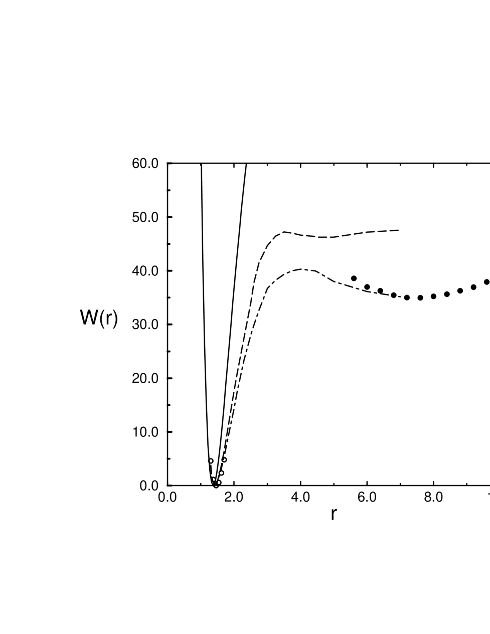
FIG. 1.: Potential of mean force in units of kcal/mol for bulk phase systems: solid line, bare potential; dashed lines, ACN; dashed-dotted lines, DMSO; open circles correspond to unconstrained trajectories results for DMSO and ACN at small distances; filled circles correspond to unconstrained trajectories results for DMSO at large distances. The distance $r$ is in units of Å.

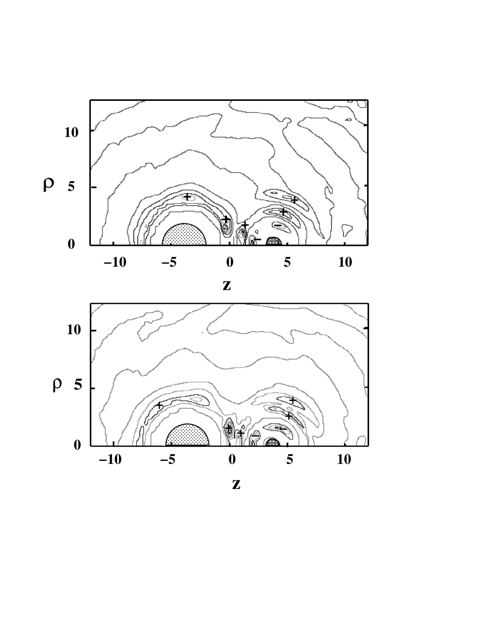
FIG. 2.: Contour plots of the charge density $n_{q}$ in the $\rho z$-plane with the ion pair in the SSIP configuration at $r=7.5$ Å. Top and bottom panels correspond to DMSO and ACN, respectively.

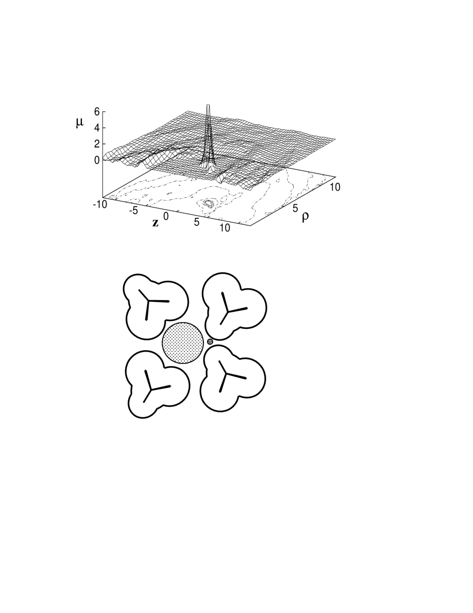
FIG. 3.: Dipolar density $n_{\mu}$ (written as $\mu$ on the ordinate) with the ion pair at $r=2.64$ Å: (a) ACN and (b) DMSO. Schematic representations of the local solvent structure are shown in the botton parts of the figures.

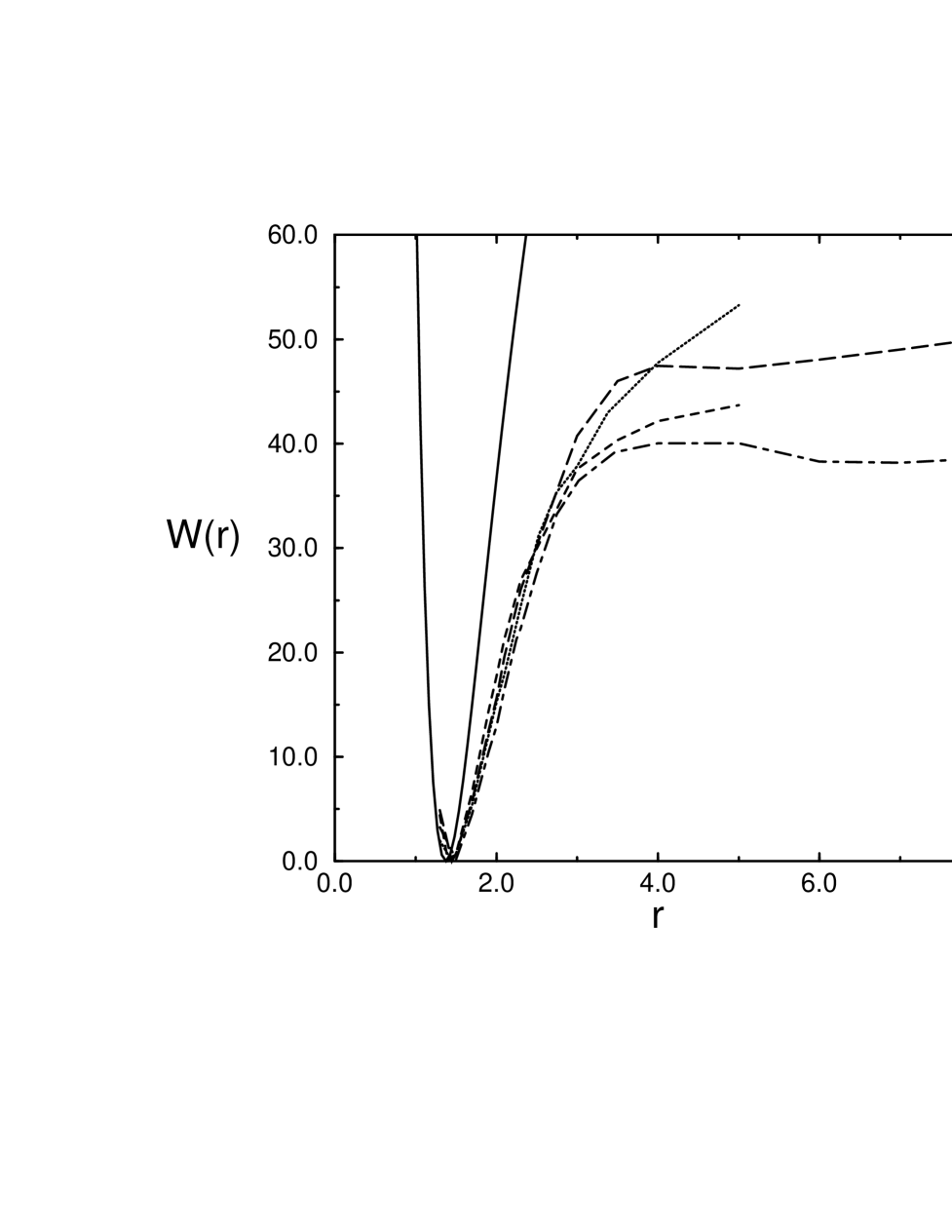
FIG. 4.: Potential of mean force for clusters: solid line, bare potential; dashed line, ACN cluster $n=14$; dotted line, ACN cluster $n=4$; dotted-dashed line, DMSO cluster $n=30$; short-dashed lines, ACN cluster $n=14$ treating the proton classically. Units are the same as in Fig. 1.

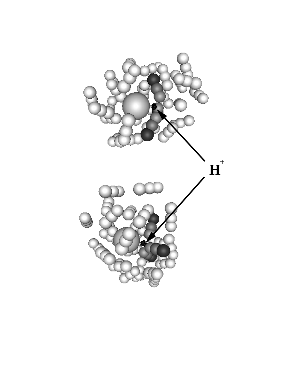
FIG. 5.: Two configurations of an $n=30$ ACN cluster with $r=2.64$ Å. The molecules strongly solvating H⁺ are heavily shaded and the two configuration illustrate the different orientations of the solvent molecules around H⁺.

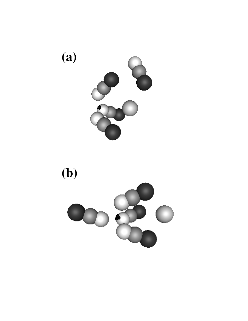
FIG. 6.: ACN cluster with $n=4$ with the ion pair fixed at $r=5.29$ Å. Parts (a) and (b) show two different metastable configurations.

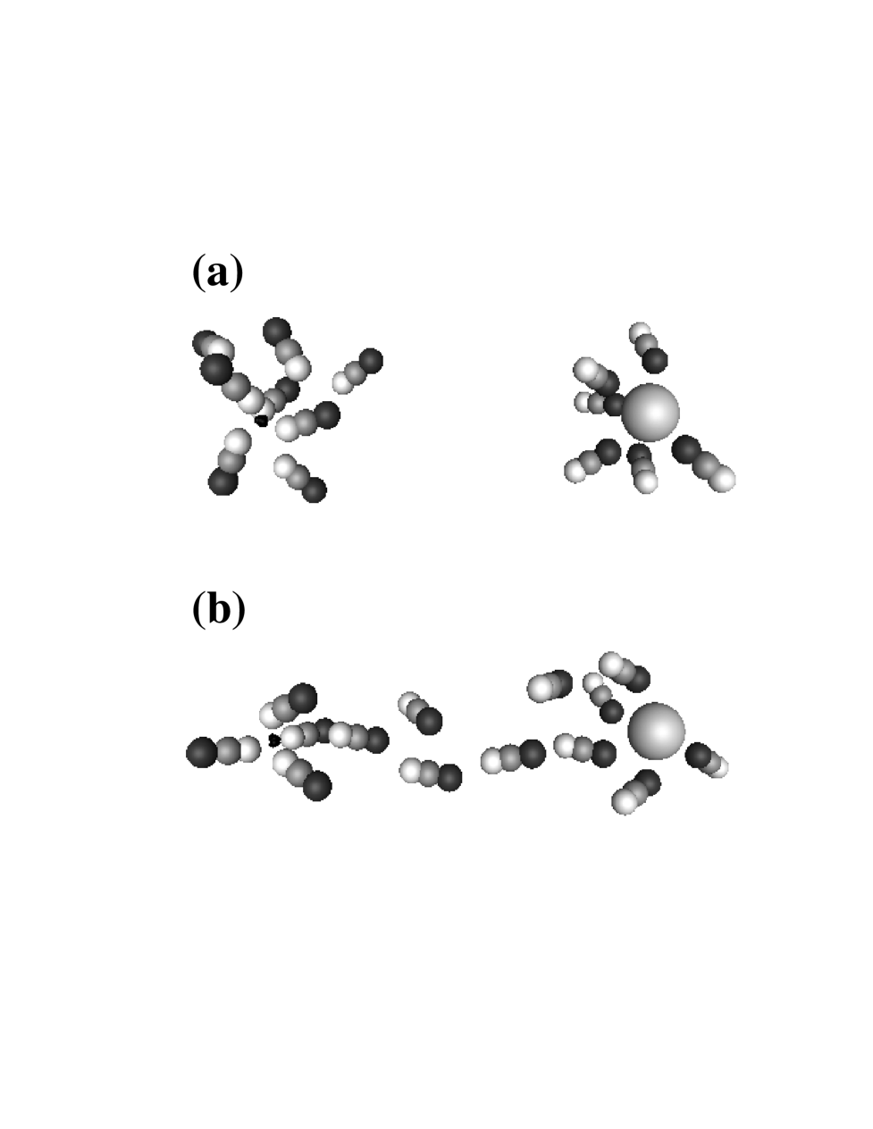
FIG. 7.: ACN cluster with $n=14$ and the ion pair distance fixed at $r=27$ Å. Parts (a) and (b) are two prominent metastable configurations.

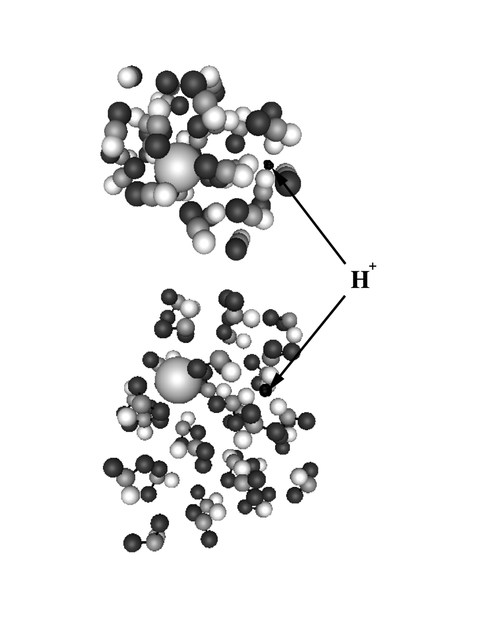
FIG. 8.: Two clusters with $n=30$ showing the solvent structure with the ion pair distance fixed at $r=7.5$ Å. Top, ACN; bottom, DMSO.

REFERENCES

- [1] C. Cooke, C. McCallum, A.D. Pethybridge and J.E. Prue, Electrochim. Acta, 20, 591 (1975). I.M. Kolthodd, S. Bruchenstein and M.K. Chantooni, Jr. J. Am. Chem. Soc. 83, 3927 (1961).
- [2] For a discussion of this mechanism see, for example, S. Glasstone, Physical Chemistry, (D. Van Nostrand Company, New York, 1959).
- [3] For a recent theoretical study of such effects for HCl ionization in water see, K. Ando and J.T. Hynes, J. Am. Chem. Soc., to be published.
- [4] S. Winstein, E. Clippenger, A.H. Fainber and G.C. Robinson, J. Am. Chem. Soc. 76, 259 (1954).
- [5] Simulations of SSIP configurations for classical ions in various model solvents have been carried out. See, for instance, O.A. Karim and J.A. McCammon, J. Am. Chem. Soc. 108, 1762 (1986); Chem. Phys. Lett. 132, 219 (1986); G. Ciccotti, M. Ferrario, J.T. Hynes and R. Kapral, Chem. Phys. 129, 241 (1989); J. Chem. Phys. 93, 7137 (1990).
- [6] O. Cheshnovsky and S. Leutwyler, Chem. Phys. Lett. 121, 1 (1985); R. Knochenmuss, O. Cheshnovsky and S. Leutwyler, , 144, 317 (1988).
- [7] J. A. Syage and J. Steadman, J. Chem. Phys. 95, 2497 (1991).
- [8] B. D. Kay, V. Hermann and A. W. Castleman, Jr., Chem. Phys. Lett. 80, 469 (1981).
- [9] J.P. Ryckaert, G. Ciccotti and H. J. C. Berendsen, J. Comput. Phys., 23, 327 (1977).
- [10] D.M.F. Edwards, P.A. Madden and I.R. McDonald, Mol. Phys. 51, 1141 (1984).
- [11] W. Feder, H. Dreizler, H.D. Rudolph and V. Typke, Z. Naturforsch. 24A, 266 (1969).
- [12] B.G. Rao and U.C. Singh, J. Am. Chem. Soc. 112, 3802 (1990).
- [13] S.H. Vosko, L. Wilk and M. Nusair. Can. J. Phys. 58, 1200 (1980). A.D. Becke. Phys. Rev. A 38, 3098 (1988). J.P. Perdew. Phys. Rev. B 33, 8800 (1986).
- [14] E. Clementi, S.J. Chakravorty, G.Corongiu, J.R. Flores and V. Sonnad. , Chapt. 2. edited by E. Clementi. (ESCOM, Leiden, 1991).
- [15] B.M. Pettitt and P. Rossky, J. Chem. Phys. 84, 5836 (1986).
- [16] R. P. Feynman, Statistical Mechanics (Addison Wesley, Reading, 1972).
- [17] D. Chandler and P. Wolynes, J. Chem. Phys. 74, 4078 (1981).
- [18] S. Nosé, Mol. Phys. 57, 187 (1986)
- [19] L. Verlet, Phys. Rev. 159, 98 (1967).
- [20] The calculation is similar to that for proton transfer: D.Laria, G.Ciccotti, M.Ferrario and R.Kapral, Chem. Phys. 180, 181 (1994).
- [21] M. Gillan, J. Phys. C 20, 3621 (1987).
- [22] G. A. Voth, D. Chandler and W. H. Miller, J. Chem. Phys. 91, 7749 (1989).
- [23] E. A. Carter, G. Ciccotti, J. T. Hynes and R. Kapral, Chem. Phys. Lett. 156, 472 (1989).
- [24] D. Laria and R. Fernández-Prini, J. Chem. Phys., 102, (1995).