The Nosé–Hoover thermostated Lorentz gas

Abstract

We apply the Nosé–Hoover thermostat and three variations of it, which control different combinations of velocity moments, to the periodic Lorentz gas. Switching on an external electric field leads to nonequilibrium steady states for the four models with a constant average kinetic energy of the moving particle. We study the probability density, the conductivity and the attractor in nonequilibrium and compare the results to the Gaussian thermostated Lorentz gas and to the Lorentz gas as thermostated by deterministic scattering.

I introduction

In a system of particles under an external force a nonequilibrium steady state can be obtained by applying a thermostat [1, 2, 3]. Deterministic and time reversible bulk thermostating is based on introducing a momentum dependent friction coefficient in the equations of motion. One type of this mechanism is the Nosé–Hoover thermostat [4, 5]. It creates a canonical ensemble in equilibrium and yields a stationary nonequilibrium distribution of velocities in nonequilibrium. Another version, the Gaussian isokinetic thermostat [6, 7, 8], leads to a microcanonical density for the velocity components in equilibrium and to a constant kinetic energy in nonequilibrium. Though the microscopic dynamics of these thermostated systems is time reversible the macroscopic dynamics is irreversible in nonequilibrium [9]. This is related to a contraction onto a fractal attractor [10, 11, 12].

Characteristic features of thermostated many particle systems, like a nonequilibrium steady state and a fractal attractor, have been recovered for a specific one particle system, the Gaussian thermostated Lorentz gas [10, 13, 14, 15, 16]. The periodic Lorentz gas consists of a particle that moves through a triangular lattice of hard disks and is elastically reflected at a collision with a disk. It serves as a standard model in the field of chaos and transport, see e. g., [3, 10]. In contrast to many particle systems a one particle system reflects more strongly the properties of a thermostat. For the Gaussian thermostated Lorentz gas a complicated dependence of the attractor on the field strength results [10, 13, 14].

A second simple one particle system which has been much investigated concerning its chaotic properties is the Nosé–Hoover thermostated harmonic oscillator. In contrast to the Lorentz gas, the dynamics of this system is generically nonergodic [18, 19]. However, one can obtain an ergodic dynamics for this system by the additional control of the square of the kinetic energy [19, 20, 21].

Recently an alternative thermostating mechanism, called thermostating by deterministic scattering, has been introduced for the periodic Lorentz gas [22, 23]. This deterministic and time reversible mechanism is based on including energy transfer between moving particle and disk scatterer at a collision, instead of using a momentum dependent friction coefficient. It leads to a canonical probability density for the particle in equilibrium, and in nonequilibrium it keeps the energy of the particle on average constant. In Refs. [22, 23] this model has been compared to the Gaussian thermostated Lorentz gas: In nonequilibrium one finds an attractor for this model which is similar to the fractal attractor of the Gaussian thermostated Lorentz gas, but in contrast to the Gaussian case the attractor is phase space filling even for high field strengths. For both models the conductivity is a nonlinear decreasing function with increasing field strength on a coarse scale.

Based on its construction the method of thermostating by deterministic scattering is in fact closer to the Nosé–Hoover thermostat. This motivates us to apply for the first time the Nosé–Hoover thermostat to the periodic Lorentz gas. In Section II we introduce the Nosé–Hoover thermostat and discuss some variations of it. In Section III we define the periodic Lorentz gas and the thermostats we will study. We investigate these models in equilibrium in section IV and in nonequilibrium in Section V. Conclusions are drawn in Section VI.

II The Nosé–Hoover thermostat and some variations

In the following sections we consider a one particle system in two dimensions with the position coordinates $\vec{q}=(q_{x},q_{y})$ and the momentum coordinates $\vec{p}=(p_{x},p_{y})$. The mass of the particle has been set equal to unity. The equations of motion for the Nosé–Hoover thermostat are then given by [5]

$$\dot{\vec{q}} = \vec{p}$$ (1)

$$\dot{\vec{p}} = \vec{\varepsilon}-\zeta\vec{p}$$ (2)

$$\dot{\zeta} = (\frac{p^{2}}{2T}-1)\frac{1}{\tau^{2}}\;.$$ (3)

The thermostat variable $\zeta$ couples the particle dynamics to a reservoir. It controls the kinetic energy of the particle $p^{2}/2$ such that $<p^{2}>=2T$. This holds even in nonequilibrium as induced by an electric field $\vec{\varepsilon}$. $\tau$ is the response time of the thermostat. Performing the limit $\tau\to 0$ in Eqs. (3) approximates the Gaussian thermostat with $\zeta=(\vec{\varepsilon}\cdot\vec{p})/p^{2}$. In the limit $\tau\to\infty$ the friction coefficient approaches a constant, $\zeta=\zeta_{c}$, and the equations of motion are not time reversible anymore. The dynamics of this dissipative limit has been investigated in [25].

A generalization of the Nosé–Hoover thermostat to control higher even moments of $p$ has been introduced by Hoover [26]. The moments are fixed according to the momentum relations for the Gaussian distribution. By such a more detailed control of the nonequilibrium steady state statistical dynamical properties, like ergodicity, can be improved, as has been mentioned for the Nosé–Hoover thermostated harmonic oscillator in the introduction. In principle the method of the control of the even moments can straightforwardly be extended to the control of the odd moments. However, such a thermostat would involve an additional parameter to control the respective current of the subsystem. Thus, the corresponding reservoir would be more than a single thermal reservoir, which is physically not desirable, apart from the fact that the respective equations of motion would not be time reversible anymore.

We briefly note that there exist other formal generalizations [27], or modifications [28, 29], of the Nosé–Hoover thermostat in the literature. They have been critically reviewed in Refs. [20, 21, 26].

III Variations of the Nosé–Hoover thermostat for the periodic Lorentz gas

The basic themostating method we investigate in this paper is the Nosé–Hoover thermostat, Eqs. (3). In the following we introduce three variations of it which are time reversible and result in a dissipative dynamics in nonequilibrium.

The first variation is the Nosé–Hoover thermostat with a field dependent coupling to the reservoir,

$$\dot{\vec{q}} = \vec{p}$$ (4)

$$\dot{p_{x}} = \varepsilon_{x}-(1+\varepsilon_{x})\zeta p_{x}$$ (5)

$$\dot{p_{y}} = \varepsilon_{y}-(1+\varepsilon_{y})\zeta p_{y}$$ (6)

$$\dot{\zeta} = (\frac{p^{2}}{2T}-1)\frac{1}{\tau^{2}}\;,$$ (7)

which is obtained by including the factors $1+\varepsilon_{x}$, resp. $1+\varepsilon_{y}$, in Eqs. (3). Alternatively, these equations can be written by defining two field dependent friction coefficients, $\xi_{x}=(1+\varepsilon_{x})\zeta$ and $\xi_{y}=(1+\varepsilon_{y})\zeta$, which are governed by $\dot{\xi}_{x}=(p^{2}/2T-1)(1+\varepsilon_{x})/\tau^{2}$ and $\dot{\xi}_{y}=(p^{2}/2T-1)(1+\varepsilon_{y})/\tau^{2}$, respectively. It then becomes clear that for each momentum component there exists a separate response time of the reservoir which reads $\tau/\sqrt{1+\varepsilon_{x}}$, resp. $\tau/\sqrt{1+\varepsilon_{y}}$. The basic advantage of this thermostat is that the response times are now adjusted to the corresponding component of the field strength such that with increasing field strength the response time decreases. The standard Nosé–Hoover thermostat Eqs. (3) is contained as a special case in equilibrium .

The second variation goes back to Hoover [26]. It includes a control of $<p^{4}>=8T^{2}$,

$$\dot{\vec{q}} = \vec{p}$$ (8)

$$\dot{\vec{p}} = \vec{\varepsilon}-\zeta_{1}\vec{p}-\zeta_{2}\frac{p^{2}}{2T}\vec{p}$$ (9)

$$\dot{\zeta_{1}} = (\frac{p^{2}}{2T}-1)\frac{1}{\tau^{2}}$$ (10)

$$\dot{\zeta_{2}} = \frac{p^{2}}{2T}(\frac{p^{2}}{2T}-2)\frac{1}{\tau^{2}}\;.$$ (11)

As mentioned in the previous sections this variation can improve statistical dynamical properties, like ergodicity.

The third variation controls $p_{x}^{2}$ and $p_{y}^{2}$ separately. This is performed by defining two independent reservoirs for the $x$– and $y$–direction,

$$\dot{\vec{q}} = \vec{p}$$ (12)

$$\dot{p_{x}} = \varepsilon_{x}-\zeta_{x}p_{x}$$ (13)

$$\dot{p_{y}} = \varepsilon_{y}-\zeta_{y}p_{y}$$ (14)

$$\dot{\zeta_{x}} = (\frac{p_{x}^{2}}{T}-1)\frac{1}{\tau^{2}_{x}}$$ (15)

$$\dot{\zeta_{y}} = (\frac{p_{y}^{2}}{T}-1)\frac{1}{\tau^{2}_{y}}\;.$$ (16)

This variation more deeply intervenes in the microscopic dynamics by forcing the single components $p_{x}^{2}$ and $p_{y}^{2}$ separately towards canonical distributions. However, in contrast to the previous variations a curiosity is hidden in it: At a collision the thermostat $\zeta_{x},\zeta_{y}$ is uncorrelated to the thermostated variables $p_{x}$ and $p_{y}$, because $p_{x}$ and $p_{y}$ change at a collision whereas $\zeta_{x},\zeta_{y}$ remain the same. Therefore the thermostat does not work efficiently. But we have not found any reflection of this curiosity in the macroscopic behavior.

We study the dynamics of these models in one Lorentz gas cell with periodic boundaries, see Fig. 1(a). As the radius of the disk we take $r=1$. For the spacing between two neighboring disks we choose $w\simeq 0.2361$, corresponding to a density equal to $4/5$ of the maximum packing density of the scatterers. A collisionless free flight of the particle is avoided for this parameter [10]. The relevant variables of the dynamical system are defined in Fig. 1(b): $\beta$ is the angular coordinate of the point at which the particle elastically collides with the disk, and $\gamma$ is the angle of incidence at this point.

The equations of motion are integrated by a fourth order Runge Kutta algorithm with a step size of $dt=0.005$ between two collisions. The collision of the particle with the disk has been determined with a precision of $10^{-7}$. Unless declared otherwise the temperature is chosen to $T=0.5$.

IV Equilibrium

Inserting the initial condition $(p_{0},\zeta_{0})=(\sqrt{2T},0)$ in Eqs. (3) with $\varepsilon=0$ the velocity of the particle becomes a constant, $p=\sqrt{2T}$, that means the Nosé–Hoover thermostat does not act in the Lorentz gas and the dynamics is microcanonical. For other initial conditions one observes in computer simulations that $p^{2}$ and $\zeta$ oscillate periodically and that the dynamics of this one particle system is nonergodic.

A stability analysis confirms the numerical results: The Nosé–Hoover thermostated equations of motion Eqs. (3) can be reduced for $\varepsilon=0$ to

$$\dot{p^{2}} = -2\zeta p^{2}$$ (17)

$$\dot{\zeta} = (\frac{p^{2}}{2T}-1)\frac{1}{\tau^{2}}\;.$$ (18)

Eqs. (18) are also valid at the moment of a collision, because $p^{2}$ and $\zeta$ are not changed by a collision. The fixed point of Eqs. (18) is $(p^{2},\zeta)=(2T,0)$ with the eigenvalues $\lambda_{1/2}=\pm\sqrt{-4T/\tau^{2}}$ and is thus elliptic.

The additional control of $<p^{4}>$ destroys the microcanonical probability density but it is not sufficient to obtain an “exact” dynamics in the periodic Lorentz gas. Different initial conditions still lead to a different shape of the probability density $\varrho(p_{x})$, as is shown in Fig. 2(a).

In contrast the separate control of $p_{x}^{2}$ and $p_{y}^{2}$ leads to an exact dynamics in equilibrium corresponding to the canonical probability density $\varrho(p_{x})$, as shown in Fig. 2(b).

V Nonequilibrium

We now apply an external electric field $\vec{\varepsilon}$ parallel to the $x$–axis. The Nosé–Hoover thermostat and the related models then lead to well defined nonequilibrium steady states with constant average energy of the particle.

A Probability density $\varrho(p_{x})$

The probability density $\varrho(p_{x})$ for the Nosé–Hoover thermostat for $\varepsilon=0.5$ is presented in Fig. 3(a). For $\tau^{2}=0.01$ the density shows some remains of the deformed microcanonical density of the Gaussian thermostat, whereas for $\tau^{2}=1$ and $\tau^{2}=1000$ the density becomes similar to the density of thermostating by deterministic scattering, which is related to a canonical distribution [22, 23].

Fig. 3(b) shows $\varrho(p_{x})$ for the three variations of the Nosé–Hoover thermostat. We have chosen here $T=0.60029$ which corresponds to the temperature in the bulk for thermostating by deterministic scattering at a parametric temperature of $T=0.5$. The density of the Nosé–Hoover thermostat with field dependent coupling to the reservoir is very close to the density of thermostating by deterministic scattering. The density of the Nosé–Hoover thermostat with separate control of $p_{x}^{2}$ and $p_{y}^{2}$ looks like a superposition of the densities of the Nosé–Hoover thermostat for small and for large $\tau$.

In all models the mean value of $\varrho(p_{x})$ is positive, indicating a current parallel to the field direction.

B Conductivity

The conductivity $\sigma=<p_{x}>/\varepsilon$ for the Nosé–Hoover thermostat is shown in Fig. 4. For $\tau^{2}=0.01$ the curve is very similar to the conductivity of the Gaussian thermostated Lorentz gas [14]. For $\tau^{2}=1000$ the curve is more stretched along the $\varepsilon$–axis and globally not decreasing anymore. In contrast the conductivity as obtained from thermostating by deterministic scattering [22, 23] is a globally decreasing function. According to the Einstein relation, in the limit $\varepsilon\to 0$ $\sigma$ should approach the equilibrium diffusion coefficient $D$ of the periodic Lorentz gas, which for $w=0.2361$ has the value $D\approx 0.21$ [15]. This is hard to see for $\tau^{2}=1000$, because for $\varepsilon\to 0$ the probability density changes drastically from a smooth, canonical like density to a non-smooth density. It is also difficult to see any linear response in computer simulations, as has already been discussed for the Gaussian thermostated Lorentz gas and for thermostating by deterministic scattering in Ref. [23].

C Attractor

Fig. 5 shows the Poincaré section of $(\beta,\sin(\gamma))$ at the moment of the collision for the Nosé–Hoover thermostat, for the three variations and for thermostating by deterministic scattering. Again, we have chosen $T=0.60029$ to compare the results with thermostating by deterministic scattering. For all models the structure of the attractor is qualitatively the same as the structure of the fractal attractor obtained for the Gaussian thermostated Lorentz gas [10]. However, the fine structure varies with the models and with the response time $\tau$. For the Nosé–Hoover thermostat with $\tau^{2}=0.01$, see Fig 5(a), the structure is most pronounced, whereas for the control of $p_{x}^{2}$ and $p_{y}^{2}$ separately, see Fig. 5(e), the structure is least visible.

D Bifurcation diagram

The angle $\beta$ at the moment of the collision is presented as a function of the field strength for the Nosé–Hoover thermostat in Fig. 6. For all three values of $\tau^{2}$ the attractor is phase space filling for small field strengths $\varepsilon<1.3$ and contracts onto a periodic orbit with increasing field strength. For $\tau^{2}=0.01$ the scenario is similar to the one of the Gaussian thermostated Lorentz gas [14]. For $\tau^{2}=1$ the scenario looses its richness, but it gets a bit more complicated again for $\tau^{2}=1000$. In contrast to the Nosé–Hoover thermostat, the attractor of thermostating by deterministic scattering remains phase space filling even for large $\varepsilon$ [22, 23].

The bifurcation diagram in the dissipative limit $\tau\to\infty$ of Eqs. (3) with a constant friction coefficient $\zeta_{c}$ shows an inverse scenario to Fig. 6, as is presented in Fig. 7. For small $\varepsilon$ the trajectory is a so–called creeping orbit [25], then it changes to a periodic orbit, and for large $\varepsilon$ the attractor gets phase space filling. By increasing $\zeta_{c}$ the strength of the dissipation increases with the consequence that the onset of chaotic behavior starts at higher field strengths. With respect to the numerics we remark that related to the different shapes of the attractors by varying $\zeta_{c}$ in the dissipative limit, the duration of the transient behavior of the Nosé–Hoover thermostat grows drastically for $\tau\to\infty$.

Figs. 8-10 show the bifurcation diagrams for the three variations of the Nosé–Hoover thermostat. In general one observes that even for high field strengths chaotic regions appear, in contrast to the Nosé–Hoover thermostat.

For the variation with the additional control of $p^{4}$ the attractor covers a bounded $\beta$–interval for $\varepsilon\geq 3$. For these field strengths the trajectory is a creeping orbit.

Fig. 10(b) depicts the attractor for the variation with separate control of $p_{x}^{2}$ and $p_{y}^{2}$ under different response times for the $x$– and $y$–direction. Since the field acts in the $x$–direction we have chosen a strong coupling, $\tau^{2}_{x}=0.1$, for the $x$–direction and a weak coupling, $\tau^{2}_{y}=1000$, for the y–direction. Up to a field strength $\varepsilon\approx 6.5$ no periodic window has been found. The bifurcation diagram for these parameters most strongly deviates from the Nosé–Hoover and Gaussian thermostated Lorentz gas and is closest to the bifurcation diagram of thermostating by deterministic scattering. However, in contrast to thermostating by deterministic scattering the attractor is more concentrated around $\beta\simeq\pi$.

We detected a numerical problem for the second and the third variation at several values of $\tau$. One observes that sporadically after large time intervals there appears a creeping orbit with a very low velocity of the particle, which is difficult to handle numerically. Whether this creeping orbit is the stationary state could probably be clarified by calculating Lyapunov exponents [15].

E Thermodynamic entropy production and phase space volume contraction

A characteristic property of the Nosé–Hoover thermostat as well as of the Gaussian isokinetic thermostat is that the thermodynamic entropy production is equal to the phase space volume contraction rate [9]. This equality can as well easily be verified for the variation with the additional control of $p^{4}$ and for the variation with separate control of $p_{x}^{2}$ and $p_{y}^{2}$.

On the other hand it does not hold for the Nosé–Hoover thermostat with field dependent coupling to the reservoir. From Eqs. (7) one gets for the phase space contraction rate of this model $-<\rm{div}\dot{\Gamma}>=(2+\varepsilon)<\zeta>$ where $\dot{\Gamma}=(\dot{\vec{q}},\dot{\vec{p}},\dot{\zeta})$. The precise relation between thermodynamic entropy production $\dot{S}_{TD}=\varepsilon<p_{x}>/T$ and $-<\rm{div}\dot{\Gamma}>$ for this variation is obtained by calculating the energy balance between subsystem and reservoir:

$$E=\frac{p^{2}}{2}+T\tau^{2}\zeta^{2}$$ (19)

is the total energy which in a nonequilibrium steady state should on average be zero,

$$<\frac{dE}{dt}>=0\;.$$ (20)

Inserting Eqs. (7) with $\varepsilon_{y}=0$ in Eqs. (20) leads to

$$\frac{\varepsilon_{x}<p_{x}>}{T}=\frac{\varepsilon_{x}<p_{x}^{2}\zeta>}{T}+2<\zeta>\;.$$ (21)

Numerical simulations have shown that $p_{x}^{2}$ and $\zeta$ are no independent quantities in nonequilibrium. If $p_{x}^{2}$ and $\zeta$ would be independent and equipartitioning would be fulfilled, i. e., $<p_{x}^{2}>=T$, which is only the case in equilibrium, then Eq. (21) would lead to an identity between thermodynamic entropy production and phase space volume contraction. The results for $-<\rm{div}\dot{\Gamma}>$ and for $\dot{S}_{TD}$ as obtained from computer simulations for this system are presented in Table I at different $\tau$ and $\varepsilon$. More details of the entropy production in this variation and in a Gaussian thermostat with the same property are discussed in Ref. [31].

VI conclusions

We have investigated the Nosé–Hoover thermostat and three variations of it for the periodic Lorentz gas. All models are time reversible and lead to well defined nonequilibrium steady states with a constant average kinetic energy of the moving particle.

As a typical characteristic of deterministic and time reversible thermostating mechanisms it has been confirmed that in nonequilibrium all these systems contract onto attractors similar to the fractal attractor of the Gaussian thermostated Lorentz gas.

In equilibrium only the variation of the Nosé–Hoover thermostat with separate control of $p_{x}^{2}$ and $p_{y}^{2}$ leads to an exact dynamics with $\varrho(p_{x})$ being canonical just like the corresponding density of thermostating by deterministic scatterin g.

In nonequilibrium the attractor of the Nosé–Hoover thermostat contracts onto a periodic orbit for higher field strength, analogous to the Gaussian thermostated Lorentz gas. However, the detailed scenario depends on the value of the response time $\tau$. Concerning the probability density in equilibrium, the attractor, and the conductivity in nonequilibrium, the properties of the standard Nosé–Hoover thermostat in the periodic Lorentz gas are closer to the properties of the Gaussian thermostat than to the properties of thermostating by deterministic scattering, although the Nosé–Hoover thermostat and thermostating by deterministic scattering share the property of keeping the energy of the particle on average constant in nonequilibrium, and for both thermostats the probability densities for the velocity components are related to a canonical probability density.

Concerning the bifurcation diagrams we find that the dynamics of the three variations of the Nosé–Hoover thermostat are in general “more chaotic”. Even for higher field strengths there exist pronounced chaotic regions. The separate control of $p_{x}^{2}$ and $p_{y}^{2}$ leads to a phase space filling attractor up to high field strengths in nonequilibrium. The equilibrium properties and the bifurcation diagram in nonequilibrium of this model are qualitatively closest to the properties of thermostating by deterministic scattering in comparison to the other versions.

For the Nosé–Hoover thermostat with field dependent coupling to the reservoir the thermodynamic entropy production is generically not equal to the phase space volume contraction in contrast to the other models.

An important question would be to look for common properties of all deterministic and time reversible thermostats. So far, only the existence of a fractal attractor in nonequilibrium appears to be typical. A more detailed investigation of these thermostating mechanisms should in particular involve a quantitative comparison, as, e. g., by means of computing Lyapunov exponents. An answer to this question would be helpful for obtaining a general characterization of nonequilibrium steady states.

Acknowledgments: We dedicate this article to G. Nicolis, a champion of chaoticity, on occasion of his 60th birthday. K. R. and R. K. thank G. Nicolis for his continuous support and for the possibility to collaborate with him on problems of thermostating. This work has been started during the workshop “Nonequilibrium Statistical Mechanics” (Vienna, February 1999). The authors thank the organizers G. Gallavotti, H. Spohn and H. Posch for the invitation to this meeting. K. R. thanks the European Commission for a TMR grant under contract no. ERBFMBICT96-1193. R. K. acknowledges as well financial support from the European Commission.

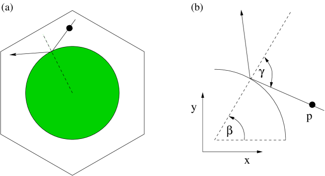
FIG. 1.: (a) Elementary cell of the periodic Lorentz gas on a triangular lattice. (b) Definition of the relevant variables.

FIG. 2.: Probability density $\varrho(p_{x})$ for $\varepsilon=0$: (a) additional control of $<p^{4}>$ with $\tau^{2}=1$ at two different initial conditions, (b) control of $<p_{x}^{2}>$ and $<p_{y}^{2}>$ separately with $\tau^{2}_{x}=0.1$ and $\tau^{2}_{y}=1000$

FIG. 3.: Probability density $\varrho(p_{x})$ for $\varepsilon=0.5$: (a) Nosé–Hoover thermostat with $\tau^{2}=0.01$ (dotted curve), $\tau^{2}=1$ (dashed curve), $\tau^{2}=1000$ (long dashed curve) and thermostating by deterministic scattering (solid curve), (b) Nosé–Hoover thermostat with field dependent coupling to the reservoir with $\tau^{2}=1$ (dotted curve), additional control of $<p^{4}>$ with $\tau^{2}=1$ (dashed curve), control of $<p_{x}^{2}>$ and $<p_{y}^{2}>$ separately with $\tau^{2}_{x}=0.1$ and $\tau^{2}_{y}=1000$ (long dashed curve) and thermostating by deterministic scattering (solid curve).

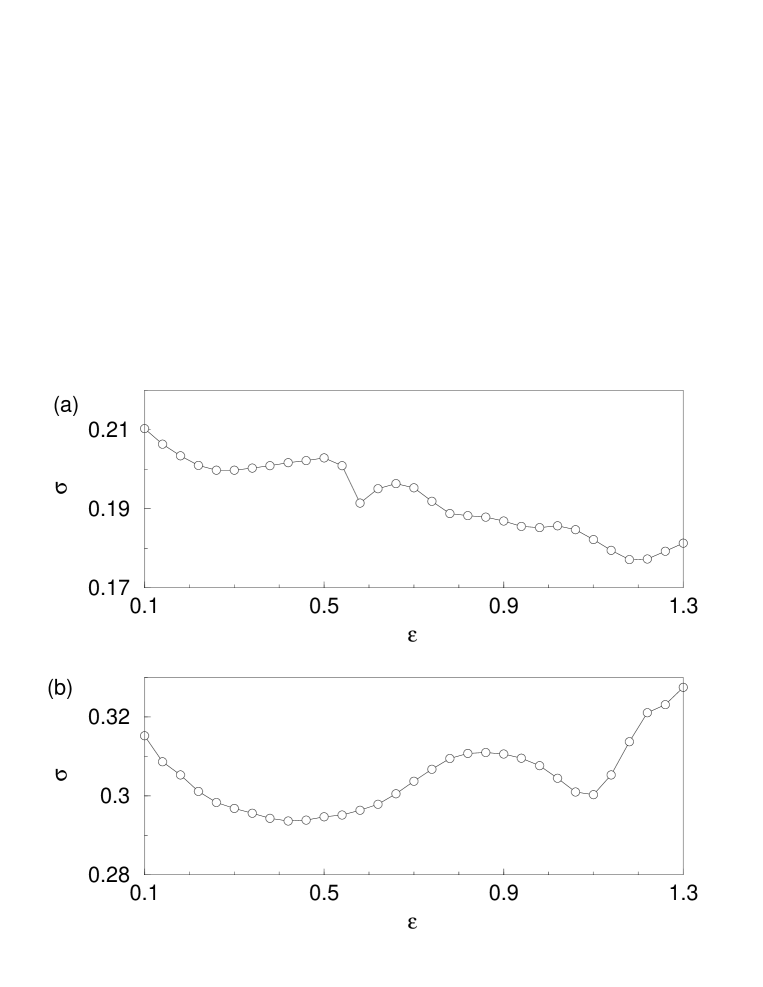
FIG. 4.: Conductivity $\sigma$ for the Nosé–Hoover thermostat, (a) $\tau^{2}=0.01$, (b) $\tau^{2}=1000$. The numerical uncertainty of each point is less then symbol size.

FIG. 5.: Poincaré section of $(\beta,\sin\gamma)$, as defined in Fig. 1 at the moment of the collision, for field strength $\varepsilon=1$: Nosé–Hoover thermostat (a) $\tau^{2}=0.01$, (b) $\tau^{2}=1000$, (c) Nosé–Hoover thermostat with field dependent coupling to the reservoir, $\tau^{2}=1$ (d) additional control of $p^{4}$, $\tau^{2}=1$, (e) control of $p_{x}^{2}$ and $p_{y}^{2}$ separately, $\tau^{2}_{x}=0.1$ and $\tau^{2}_{y}=1000$, and (f) thermostating by deterministic scattering.

FIG. 6.: bifurcation diagram for the Nosé–Hoover thermostat (a) $\tau^{2}=0.01$, (b) $\tau^{2}=1$, (c) $\tau^{2}=1000$

FIG. 7.: bifurcation diagram for the dissipative limit (a) $\zeta_{c}=1.0$, (b) $\zeta_{c}=2.0$

FIG. 8.: bifurcation diagram for the variation with field dependent coupling to the reservoir, $\tau^{2}=1$

FIG. 9.: bifurcation diagram for the additional control of $p^{4}$, $\tau^{2}=1$

FIG. 10.: bifurcation diagram for the control of $p_{x}^{2}$ and $p_{y}^{2}$ separately, (a) $\tau^{2}_{x}=\tau^{2}_{y}=1$, (b) $\tau^{2}_{x}=0.1$, $\tau^{2}_{y}=1000$

TABLE I.: Phase space volume contraction rate and thermodynamic entropy production for the Nosé–Hoover thermostat with field dependent coupling to the reservoir. The numerical error is $\leq 0.001$

$\varepsilon$	$\tau^{2}=1$		$\tau^{2}=1000$
	$-<\rm{div}\dot{\Gamma}>$	$\dot{S}_{TD}$	$-<\rm{div}\dot{\Gamma}>$	$\dot{S}_{TD}$
0.5	0.152	0.145	0.145	0.147
1.0	0.547	0.561	0.567	0.592
1.5	1.240	1.366	1.256	1.391

REFERENCES

- [1] D. J. Evans and G. P. Morriss, Statistical Mechanics of Nonequilibrium Liquids (Academic Press, London, 1990).
- [2] W. G. Hoover, Computational statistical mechanics (Elsevier, Amsterdam, 1991).
- [3] G. P. Morriss and C. P. Dettmann, Chaos 8, 321 (1998).
- [4] S. Nosé, J. Chem. Phys. 81, 511 (1984).
- [5] W. G. Hoover, Phys. Rev. A 31, 1695 (1985).
- [6] W. G. Hoover, A. J. C. Ladd, and B. Moran, Phys. Rev. Lett. 48, 1818 (1982).
- [7] D. J. Evans, J. Chem. Phys. 78, 3297 (1983).
- [8] D. J. Evans et al., Phys. Rev. A 28, 1016 (1983).
- [9] B. L. Holian, W. G. Hoover, and H. A. Posch, Phys. Rev. Lett. 59, 10 (1987).
- [10] B. Moran and W. G. Hoover, J. Stat. Phys. 48, 709 (1987).
- [11] G. P. Morriss, Phys. Lett. A 134, 307 (1989).
- [12] W. G. Hoover, Time Reversibility, Computer Simulation, and Chaos (World Scientific, Singapore, 1999).
- [13] J. Lloyd, L. Rondoni, and G. P. Morriss, Phys. Rev. E 50, 3416 (1994).
- [14] J. Lloyd, M. Niemeyer, L. Rondoni, and G. P. Morriss, Chaos 5, 536 (1995).
- [15] C. Dellago, L. Glatz, and H. A. Posch, Phys. Rev. E 52, 4817 (1995).
- [16] C. P. Dettmann and G. P. Morriss, Phys. Rev. E 54, 4782 (1996).
- [17] M. Kac, Scientific American 211, 92 (1964).
- [18] H. A. Posch, W. G. Hoover, and F. J. Vesely, Phys. Rev. A 33, 4253 (1986).
- [19] H. A. Posch and W. G. Hoover, Phys Rev E 55, 6803 (1997).
- [20] W. G. Hoover and B. L. Holian, Phys. Lett. 211, 253 (1996).
- [21] W. G. Hoover and O. Kum, Phys Rev E 56, 5517 (1997).
- [22] R. Klages, K. Rateitschak, and G. Nicolis, preprint chao-dyn/9812021.
- [23] K. Rateitschak, R. Klages, and G. Nicolis, preprint chao-dyn/9908013.
- [24] C. Wagner, R. Klages, and G. Nicolis, Phys. Rev. E 60, 1401 (1999).
- [25] W. G. Hoover and B. Moran, Chaos 2, 599 (1992).
- [26] W. G. Hoover, Phys. Rev. 40, 2814 (1989).
- [27] J. Jellinek and R. S. Berry, Phys. Rev. A 38, 3069 (1988).
- [28] A. Bulgac and D. Kusnezov, Phys. Rev. A 42, 5045 (1990).
- [29] G. J. Martyna, M. L. Klein and M. Tuckerman, J. Chem. Phys. 97, 2635 (1992).
- [30] M. C. Mackey, Rev. Mod. Phys. 61, 981 (1989).
- [31] R. Klages and K. Rateitschak (unpublished).