[

Differential light scattering: probing the sonoluminescence collapse

Abstract

We have developed a light scattering technique based on differential measurement and polarization (differential light scattering, DLS) capable in principle of retrieving timing information with picosecond resolution without the need for fast electronics. DLS was applied to sonoluminescence, duplicating known results (sharp turnaround, self-similar collapse); the resolution was limited by intensity noise to about 0.5 ns. Preliminary evidence indicates a smooth turnaround on a $\lesssim 0.5$-ns time scale, and suggests the existence of subnanosecond features within a few nanoseconds of the turnaround.

]

Since Gaitan’s seminal work [2, 3], significant advances have been made in our understanding of single-bubble sonoluminescence (SL). The dissociation hypothesis (DH) introduced by Lohse et al. [4] combines the merits of an intuitive approach based on the relatively tractable Rayleigh-Plesset equation (RPE) of bubble dynamics with an impressive ability to reproduce a wide range of observables [5, 6, 7, 8, 9]. More sophisticated theories [10, 11] yield a more realistic picture of the phenomenon that is in general agreement with the results of the DH-RPE treatment. Experimentally, however, information on the bubble interior is still very scarce. In particular, no direct and conclusive evidence exists yet for either plasma formation or shock waves inside the collapsing bubble. As a result, many competing theories [12, 13, 14, 15, 16, 17, 18, 19] still vie with the adiabatic or shock-wave heating theory for the distinction of accurately describing the SL phenomenon. It seems desirable, then, to explore additional ways of probing the interior of the bubble with a time resolution comparable [20] to the duration of the flash, measured to be 40–380 ps [21, 22, 23, 24]. Light scattering has already been shown [25, 26, 27] to be a useful probe of the bubble dynamics, sensitive as it is to the dielectric interface at the bubble wall. It is also a promising candidate for detection of either plasma or shock waves, since both features can modulate substantially the local dielectric constant.

Our goal was to push measurements of the light scattering cross section of the collapsing bubble to a greater temporal resolution than that afforded by the pulsed Mie scattering technique [26], which appears to be limited to around $\frac{1}{2}$ ns by low light levels and the need for averaging. In order to achieve higher resolution, we have developed a technique called differential light scattering (DLS) that reduces statistical uncertainty in the detection process by making use of more powerful ultrafast laser pulses. Since DLS does not rely on a fiducial time reference, it, too, is completely insensitive to electronic timing noise, allowing the use of relatively slow detectors. The DLS technique is based on two central concepts: (i) using a differential measurement to yield jitter-free timing information, and (ii) using polarized light to generate such a measurement through scattering.

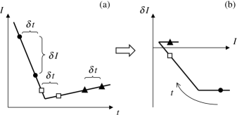
FIG. 1.: DLS concept applied to a simple curve. (a) Sampling of $I(t)$ occurs in pairs; (b) for each pair, the difference signal is plotted against the first signal. Equal symbols indicate the correspondence between (a) and (b). Notice the slanted “wall” in (b) resulting from the two samples lying on opposite sides of the sharp cusp in (a).

The differential measurement concept was recently introduced for the first time by Rella et al. in the context of ultrafast gating of optical pulses [28]. The technique they invented, differential optical gating (DOG), was used to measure the shape of a midinfrared pulse with subpicosecond resolution. Our technique applies the DOG concept to light scattering. DLS relies on collecting many pair of correlated samples of the same periodic event $I(t)$ (see Fig. 1). Each pair $i$ consists of the first sample $I(t_{i})$ and the second sample $I(t_{i}+\delta t)$, where $t_{i}$ is the time of the first sample (modulo the period $T$), and $\delta t$ is an appropriately chosen (and short) time delay. From each such pair, an intensity difference

$$\delta I_{i}=I(t_{i}+\delta t)-I(t_{i})$$ (1)

is produced and plotted against the first sample $I(t_{i})$, generating what we will call a DLS plot. When enough event pairs are collected, the points representing them in the DLS plot will join together in defining a continuous curve.

The DLS plot can be thought of as a predictor: given an intensity $I$ at some time $t$, the plot yields what $I$ will be after a time $\delta t$. One can numerically step along the curve on this plot to retrieve the desired direct function $I(t)$. Depending on the nature of the features of interest, in some cases it is more fruitful to plot, for each pair, $\delta I_{i}$ against the second sample $I(t_{i}+\delta t)$. The reconstruction of $I(t)$ is then carried out backwards in time. When the data are particularly noisy, however, features apparent in the DLS plot will be lost in the reconstruction process, eliminating any benefit of the technique. In this case, it is better to work directly in DLS space. Using a model for $I(t)$, a DLS curve can be generated from it by applying map (1), then fit to the data points in the DLS plot with a minimization algorithm.

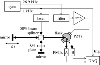
FIG. 2.: Experimental setup. Thin lines, electrical signals; thick lines, beam paths; dashed line, beam going into the page.

To implement the DLS concept (Fig. 2), a laser pulse is split equally in two and recombined as in a Michelson interferometer, with one pulse having traveled a longer path. The two-pulse train is focused onto the bubble, yielding two bursts of scattered light separated by an adjustable time delay $\delta t$. In order to distinguish between the two pulses during detection, an additional degree of freedom is needed. Color discrimination is a possibility, but with several drawbacks, among which the need for frequency doubling and the strong wavelength dependence of light scattering. Polarization, on the other hand, is perfectly suited to this technique. Calculations using Mie scattering theory [29], which is rigorously valid for spheres of arbitrary size, show that scattered intensities are highly polarization dependent. For the case of linearly polarized light, scattering at $\theta=90^{o}$ (where zero is forward) vanishes if the polarization vector e is parallel to the scattering plane. Therefore, the polarization of one of the pulses is made to rotate by $90^{o}$ (with the quarter-wave plate shown in Fig. 2) before the two pulses are recombined. Figure 3 shows the sequence of the two pulses scattering from the bubble. The first pulse scatters preferentially in the plane containing one photomultiplier tube (PMT), while the second pulse does so in the perpendicular plane, which contains the other PMT.

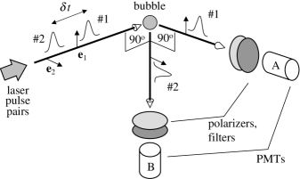
FIG. 3.: Scattering and polarization geometry. Not shown: lenses focus the input beam onto the bubble and relay scattered light onto the detectors.

Combining the time delay and the polarization dependence results in the ability to assign the scattered intensity recorded by one detector to the earlier pulse, and that recorded by the other detector to the later pulse. Therefore, each laser burst yields an ordered pair of scattered intensities. By scanning the arrival time of the pulse pairs over some portion of the acoustic cycle, enough data can be collected to generate a DLS plot of the desired interval of the bubble’s evolution.

The experiments were performed in a 100-ml spherical boiling flask filled with distilled, deionized water (resistivity $\rho=15.9$ M$\Omega$-cm) at $20\pm 1$ ^oC. The water was prepared in a gas-handling system under an air pressure of 0.2 bar, then loaded into the flask without further exposure to air. A sealed connection to a volume reservoir (kept at atmospheric pressure for these experiments) inspired by Ref. [30] provided pressure release from volume changes induced by temperature fluctuations. The entire assembly was leak tested; with the flask under vacuum, the rate of pressure rise was conservatively determined to be 16 nbar s^-1. However, under normal operating conditions the flask is filled with water and repressurized to 1 bar: this forces outside air to diffuse into the undersaturated water through microscopic interfaces, resulting in a substantially lower rate of contamination. The experiments described here took place 110 days after loading. Within that time, the pressure in an initially empty flask would have risen to roughly 0.2 bar; the air concentration in the water-filled flask can instead be expected to have risen by perhaps a few percent of atmospheric saturation.

The first acoustic resonance of the flask was determined to be 26.9 kHz. The acoustic drive was provided by an audio amplifier, the output of which (typically $\sim 4.5$ W rms) was fed through an impedance-matching network before being delivered in parallel to two disc-shaped piezoelectric transducers (PZTs) epoxied to diametrically opposite points on the flask. A third, smaller PZT cemented to the flask provided acoustic pickup, used to map the normal modes of the flask and to monitor the behavior of the bubble through its filtered acoustic signature.

The laser used to probe the bubble was a regenerative Ti:sapphire amplifier pumped by a Q-switched, frequency-doubled neodymium-doped yttrium lithium fluoride (Nd:YLF) laser operated at 1 kHz, 10 mJ/pulse (Positive Light Spitfire and Merlin, respectively) and seeded by a 82-MHz mode-locked Ti:Sapphire oscillator, in turn pumped by an Ar⁺ cw laser (Spectra Physics Tsunami and Beamlok 2080, respectively). The oscillator provided 60-fs, 800-nm pulses at 82 MHz; the amplifier output consisted of partially uncompressed (chirped) 50-ps, 800-nm pulses at 1 kHz with approximately 1 mJ/pulse. The dominantly TEM₀₀ mode beam was sent through a spatial filter to clean up mode asymmetries and yielded a nearly Gaussian profile. To eliminate gross beam distortion caused by the irregular flask surfaces, a laser beam input port was made by cutting a hole in the flask and cementing in place a custom-made fused silica powerless meniscus. The light scattered by the bubble was collected with a relay system, passed through polarizers (appropriate for each branch) and 800-nm narrow bandpass filters, and delivered to two PMTs (Hamamatsu R955P and R636). The PMT signals were integrated by SRS SR250 boxcar averagers, which were in turn sampled by a 1-MHz A/D board on a personal computer.

The synchronization scheme (shown schematically in Fig. 2) involved generating a logic signal at $f_{acous}=26.9$ kHz, and digitally dividing its frequency by 27 to yield another logic signal at approximately 1 kHz. The 26.9 kHz logic signal was filtered before being fed to the audio amplifier to serve as the acoustic drive, while the 1 kHz signal was used to trigger the laser and the data acquisition electronics. This ensured that the SL drive signal and the regenerative amplifier pulse trains would be synchronized to each other to about 1-ns precision. Additional timing circuitry allowed for the delay between the SL flash (which occurs very nearly at the same point of the acoustic cycle, within 0.5 ns of turnaround [26]) and the laser pulse pairs to be varied continuously by up to 50 $\mu$s, either manually or automatically. This allowed us to probe the bubble at any given phase of the acoustic cycle.

In order to obtain values for the ambient bubble radius $R_{0}$ and the acoustic drive amplitude $P_{a}$, we developed a time-stamp technique that yielded a time series of scattered intensities $I(t)$ over the whole acoustic cycle. A time-to-amplitude converter (TAC, 566 EG&G ORTEC) measured the interval (up to a constant offset) elapsed between the arrival of the laser pulse and the SL flash, as signaled by an additional PMT sensitive to SL light only. The TAC output was logged through a boxcar along with the signal from one of the PMTs used in DLS, and used for time-stamping. Scattering events were recorded as the delay between the laser and SL was scanned automatically through a whole acoustic cycle.

Since the result of this procedure was a time series of intensities, a calibration was performed to establish a conversion from $I(t)$ to $R(t)$. This was done using a stroboscopic imaging system similar to that of Ref. [31], except that in our case the drive for the LED was locked to the same frequency $f_{acous}$ as that driving the bubble. We obtained $R_{max}$ by fixing the LED time delay so that the bubble was shown on the monitor screen at maximum size, and $I_{max}$ from the scattering data. A calculation based on Mie theory [29] provided the $I(R)$ map necessary to complete the calibration.

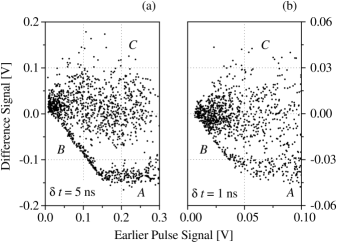
FIG. 4.: DLS plots of background-corrected data from a collapsing SL bubble. Data in (a) is uniformly scaled to account for higher attenuation than in (b). Overall range spanned by the data: (a) 90 ns; (b) 30 ns. The horizontal section A in (a) shows self-similar collapse behavior [27, 32, 20] lasting to within 5 ns of turnaround. The junction between sections A and B appears sharp in (a) but curved in (b), suggesting a smooth turnaround on a $\lesssim 0.5$ ns time scale. A barely resolved kink in section B of (a) might be due to a subnanosecond feature.

In practice, uncertainties in the calibration of the imaging system, as well as in the actual measurement of the bubble size, prompted us to use our measurement of $R_{max}$ as an estimate with $\pm$ 10% uncertainty. The $R(t)$ data were then fed to a fitting algorithm that established $R_{0}$, $P_{a}$, and an appropriate overall scale factor in a nonlinear least-squares calculation using the RPE. The fact that the scale factor for the best fit was determined in this way to be $1.09\pm 0.05$ gave us confidence in the validity of our imaging method. The bubble parameter values thus found were $R_{0}=5.3\pm 0.2~{}\mu$m and $P_{a}=1.34\pm 0.04$ bar.

It is worth mentioning that the time-stamp technique described above can be used directly to obtain light scattering data from a collapsing SL bubble. The drawback is that, unlike in DLS, the electronic response of the measuring instruments is the limiting factor. We used this procedure to collect rough timing information as a cross-check in our analysis of DLS data; with the devices at our disposal, 2-ns resolution was achieved. We estimate that with two microchannel plate PMTs, two constant-fraction discriminators, and a faster TAC, an overall timing uncertainty of 50 ps should be achievable [21].

In Fig. 4 we show representative results from our DLS experiments. In these plots, as in Fig. 1 (b), the abscissa is $I(t_{i})$ and the ordinate is $\delta I_{i}$. In Fig. 4(a) the delay between pulses was 5 ns, and in Fig. 4(b) it was 1 ns. The range of $\delta t$ for which useful information can be gathered is dictated by the physical process under study: delays much shorter than 1 ns yielded DLS plots unresolved into a discernible structure, while delays much longer than 5 ns are not well suited for investigating short time scales.

To aid interpretation, we divide the plots into three regions: A (the collapse, $t<0$), B (the transition region), and C (the rebound, $t>0$). The approximately flat region A corresponds to the collapse, since $\delta I_{i}<0$, indicating that the bubble is shrinking. In C the rebounding bubble expands, but at a much lower rate than during collapse, so $\delta I_{i}$ is positive and smaller in magnitude than in A. However, a greater spread in the data there results in fuzzy clustering across $\delta I_{i}=0$. The straight “wall” in region B forms when the two pulses straddle $t=0$ (compare to the open squares in Fig. 1).

The straight section A in Fig. 4(a) is due to a constant slope of $I(t)$ during collapse. This critical behavior [32, 20] has been previously observed for time scales ranging from 1 $\mu$s to 20 ns prior to turnaround [27]; our observations extend it to $t=-5$ ns. In Fig. 4(a) sections A and B join rather abruptly, indicating a sharp cusp in $I(t)$ on the time scale of the measurement (5 ns). This was expected given the measurements in Ref. [26]. In Fig. 4(b), however, section A appears to show a slight upturn before joining section B, indicating a smooth transition on a time scale less than the pulse delay of 1 ns (since the “wall” section B is still discernible). Scatter in the data prevents a conclusive interpretation, but the available evidence would support an estimate of the bubble turnaround time at a few hundred picoseconds.

The collection lenses used have a f-number of 1.5; the finite acceptance cone they subtend introduces a pollution, or cross talk, of unwanted light from the other pulse in each detector. Because of the strong polarization dependence of scattering, this cross talk is quite small: it was calculated from Mie theory, and confirmed experimentally, to be less than 5% of the total scattered intensity. Electrical cross talk was measured to be less than 5%. The resulting overall intensity uncertainty is therefore around 7%; the difference uncertainty varies across the plot. While in sections A and B the error estimates are consistent with the observed spread in the DLS data, in section C the spread is significantly larger. This has been observed before in Xe-filled bubbles and ascribed to nonsphericity [26]; such asymmetry is reported here as regularly occurring in air-filled bubbles.

In conclusion, we have introduced DLS, a light scattering technique based on the DOG [28] concept of differential measurement and on sensitivity to polarization that uses intense ultrashort laser pulses to bypass the problem of electronic timing jitter. The intensity spread in the data is currently the limiting factor in the resolution achieved with this technique. Effectively, intensity noise is translated into timing noise by the mapping that a DLS plot generates. Accordingly, the resolution in the data shown is approximately 0.5 ns. The intrinsic resolution of DLS, however, is given by the laser pulse width used: with our equipment that can be made as low as 500 fs. Data collected from a collapsing SL bubble confirm earlier findings of a self-similar solution and of subnanosecond turnaround time; our preliminary results suggest that the turnaround is smooth on a time scale of a few hundred picoseconds.

We are very grateful to H. A. Schwettman and the Stanford Picosecond Free Electron Laser Center for supporting this research. We also gratefully acknowledge generous equipment loans by J. R. Willison of Stanford Research Systems. We thank B. P. Barber, B. I. Barker, F. L. Degertekin, R. A. Hiller, G. M. H. Knippels, G. Perçin, S. J. Putterman, C. W. Rella, H. L. Störmer, and members of the Stanford FEL for technical assistance and valuable discussions.

REFERENCES

- [1] Author to whom correspondence should be addressed. Electronic address: gvacca@stanford.edu
- [2] D. F. Gaitan, Ph.D. thesis, University of Mississippi, 1990 (unpublished).
- [3] D. F. Gaitan, L. A. Crum, C. C. Church, and R. A. Roy, J. Acoust. Soc. Am. 91, 3166 (1992).
- [4] D. Lohse et al., Phys. Rev. Lett. 78, 1359 (1997).
- [5] R. G. Holt and D. F. Gaitan, Phys. Rev. Lett. 77, 3791 (1996).
- [6] T. J. Matula and L. A. Crum, Phys. Rev. Lett. 80, 865 (1998).
- [7] J. A. Ketterling and R. E. Apfel, Phys. Rev. Lett. 81, 4991 (1998).
- [8] S. Hilgenfeldt, S. Grossmann, and D. Lohse, Nature (London) 398, 402 (1999).
- [9] M. Dan, J. D. N. Cheeke, and L. Kondic, Phys. Rev. Lett. 83, 1870 (1999).
- [10] V. Q. Vuong, A. J. Szeri, and D. A. Young, Phys. Fluids 11, 10 (1999).
- [11] W. C. Moss, D. A. Young, J. A. Harte, J. L. Levatin, B. F. Rozsnyai, G. B. Zimmerman, and I. H. Zimmerman, Phys. Rev. E 59, 2986 (1999).
- [12] C. Eberlein, Phys. Rev. Lett. 76, 3842 (1996).
- [13] W. Tornow, Phys. Rev. E 53, 5495 (1996).
- [14] A. Prosperetti, J. Acoust. Soc. Am. 101, 2003 (1997).
- [15] T. Lepoint et al., J. Acoust. Soc. Am. 101, 2012 (1997).
- [16] L. Frommhold, Phys. Rev. E 58, 1899 (1998).
- [17] N. García and A. Hasmy, Pis’ma Zh. Éksp. Teor. Fiz. 68, 442 (1998) [JETP Lett. 68, 472 (1998)].
- [18] P. Mohanty and S. V. Khare, Phys. Rev. Lett. 80, 189 (1998).
- [19] J. R. Willison, Phys. Rev. Lett. 81, 5430 (1998).
- [20] A. J. Szeri and B. D. Storey (private communication).
- [21] B. Gompf et al., Phys. Rev. Lett. 79, 1405 (1997).
- [22] R. A. Hiller, S. J. Putterman, and K. R. Weninger, Phys. Rev. Lett. 80, 1090 (1998).
- [23] M. J. Moran and D. Sweider, Phys. Rev. Lett. 80, 4987 (1998).
- [24] R. Pecha et al., Phys. Rev. Lett. 81, 717 (1998).
- [25] W. J. Lentz, A. A. Atchley, and D. F. Gaitan, Appl. Opt. 34, 2648 (1995).
- [26] K. R. Weninger, B. P. Barber, and S. J. Putterman, Phys. Rev. Lett. 78, 1799 (1997).
- [27] G. A. Delgadino and F. J. Bonetto, Phys. Rev. E 56, R6248 (1997).
- [28] C. W. Rella, G. M. H. Knippels, D. V. Palanker, and H. A. Schwettman, Opt. Commun. 157, 335 (1998).
- [29] H. C. van de Hulst, Light Scattering by Small Particles (Dover, New York, 1981), p. 124.
- [30] R. A. Hiller, Ph.D. thesis, University of California at Los Angeles, 1995 (unpublished).
- [31] Y. Tian, J. A. Ketterling, and R. E. Apfel, J. Acoust. Soc. Am. 100, 3976 (1996).
- [32] B. P. Barber et al., Phys. Rep. 281, 65 (1997).