Direct measurement of intersection angle of invariant manifolds for area preserving mappings

Abstract

Intersection angles of stable and unstable manifolds for area preserving mappings are numerically calculated by extremely accurate computation. With the use of multiprecision library the values of angle as small as $10^{-400}$ are obtained. The singular dependence of the angle on the magnitude of hyperbolicity is confirmed. The power-law type prefactor with Stokes constant is also in good agreement with analytical estimation.

1 Introduction

Invariant manifolds are essential components in the phase space structure of Hamiltonian systems. A stable manifold $W^{s}$ and an unstable manifold $W^{u}$ of a fixed point (or a periodic point) is a set of points which asymptotically go to the fixed point as $t\rightarrow\infty$ and $t\rightarrow-\infty$, respectively. These manifolds are invariant with time and are called invariant manifolds.

Suppose we have an integrable Hamiltonian system $H_{0}(I)$ where an unstable manifold is smoothly connected to a stable manifold to form a separatrix. If we perturb the system as $H=H_{0}(I)+\varepsilon H_{1}(I,\varphi)$ then the system is no longer integrable in general and the unstable manifold and stable manifold do not connect smoothly anymore. Rather they intersect transversally and cross each other infinitely many times to produce a complex structure called homoclinic tangle, which eventually gives rise to chaos [LL83, Tab89]. Hence the intersection of invariant manifolds are quite important as the origin of Hamiltonian chaos.

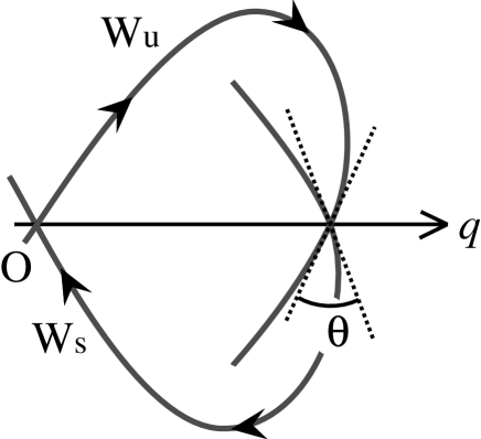
Figure 1: Intersection of unstable and stable manifolds and intersection angle $\theta$. The origin O is a hyperbolic fixed point.

At the point of intersection between $W^{u}$ and $W^{s}$ we can define the “intersection angle” (which is also called as a splitting angle)   $\theta$   between these two manifolds. For several important cases it is estimated to be quite small and behave singularly with respect to the maginitude of hyperbolicity $\varepsilon$ of the fixed point [LST89]. Its leading order behavior for $0<\varepsilon\ll 1$ is

$$\theta=c_{1}\varepsilon^{-\mu}\exp\left(-\frac{c_{2}}{\varepsilon}\right)\ ,$$ (1)

where $c_{1}$, $c_{2}(>0)$ and $\mu(>0)$ are constants. For small values of $\varepsilon$ the exponential factor makes the angle $\theta$ extremely small. Recent asymptotic calculation of functional form of invariant manifolds also contain this singular factor [HM93, TTJ94, TTJ98, NH96, HNK99] thus supporting the estimation.

For area preserving mappings, the area enclosed by an unstable and a stable manifold is equal to the flux from inside to outside (or from outside to inside) of the separatrix per one time step. If the intersection angle gets small so does the area. Hence the smallness of the intersection angle is also important in understanding the global dynamics and relaxation process in Hamiltonian systems.

The singularly smallness of the intersection angle is, however, not yet confirmed thoroughly. Analytical estimation mentioned above is asymptotic approximation, and since it is asymptotic expression for $\varepsilon\rightarrow 0$, we do not know from what value of $\varepsilon$ we can observe the singular behavior.

Usually numerical computation can support analytical estimation. However, ordinary numerical computation is useless in this case to check the singular behavior because of limited precision. Suppose we would like to confirm the proportionality of intersection angle as $\exp(-\pi^{2}/\varepsilon)$. If $\varepsilon=0.1$ the factor is about $\exp(-100)\sim 10^{-43}$. Let us write the normalized tangent vector and their components for stable and unstable manifolds as $\vec{t}^{s}=(\alpha,\beta)$ and $\vec{t}^{u}=(\alpha+d\alpha,\beta+d\beta)$ respectively, and the intersection angle as $\theta$. Then $|d\alpha|=|\beta\theta|$ and $|d\beta|=|\alpha\theta|$ up to the first order of $\theta$. Hence if the angle is of the order of $10^{-40}$ then the differences between values of the components of two vectors $\vec{t}^{s}$ and $\vec{t}^{u}$ are far beyond the range of ordinary double precision of 64-bit, where mantissa (fractional part) is at most 16 decimal digits.

There are two methods which we may use for problems which require extremely high precision. One is “validated computation” [NY98] and the other is “multiprecision”. “Validated computation” is a method to obtain rigorous results with numerical computation. It is based on operation for intervals rather than for numbers. Usual numerical computation on real numbers says e.g., $x=0.123$, but this just mean that the value of $x$ will be near 0.123 and it does not mean that the value of $x$ is exactly 0.123. On the other hand, with the use of validated computation we can rigorously say that the value of $x$ satisfies , for example, $0.122<x<0.124$.

Although validated computation is a powerful tool, it seems not to be all-purpose, and it seems to take time to reformulate the problem one want to solve to fit validated computation. Hence we adopt the second tool, multiprecision library.

In usual numerical computation the precision of variables are uniquely defined in each implementation of language (C, FORTRAN, etc.). On the other hand, using multiprecision library users can define the precision of variables arbitrarily. For various multiprecision tools see the hfloat web page [Arn99]. Here we adopt a multiprecision library called cln [Hai99] which can be used in C++.

The purpose of this paper is (i) to numerically confirm the singular dependence of the intersection angle using multiprecision library, (ii) to find the range of $\varepsilon$ where the singular dependence appears.

There have been several attempts to numerically compute the singular behavior of the intersection angle. In the paper  [LST89] Lazutkin et al. cites a numerical result by C. Simó as private communication and writes that the value of the angle by their analytical estimation is “in good accordance with numerical data”. Also in [ACKRK92], Amick et al. computed the splitting distance of manifolds for a 4th order map $x_{t+3}=x_{t}+\varepsilon g(x_{t+2})$, $g(x)\equiv x(1-x)$ with ordinary double precision. In this paper, we give a refined and concrete result for these pioneering work, by performing direct computation with multiprecision,

This paper is organised as follows. In section 2 we introduce symplectic mappings for which we calculate the intersection angles. In section 3 we describe the method of computation, and the result is presented in section 4. In section 5 we give summary and discussions.

2 Models

The first model we use is a “double-well map”;

$$\phi_{\rm dw}\,:\,(q,p)\mapsto(q^{\prime},p^{\prime})\ ,\ p^{\prime}=p-\varepsilon(2q^{3}-q)\ ,\ q^{\prime}=q+\varepsilon p^{\prime}\ .$$ (2)

This map has a hyperbolic fixed point at (0,0).

For this mapping the intersection angle is estimated to be [NH96]

$$\theta_{\rm dw}=\frac{c_{\rm dw}}{\varepsilon^{5}}\exp\left(-\frac{\pi^{2}}{\varepsilon}\right)\ ,\ c_{\rm dw}=5.00\times 10^{4}\ ,$$ (3)

after change of coordinate.

The second model is the well-known standard map [Chi79];

$$\phi_{\rm st}\,:\,(q,p)\mapsto(q^{\prime},p^{\prime})\ ,\ p^{\prime}=p+\frac{K}{2\pi}\sin(2\pi q)\ ,\ q^{\prime}=q+p^{\prime}\ .$$ (4)

This map has hyperbolic fixed points at $(n,0)$ ($n$ : integer). For standard map the intersection angle is estimated to be  [LST89]

$$\theta_{\rm st}=\frac{c_{\rm st}}{K}\exp\left(-\frac{\pi^{2}}{\sqrt{K}}\right)\ ,\ c_{\rm st}=1118.827706...\ .$$ (5)

3 Method of calculation

Here we describe the method of calculation of intersection angle for the double well map (2). The method for standard map is similar.

In short, we choose two approximate points $P_{\pm}$ for an intersection point, and approximate the intersection angle by the ones between the two manifolds which are on $P_{\pm}$.

3.1 finding an interval which contains PIP

First we search for an intersection point of $W^{u}$ and $W^{s}$. Following an argument similar to [GLS94], it is easily shown that one of the intersection points called principal intersection point (PIP) is on the $q$-axis.

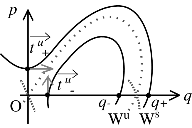
Figure 2: True stable and unstable manifolds (dashed lines) and approximate manifolds (solid lines) and tangent vectors

Suppose we choose an initial point on $q$-axis and update the point backward in time. If the point is near but not on the stable manifold it will approach to the hyperbolic fixed point and then goes away from it. The direction the point goes away shows whether the initial point is on the right or left of the true intersection point. Hence we can set an interval on $q$-axis which include the intersection point between the stable and unstable manifolds.

Then we make the interval narrower by bisection. We call the final interval as $(q_{-},q_{+})$. In actual calculation we set the final width of the interval as

$$|q_{+}-q_{-}|=10^{-100}\ \ \text{for}\ \varepsilon\geq 0.02$$ (6)

and

$$|q_{+}-q_{-}|=10^{-800}\ \ \text{for}\ \varepsilon=0.01$$ (7)

We will use the points $(q_{-},0)$ and $(q_{+},0)$ as approximations for the intersection point and denote as $P_{-}$ and $P_{+}$ respectively, i.e.,

$$P_{\pm}\equiv(q_{\pm},0)$$ (8)

3.2 construction of tangent vectors in the linear region

Now we are going to make tangent vectors at these approximate points $P_{\pm}$.

Although we do not know directly the tangent vectors at $P_{\pm}$, we can calculate them from the linear neighbourhood around the hyperbolic fixed point $(0,0)$.

First we update the points $P_{\pm}$ forward or backward in time;

$$P^{u}_{\pm}\equiv\phi_{\rm dw}^{-N_{u}}\,\left(P_{\pm}\right),\ \ P^{s}_{\pm}\equiv\phi_{\rm dw}^{N_{s}}\,\left(P_{\pm}\right)\$$ (9)

where the time steps $N_{u}$ and $N_{s}$ are sufficiently large for $|P^{u}_{\pm}|\ll 1$ and $|P^{s}_{\pm}|\ll 1$. In actual calculation we determined $N_{u}$ and $N_{s}$ so that $P^{u}_{\pm}$ and $P^{s}_{\pm}$ be the points which are nearest to the hyperbolic fixed point (0,0) on the orbits $\phi_{\rm dw}^{-n}\left(P_{\pm}\right)$ and $\phi_{\rm dw}^{n}\left(P_{\pm}\right)$, respectively.

Since the points $P^{u}_{\pm}$ and $P^{s}_{\pm}$ are quite near to the fixed point (0,0) the map $\phi_{\rm dw}$ can be approximated by its linearized map;

$$\phi_{\rm dw}(q,p)=D\phi_{\rm dw}(0,0)\begin{pmatrix}q\\ p\end{pmatrix}+O(q^{2},p^{2})\ .$$ (10)

Hence the tangent vector of the manifolds which passes $P^{u}$ or $P^{s}$ can be approximated by the invariant curve of the linearized map $D\phi(0,0)$, that is, hyperbola. If we denote

$$D\phi_{\rm dw}=\begin{pmatrix}a+d&c+b\\ c-b&a-d\end{pmatrix}$$ (11)

Then the curve

$$\Phi(q,p)\equiv(b-c)q^{2}+2dqp+(b+c)p^{2}=\text{const.}$$ (12)

is invariant under $\phi_{\rm dw}$  [Gre68]. Hence we can obtain the tangent vector $\overrightarrow{t^{u}}$ and $\overrightarrow{t^{s}}$ of unstable and stable manifolds as the tangent vector of the hyperbola (12)

$$\overrightarrow{t^{\gamma}}_{\pm}\equiv\vec{t}(P^{\gamma}_{\pm})={}^{t}\left(-\frac{\partial\Phi}{\partial p},\,\frac{\partial\Phi}{\partial q}\right)(P^{\gamma}_{\pm})\ ,\gamma=u\ \mbox{or}\ s\ .$$ (13)

3.3 calculation of intersection angles

The tangent vectors at approximate intersection point $P_{\pm}$ is obtained by pulling back the tangent vectors $\vec{t^{u}}$, $\vec{t^{s}}$ to the points $P_{\pm}$ as

$$\overrightarrow{v^{u}}_{\pm}=D\phi^{N_{u}}\left(\overrightarrow{t^{u}}_{\pm}\right)\ ,\ \overrightarrow{v^{s}}_{\pm}=D\phi^{-N_{s}}\left(\overrightarrow{t^{s}}_{\pm}\right)\ .\$$ (14)

Approximation values for intersection angle $\theta$ at each approximate intersection point $P_{\pm}$ is obtained as

$$\cos\theta_{\pm}=\frac{\overrightarrow{v^{u}}_{\pm}\cdot\overrightarrow{v^{s}}_{\pm}}{\left|\overrightarrow{v^{u}}_{\pm}\right|\left|\overrightarrow{v^{s}}_{\pm}\right|}\ .$$ (15)

4 Results

Now we present the results. Computation is performed on a Pentium-II processor PC with Linux operating system (Vine Linux 1.0b) with GNU C/C++ compiler g++ 2.7.2.3 and egcs 1.0.3-release, and the version of multiprecision library is cln 1.0.1. The computation time is typically several hundred times longer than ordinary numerical computation with double precision.

The result for double well map (2) is summarised in the Table 1 and Fig.3. Calculation is performed with 1000 decimal digits for $\varepsilon\geq 0.02$ and 4000 digits for $\varepsilon=0.01$.

$\varepsilon$	$\theta_{-}/\pi$	$\theta_{+}/\pi$
0.6	0.00620123	0.00620123
0.4	2.03305e-05	2.03305e-05
0.2	1.61224e-14	1.61224e-14
0.1	2.0686e-34	2.0686e-34
0.08	1.23026e-44	1.23026e-44
0.06	7.24697e-62	7.24697e-62
0.04	1.06168e-96	1.06168e-96
0.02	2.58525e-202	2.38495e-202
0.01	1.16442e-414	1.16442e-414

Table 1: Intersection angle $\theta$ for double well map. 1000 decimal digits for $\varepsilon\geq 0.02$ and 4000 decimal digits for $\varepsilon=0.01$. $|q_{L}-q_{R}|=10^{-100}$ for $\varepsilon\geq 0.02$ and $10^{-800}$ for $\varepsilon=0.01$ .

Figure 3: Intersection angle for double well map (2). Values are in Table1. The dotted line represents analytical estimation for the singular behavior $\exp(-\pi^{2}/\varepsilon)$(eq.(3)).

.

Here we can see that our numerical results agree quite well with the estimation (eq.(3)). It is clear that the data cannot be fitted by power law. Also we note that the singular have behavior appears for the value of $\varepsilon$ as large as $\varepsilon=0.1$.

The difference of the values between $\theta_{-}$ and $\theta_{+}$ is an indicator of error. Table 1 shows the error is small.

Next we see the results for standard map (4). For standard map we have the principal intersection point on the line $q=\pi$ [GLS94], hence we take its approximation points as $P_{\pm}=(\pi,p_{\pm})$. Calculation is performed with 1000 decimal digits. For standard map in the notation (4) the parameter $\varepsilon$ is equal to $\sqrt{K}$.

$K$	$\theta_{-}/\pi$	$\theta_{+}/\pi$
1.5	0.0692401	0.0692401
1.0	0.0250374	0.0250374
0.8	0.0114877	0.0114877
0.4	0.000324148	0.000324148
0.2	1.16407e-06	1.16407e-06
0.1	2.6934e-10	2.6934e-10
0.08	8.60911e-12	8.60911e-12
0.04	9.47743e-18	9.47743e-18
0.02	2.58424e-26	2.58424e-26
0.01	1.46928e-38	1.46928e-38
0.008	1.60962e-43	1.60962e-43
0.004	4.59792e-63	4.59792e-63
0.002	7.84703e-91	7.84703e-91
0.001	3.14686e-130	3.14686e-130

Table 2: Intersection angle for standard map. 1000 decimal digits are used. $|p_{+}-p_{-}|=10^{-100}$.

Figure 4: Intersection angle for standard map. Values are in Table 2. The dotted line represents analytical estimation for the singular behavior $\exp(-\pi^{2}/\sqrt{K})$ (eq.(5)).

From the figure 4 again we see that the intersection angles agree quite well with analytical estimation (5). Note that we apparently have agreement even above the $K_{c}$, where the last KAM torus is broken and the phase space has global chaotic sea.

Finally we show the prefactors of the singular behavior ($\displaystyle c_{1}\varepsilon^{-\mu}$ in eq.(1).) Here we examine whether the prefactor is in fact a power law type with previously estimated exponent $\mu$. Also the value of the constant $c_{1}$ is interesting to check, because $c_{1}$ contains a constant called Stokes constant, which represents the change in the form of asymptotic expansion of the manifolds[HM93, TTJ94, TTJ98, HNK99, NH96].

Figure 5: Prefactor of intersection angle for double-well map (2). Dashed line represents a least square fitting of the data for $0.01\leq\varepsilon\leq 0.1$, and dotted line represents an analytical estimation $\displaystyle c_{\rm dw}/\varepsilon^{5}$ (3).

Figure 6: Prefactor of intersection angle of standard map. Dashed line represents a least square fitting of the data for $0.001\leq K\leq 0.1$ , and dotted line represents an analytical estimation $\displaystyle c_{\rm st}/K$  (5).

Fig. 5 shows the $\varepsilon$ dependence of the value $\displaystyle\theta\exp(\pi^{2}/\varepsilon)$. Here we see a clear power-law dependence for small values of $\varepsilon$. A least square fitting for $0.01\leq\varepsilon\leq 0.1$ gives

$$\theta\cdot\exp(\pi^{2}/\varepsilon)=41894.5/\varepsilon^{5.04935}\ ,$$ (16)

which is in good agreement with the estimation (3). The difference in the exponent ( 5.04935 for our numerical result and 5 for [NH96] ) is negligible. Also the prefactor 41894.5 is in good agreement with the estimated value of $5.00\times 10^{4}$.

Fig. 6 is for the standard map, where we see a fitting for $0.001\leq K\leq 0.1$

$$\theta/\pi\exp(\pi^{2}/\sqrt{K})=924.551/K^{1.02875}\ ,$$ (17)

again in good agreement with the estimation (5). The difference between our numerical result and the estimation is negligible, as shown in the figure.

5 Summary and discussion

In this paper we have numerically computed the intersection angles between stable and unstable manifolds for two area preserving mappings. Computation is performed with extremely high precision ( with 1000 or 4000 decimal digits) with the use of multiprecision library cln to obtain the angle as small as $10^{-400}$. The singular behavior previously obtained by analytical estimation is confirmed. Hence we have confirmed that the singular small behavior of the intersection angle $\theta\propto\exp(-c/\varepsilon)$ indeed exists for area preserving mappings. Thus the flux in the phase space is quite small for small values of $\varepsilon$, which will make the relaxation process quite slow. In addition, although the analytical estimation is obtained as the asymptotic approximation formula for $\varepsilon\rightarrow 0$ , our numerical results show that the singular dependence appears from rather large value of $\varepsilon$.

Also we have measured the prefactor of the singular factor, and confirmed that the analytical estimations for prefactors are correct. Exponent of the power law is in almost perfect agreement. It appears constants in the prefactors slightly differ from the ones in analytical estimation. This does not necessarily imply that the estimation need to be refined. For the analytical estimation contains a free parameter called switching function $S(0)$ which take a value between 0 and 1[NH96]. Although the estimation is given for $S(0)=1/2$, $S(0)$ can be some other value. In fact [NH96] takes the value $S(0)=0.3$ when comparing their functional form of unstable manifold with numerically obtained orbit. Note that within the range of parameters computed the constant factor do not appear to depend on $\varepsilon$ or $K$.

The singularly smallness of intersection angle was one of several things in the study of Hamiltonian chaos which are predicted but not yet confirmed precisely. Among others are Nekhoroshev bound [Nek77, LN92] and Arnold diffusion [Arn64]. In both cases singular factor appears and it is believed that the singular behavior accounts for slow motion in high-dimensional nearly integrable Hamiltonian systems [KK90]. Extreme precision computation using multiprecision library will reveal some new properties about the slow dynamics of high-dimensional Hamiltonian systems.

6 Acknowledgement

We would like to thank Kazuhiro Nozaki, Yoshihiro Hirata and the members of R-Lab., Nagoya University for stimulating discussions and valuable comments. Thanks are also due to Bruno Haible, the author of the multiprecision libary cln.

References

- [ACKRK92] C. Amick, E. S. C. Ching, L. P. Kadanoff, and V. Rom-Kedar. Beyond all orders: Singular perturbations in a mapping. J. Nonlinear Sci., 2:9–67, 1992.
- [Arn64] V.I. Arnold. Instability of dynamical systems with several degrees of freedom. Sov. Math. Dokl., 5:581, 1964.
- [Arn99] Jorg Arndt. hfloat a c++ library for high precision compuations. http://www.jjj.de/hfloat/, 1997,1999.
- [Chi79] B. V. Chirikov. A universal instability of many-dimensional oscillator systems. Phys. Rep., 52:265 – 379, 1979.
- [GLS94] V. G. Gelfreich, V. F. Lazutkin, and N. V. Svanidze. A refined formula for separatrix splitting for the standard map. Physica, D 71:82–101, 1994.
- [Gre68] M. S. Greene. J. Math. Phys., 27:760, 1968.
- [Hai99] Bruno Haible. CLN, a Class Library for Numbers. http://clisp.cons.org/~haible/packages-cln.html, 1995,1999.
- [HM93] Vincent Hakim and Kirone Mallick. Exponentially small splitting of separatrices, matching in the complex plane and Borel summation. Nonlinearity, 6:57–70, 1993.
- [HNK99] Yoshihiro Hirata, Kazuhiro Nozaki, and Tetsuro Konishi. Exponentially small oscillation of 2-dimensional stable and unstable manifolds in 4-dimensional symplectic mappings. Prog. Theor. Phys., 101:1181–1185, 1999.
- [KK90] T. Konishi and K. Kaneko. Diffusion in Hamiltonian chaos and its size dependence. J. Phys., A 23:L715 – L720, 1990.
- [LL83] A.J. Lichtenberg and M.A. Lieberman. Regular and Stochastic Motion. Springer, Berlin, 1983.
- [LN92] P. Lochak and A. I. Neishtadt. Estimates of stability time for nearly integrable systems with a quasiconvex Hamiltonian. Chaos, 2:495 – 499, 1992.
- [LST89] V. F. Lazutkin, I. G. Schachmannski, and M. B. Tabanov. Splitting of separatrices for standard and semistandard mappings. Physica, D 40:235–248, 1989.
- [Nek77] N.N. Nekhoroshev. An exponential estimate for the stability time of Hamiltonian systems close to integrable ones. Russ. Math. Surv., 32:1–65, 1977.
- [NH96] Katsuhiro Nakamura and Masato Hamada. Asymptotic expansion of homoclinic structures in a symplectic mapping. J. Phys., A 29:7315–7327, 1996.
- [NY98] M. T. Nakao and N. Yamamoto. Validated computation. Nihon Hyouron Sha, (in Japanese), 1998.
- [Tab89] M. Tabor. Chaos and Integrability in Nonlinear Dynamics. John Wiley and Sons, New York, 1989.
- [TTJ94] Alexsander Tobvis, Masa Tsuchiya, and Charles Jaffé. Exponential asymptotic expansions and approximations of the unstable and stable manifolds of the Hénon map. preprint, 1994.
- [TTJ98] Alexsander Tobvis, Masa Tsuchiya, and Charles Jaffé. Exponential asymptotic expansions and approximations of the unstable and stable manifolds of singularly perturbed systems with the Hénon map as an example. Chaos, 8:665–682, 1998.