Semiclassical Gaussian matrix elements for chaotic quantum wells

Abstract

We derive semiclassical expressions for spectra, weighted by matrix elements of a Gaussian observable, relevant to a range of molecular and mesoscopic systems. We apply the formalism to the particular example of the resonant tunneling diode (RTD) in tilted fields. The RTD is a new experimental realization of a mesoscopic system exhibiting a transition to chaos. It has generated much interest and several different semiclassical theories for the RTD have been proposed recently.

Our formalism clarifies the relationship between the different approaches and to previous work on semiclassical theories of matrix elements. We introduce three possible levels of approximation in the application of the stationary phase approximation, depending on typical length scales of oscillations of the semiclassical Green’s function, relative to the degree of localization of the observable. Different types of trajectories (periodic, normal, closed and saddle orbits) are shown to arise from such considerations. We propose a new type of trajectory (“minimal orbits”)and show they provide the best real approximation to the complex saddle points of the stationary phase approximation.

We test the semiclassical formulae on quantum calculations and experimental data. We successfully treat phenomena beyond standard periodic orbit (PO) theory: “ghost regions” where no real PO can be found and regions with contributions from non-isolated POs. We show that the new types of trajectories (saddle and minimal orbits) provide accurate results. We discuss a divergence of the contribution of saddle orbits, which suggests the existence of bifurcation-type phenomena affecting the complex and non-periodic saddle orbits.

I INTRODUCTION

The density of states (DoS): $d(E)=\sum_{i}\delta(E-E_{i})$ of a quantum system -in other words, the density of eigenstates $E_{i}$ at a given energy $E$- plays a key role in the field of “quantum chaos”. Gutzwiller [1] found a semiclassical approximation for the oscillatory part of the DoS, in terms of the periodic orbits of the (chaotic) classical system. However the DoS, generally, is not probed directly in experiments, as they measure an observable $I(E)$. Often the latter can be related to the DoS by a sort of Fermi golden rule:

$$I(E)=\sum_{i}\langle\psi_{i}|\hat{\cal A}|\psi_{i}\rangle\delta(E-E_{i})\quad\mbox{.}\quad$$ (1)

In other words, the measured quantity $I(E)$ is the DoS weighted by the expectation value of an observable $\hat{\cal A}$ over the eigenstate $|\psi_{i}\rangle$ with eigenenergy $E_{i}$.

Experiments probing such a weighted DoS include ,among others, spectroscopic studied of atoms in static fields [2], molecular (Franck-Condon) transitions [3] and electronic transport in microcavities [4]. While the Periodic Orbits (POs) have offered a powerful tool for understanding these experiments, a quantitative analysis requires one to go beyond the Gutzwiller formula. Semiclassical expressions for the “matrix elements” may also be investigated using the stationary phase approximation (SPA).

The first semiclassical approximation for matrix elements [7] involved POs, and in essence reduced to the Gutzwiller trace formula (GTF) of the density of states, weighted by the Wigner transform $A_{W}$ of the observable $\hat{\cal A}$, evaluated along each PO. This result was found by assuming that $A_{W}$ is smooth in phase space, and by neglecting it in the SPA. On the other hand, the photoabsorption rate of the hydrogen atom was expressed in terms of closed orbits (COs) passing through the nucleus [8], because the observable $\hat{\cal A}$ is very localized. Another semiclassical formula, for the conductance fluctuations in microstructures, involved “angle orbits” defined by an angle related to the width of the leads [4].

Hence the the type of contributing trajectories depends strongly on the relative smoothness of $\hat{\cal A}$ and the semiclassical Green’s function used to represent the DoS. Further, the type of semiclassical expressions also depended on the level of approximation used in the SPA integrations. For the semiclassical matrix elements [7], the variations of $A_{W}$ in both the SPA condition and integrations were neglected. A more refined version developed for molecular transitions [13] also neglected them in the SPA condition (which yielded periodic orbits), but included them in the integrations. Finally, “angle orbits” were obtained by considering both the observable and the semiclassical Green’s function when applying the SPA.

A broad range of situations involve Gaussian matrix elements, given by an observable which contains a projector on a Gaussian: molecular excitation from a low vibrational state [13], in the conductance of microcavities with parabolic leads [14] as well as the tunnelling diode experiments which form the subject of the present study. The Gaussian matrix elements, conveniently, yield fairly simple integrals, and also have a very clear localization length scale.

The resonant tunneling diode in tilted fields (RTD) —which is a mesoscopic realization of quantum wells with tunneling barriers— was introduced recently as a new probe of quantum chaos [5, 6]. The oscillations of the measured current (as a function of the applied voltage) were linked to unstable [5] and stable [6] periodic oscillations, following a heuristic application of the Gutzwiller trace formula [1] and taking into account the accessibility of the periodic orbits (POs) to the tunneling electrons.

The RTD experiments generated considerable interest and prompted the development of a series of semiclassical theories. One study proposed two separate formulae (obtained by two different level of approximation in the integrations) using normal orbits starting and finishing perpendicular to the barrier [9]. Another study proposed a formula using periodic orbits [10], similar to the approach of Zobay and Alber [13]. However, it was shown [22] that the normal and periodic orbits could not give satisfactory results in all experimental regimes, and that a new type of complex and non-periodic trajectories (the saddle orbits) [12] provided an accurate semiclassical description. Subsequently, Closed orbits, as well as orbits having a minimum transverse momentum were proposed [11] in order to achieve similar results using only real trajectories. Here we will review and also extend our study of RTD problem, in order to clarify previous work and to prescribe the best semiclassical description for this type of problem.

In section II we derive a general semiclassical expression for Gaussian matrix elements, expressed in terms of an arbitrary type of orbits [eq. (29)]. We outline the RTD experiments and show that they are a realization of Gaussian matrix elements.

In section III we explain different reasonable assumptions one can make regarding the localization of the Gaussian observable in position or phase space. We show that different assumptions yield various types of contributing trajectories (POs, COs, normal orbits, etc.), and correspondingly different expressions for the current formula. We approach the problem from three levels of approximation: $(i)$ no approximation, yielding saddle orbits (SOs); $(ii)$ the intermediate formulae, where we neglect one term in the SPA condition; $(iii)$ the “hard limit” level, where we neglect one term in both the SPA condition and the SPA integrations (for POs, this corresponds to the result of Eckhardt et al.[7]).Our general formula enable us to reproduce easily any of the five semiclassical theories of the current in the RTD that have been proposed in the literature [9, 10, 11, 12]. We also propose a new type of trajectories, we term minimal orbits,selected by requiring that the gradient of the argument of the exponential is minimal (instead of zero as in the standard SPA).

In section IV we test the different formulae against quantum mechanical calculations and experimental results (obtained from Müller et al.[6] and analyzed in [20]). We focus on the most interesting regimes, beyond the scope of standard PO theory: regimes where there is no real contributing PO (“ghost” regions), or where non-isolated POs give non-separable contributions; in these cases the saddle orbits succeed while the PO formula fails. Here we find that the closed orbit formula [11] represents an improvement over the PO formulae, but requires a complicated strategy where one switches between different types of real trajectories in different regimes. On the other hand, the minimal orbits achieve the goal of reproducing the accuracy of the complex SOs —across the whole transition from regularity to chaos— by using only real dynamics. We also investigate bifurcation-type phenomena for saddle orbits, where their contribution peaks sharply, somewhat reminiscent of the effect of bifurcations on the GTF. More detail on this work can be found in [15].

II THEORY: Derivation of general semiclassical formula and the RTD as an example of Gaussian matrix elements

A Semiclassical Gaussian matrix elements

We wish to find a semiclassical approximation to the quantity

$$I(E)=\sum_{i}\langle\psi_{i}|\hat{\cal A}|\psi_{i}\rangle\delta(E-E_{i})=-\frac{1}{\pi}{\rm I}{\rm Im}\>{\rm Trace}\>[\hat{\cal A}\hat{G}]=-\frac{1}{\pi}{\rm I}{\rm Im}\>\int d\mbox{\boldmath$q$}\int d\mbox{\boldmath$q^{\prime}$}{\cal A}(\mbox{\boldmath$q$},\mbox{\boldmath$q^{\prime}$})G(\mbox{\boldmath$q$}^{\prime},\mbox{\boldmath$q$})\quad\mbox{,}\quad$$ (2)

where $|\psi_{i}\rangle$ is an eigenstate of the system with eigenenergy $E_{i}$. We also introduced the position matrix elements of the observable, ${\cal A}(\mbox{\boldmath$q$},\mbox{\boldmath$q^{\prime}$})=\langle\mbox{\boldmath$q$}|\hat{\cal A}|\mbox{\boldmath$q$}^{\prime}\rangle$, and of the energy Green’s function $G(\mbox{\boldmath$q^{\prime}$},\mbox{\boldmath$q$})=\langle\mbox{\boldmath$q^{\prime}$}|\hat{G}|\mbox{\boldmath$q$}\rangle=\lim_{\eta\to 0_{+}}\langle\mbox{\boldmath$q^{\prime}$}|(E+i\eta-\hat{H})^{-1}|\mbox{\boldmath$q$}\rangle$. We consider here a closed system with two degrees of freedom $\mbox{\boldmath$q$}=(x,z)$, and described by a Hamiltonian $\hat{H}$. We consider here the special case of Gaussian matrix elements, i.e., projectors on a Gaussian:

$$\hat{\cal A}=|\Phi\rangle\langle\Phi|\quad\mbox{,}\quad\Phi(x,z)=\phi(z)\chi(x)\quad\mbox{,}\quad\phi(z)=\left(\frac{\beta}{\pi\hbar}\right)^{1/4}e^{\textstyle-\frac{\beta}{2\hbar}z^{2}}\quad\mbox{.}\quad$$ (3)

$\chi(x)$ can also be a Gaussian (in Franck-Condon transitions) or a cut $\delta(x)$ (in microcavities or the RTD). To derive the semiclassical approximation, one proceeds in two steps. First, one uses the semiclassical expression of the Green’s function involving all classically allowed trajectories going from $q$ to $q^{\prime}$ with energy $E$ [1]:

$$G(\mbox{\boldmath$q^{\prime}$},\mbox{\boldmath$q$})\stackrel{{\scriptstyle\hbar\to 0}}{{\simeq}}\frac{2\pi}{(2\pi i\hbar)^{3/2}}\sum_{\mbox{\boldmath$q$}\to\mbox{\boldmath$q^{\prime}$}}\frac{m}{\sqrt{p_{x}p^{\prime}_{x}m_{12}}}e^{iS(\mbox{\boldmath$q$},\mbox{\boldmath$q^{\prime}$})/\hbar}\quad\mbox{,}\quad$$ (4)

where $S$ is the action of the trajectories, $p_{x}$ the momentum in $x$, and $m_{12}=\frac{\partial z^{\prime}}{\partial p_{z}}$. Note that we define our monodromy matrix $M=\partial(z^{\prime},p_{z}^{\prime})/(\partial z,\partial p_{z})$ with respect to $z$ and not to the coordinate perpendicular to the trajectory as usual. We did not include the phase $(-i\mu\pi/2)$ arising from the number $\mu$ of conjugate (or focal) points along the trajectory.

The second step requires the use of the stationary phase approximation (SPA) in eq. (2). This states that an exponential integral can be approximated by a quadratic expansion of the argument of the exponential around the point where the argument is stationary. Depending on the relative smoothness of $\hat{\cal A}$ and $\hat{G}$, different further approximations can be made.

B Description of the RTD

A resonant tunneling diode (RTD) can be constructed by adding different layers of semiconductors and applying a voltage $V$ between the emitter (where the electrons accumulate before entering the well) and the collector. In effect, this will create a wide quantum well between two tunneling barriers (see Fig. 1). One also applies a magnetic field $B$ at tilt angle $\theta$ in the $X-Z$ plane, which creates instability in the classical dynamics in the well.

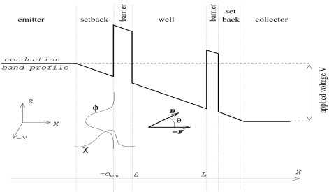
FIG. 1.: Schematic diagram of the RTD. We show the experimental setup (not to scale), with the conduction band profile (effective voltage). Below is the 3-$D$ coordinates axis; the magnetic field $B$ is at tilt angle $\theta$ with the electric field $-\mbox{\boldmath$F$}$ in the $X-Z$ plane. We also show a representation of the distribution of the electrons in the emitter setback: a Gaussian distribution $\phi$ in $Z$ due to the magnetic field $B\cos\theta$, and an Airy function $\chi$ in $X$ due to the triangular well. The width of the well is $L=120\>{\rm nm}=2267\>{\rm a.u.}$.

The Hamiltonian describing the motion of the electrons in the well can be reduced to two dimensions [18, 9] and reads

$$H(\mbox{\boldmath$p$},\mbox{\boldmath$q$})=\frac{1}{2m}(p_{x}^{2}+p_{z}^{2})-Fx+\frac{B^{2}}{2m}(x\sin\theta-z\cos\theta)^{2}\quad\mbox{,}\quad$$ (5)

where we used atomic units ($e=m_{e}=\hbar=1$), $F=V/L$ and the effective mass of the electron is $m=0.067$. The length of the well is $L=120\>{\rm nm}=2267\>{\rm a.u.}$. We consider the barriers to be of infinite height; the classical electrons will undergo specular bounces ($p_{x}\to-p_{x}$) at the barriers ($x=0,L$), while the quantum wave function $\psi_{i}$ of the (isolated) well has vanishing boundary conditions [$\psi_{i}(x=0,z)=\psi_{i}(x=L,z)=0$].

C Bardeen expression for the RTD current

The current $I(E)$ can be calculated using the assumption of weak tunneling across the emitter barrier, the collector playing no important role as all the sites are free for the outgoing electrons (which are accelerated by the voltage drop). In that case one can use the Bardeen [16] formalism, which is a sort of first-order perturbation theory for a high barrier [9]:

$$J = \frac{2\pi}{\hbar}\sum_{i}|{\cal M}_{i}|^{2}\delta(E-E_{i})\quad\mbox{,}\quad{\cal M}_{i}=\frac{\hbar^{2}}{2m}\int d\mbox{\boldmath$q$}\left\{\Phi^{*}(\mbox{\boldmath$q$})\frac{\partial\psi_{i}}{\partial x}(\mbox{\boldmath$q$})-\frac{\partial\Phi^{*}}{\partial x}(\mbox{\boldmath$q$})\psi_{i}(\mbox{\boldmath$q$})\right\}\delta(x)\quad\mbox{,}\quad\mbox{\boldmath$q$}=(x,z)\quad\mbox{.}\quad$$ (6)

In essence, this is an overlap between $\psi_{i}$ and the “initial state” $\Phi$, which is the state of the electron in the emitter region prior to tunneling. The overlap is made on a cut taken on the emitter barrier at $x=0$. It was shown [17] that the use of finite or infinite barriers does not change significantly the important features of the current. Note that the Bardeen expression is formally a matrix element like eq. (2), if one writes ${\cal M}_{i}=i\langle\Theta|\psi_{i}\rangle$ with $|\Theta\rangle=\hbar/(2m)|\big{(}\hat{p}_{x}\hat{\delta}_{x}+\hat{\delta}_{x}\hat{p}_{x}\big{)}\otimes 11_{z}|\Phi\rangle,\quad\hat{\delta}_{x}=|x=0\rangle\langle x=0|.$

In the RTD, one can assume [9] a separable form for $\Phi$: an Airy function $\chi(x)$ induced by the triangular well, and a Landau state $\phi(z)$ induced by the effective magnetic field $\beta:=B\cos\theta$. In the experiments under consideration and for small $\theta$, one can further assume that only the lowest Landau level [eq. (3)] is occupied [5].

It is well known that the imaginary part of the Green’s function can reproduce the sum of the delta functions of the energies, as written in eq. (2). The current is therefore given by

$$J = -\frac{\hbar^{3}}{2m^{2}}{\rm I}{\rm Im}\>\int dz\int dz^{\prime}\left\{\Phi(\mbox{\boldmath$\bar{q}$})\Phi^{*}(\mbox{\boldmath$\bar{q}^{\prime}$})\partial^{2}_{xx^{\prime}}G(\mbox{\boldmath$\bar{q}^{\prime}$},\mbox{\boldmath$\bar{q}$})-\partial_{x}\Phi(\mbox{\boldmath$\bar{q}$})\Phi^{*}(\mbox{\boldmath$\bar{q}^{\prime}$})\partial_{x^{\prime}}G(\mbox{\boldmath$\bar{q}^{\prime}$},\mbox{\boldmath$\bar{q}$})\right.$$ (8)

$$\left.-\Phi(\mbox{\boldmath$\bar{q}$})\partial_{x^{\prime}}\Phi^{*}(\mbox{\boldmath$\bar{q}^{\prime}$})\partial_{x}G(\mbox{\boldmath$\bar{q}^{\prime}$},\mbox{\boldmath$\bar{q}$})+\partial_{x}\Phi(\mbox{\boldmath$\bar{q}$})\partial_{x^{\prime}}\Phi^{*}(\mbox{\boldmath$\bar{q}^{\prime}$})G(\mbox{\boldmath$\bar{q}^{\prime}$},\mbox{\boldmath$\bar{q}$})\right\}\quad\mbox{.}\quad$$

Then one can use the semiclassical expression (4) for the Green’s function. Because of the Bardeen cut, only trajectories going from and to the left barrier $\mbox{\boldmath$\bar{q}$}=(x=0,z)$ can contribute to the current. Note that the derivatives of $\psi_{i}$ in eq. (6) will be transfered to derivatives of the Green’s function, yielding factors $-p_{x}=\partial S/\partial x$ and $p_{x}^{\prime}=\partial S/\partial x^{\prime}$. It has been shown [11, 9] that the Green’s function, as well as its first derivatives, vanish at the hard barrier (this can be understood by the Dirichlet conditions for $\psi_{i}$). Hence only the first term in eq. (8) contributes, and one is left with:

$$J=-\frac{2|\chi(0)|^{2}}{m\sqrt{2\pi\hbar}}{\rm I}{\rm Im}\>i^{-3/2}{\cal I}\quad\mbox{,}\quad{\cal I}=\int dz\int dz^{\prime}\sum_{(x=0,z)\to(x^{\prime}=0,z^{\prime})}\sqrt{\frac{p_{x}p^{\prime}_{x}}{-m_{12}}}\phi(z)\phi^{*}(z^{\prime})e^{iS(x=0,z;x^{\prime}=0,z^{\prime})/\hbar}\quad\mbox{.}\quad$$ (9)

D Derivation of the general semiclassical formula

First we rewrite eq. (9) using the Gaussian form of the initial state:

$${\cal I} = \sqrt{\frac{\beta}{\pi\hbar}}\sum_{\ell}\int\!\!\ \!\!\int_{\Omega_{\ell}}\!\!dz\>dz^{\prime}\sqrt{\frac{p_{x}p^{\prime}_{x}}{-m_{12}}}e^{\varphi(z,z^{\prime})/\hbar}\quad\mbox{with}\quad\varphi(z,z^{\prime}):=iS(z,z^{\prime})-\frac{\beta}{2}(z^{2}+z^{\prime 2})\quad\mbox{.}\quad$$ (10)

We have also taken the sum over trajectories $(x=0,z)\to(x^{\prime}=0,z^{\prime})$ outside the integrals where it becomes a sum over all the different “families” $\{\ell\}$ of trajectories existing in a domain $\{(z,z^{\prime})\in\Omega_{\ell}\}$.

The tool used for this kind of integration is the stationary phase approximation (SPA). Briefly, it states that only trajectories $z_{0}\to z_{0}^{\prime}$ having a stationary phase [$\partial\varphi(z_{0},z_{0}^{\prime})/\partial z=\partial\varphi(z_{0},z_{0}^{\prime})/\partial z^{\prime}=0$] contribute to the integrals, all the others being either damped by the Gaussian or destroyed by the random cancellations of the oscillations due to the action. Then one has to expand the phase quadratically around the contributing type of orbit and integrate, pushing the limit of the integration $\Omega\to{\rm I}{\rm R}^{2}$.

We saw in the introduction that a variety of contributing orbits have been proposed in the case of the RTD. Therefore, we shall not specify the type of orbits yet, but rather develop a general formula valid for any type, and discuss the different choices in section III.

One can relate the second derivatives of the action to the monodromy matrix $M$ [1], and the quadratic expansion of the action reads:

$$S(z,z^{\prime}) \simeq S(z_{0},z^{\prime}_{0})+\delta z\frac{\partial S}{\partial z}(z_{0},z^{\prime}_{0})+\delta z^{\prime}\frac{\partial S}{\partial z^{\prime}}(z_{0},z^{\prime}_{0})$$ (12)

$$+\frac{1}{2}\left[\delta z^{2}\frac{\partial^{2}S}{\partial z^{2}}(z_{0},z^{\prime}_{0})+2\delta z\delta z^{\prime}\frac{\partial^{2}S}{\partial z\partial z^{\prime}}(z_{0},z^{\prime}_{0})+\delta z^{\prime 2}\frac{\partial^{2}S}{\partial z^{\prime 2}}(z_{0},z^{\prime}_{0})\right]$$

$$= S_{0}-p^{0}_{z}\delta z+p^{0}_{z^{\prime}}\delta z^{\prime}+\frac{1}{2m_{12}}\left[\delta z^{2}m_{11}-2\delta z\delta z^{\prime}+\delta z^{\prime 2}m_{22}\right]$$ (13)

$$=: {\cal S}_{2}(\delta z,\delta z^{\prime};z_{0},z^{\prime}_{0})\quad\mbox{,}\quad$$ (14)

with $\delta z=z-z_{0}$ and $\delta z^{\prime}=z^{\prime}-z_{0}^{\prime}$. The “phase” of the initial state is already quadratic. We follow the techniques of Bogomolny and Rouben [9], and complete the square:

$${\cal I} \stackrel{{\scriptstyle\rm SPA}}{{\simeq}}\sqrt{\frac{\beta}{\pi\hbar}}\sum_{\ell_{0}}\int_{{\rm I}{\rm R}^{2}}d\mbox{\boldmath$\gamma$}\sqrt{\frac{p_{x}p^{\prime}_{x}}{-m_{12}}}e^{\varphi_{2}(\mbox{\boldmath$\gamma$})/\hbar}$$ (15)

$$\varphi_{2}(\mbox{\boldmath$\gamma$}) :=i{\cal S}_{2}(\mbox{\boldmath$\gamma$};z_{0},z^{\prime}_{0})-\frac{\beta}{2}(z^{2}+z^{\prime 2})$$ (18)

$$\stackrel{{\scriptstyle(\ref{quadaction})}}{{=}}iS_{0}-\frac{\beta}{2}(z_{0}^{2}+z_{0}^{\prime 2})+\mbox{\boldmath$\xi$}^{\rm T}\mbox{\boldmath$\gamma$}+\frac{1}{2}\mbox{\boldmath$\gamma$}^{\rm T}{\cal H}\mbox{\boldmath$\gamma$}$$

$$=iS_{0}-\frac{\beta}{2}(z_{0}^{2}+z_{0}^{\prime 2})-\frac{1}{2}\mbox{\boldmath$\xi$}^{\rm T}{\cal H}^{-1}\mbox{\boldmath$\xi$}+\frac{1}{2}(\mbox{\boldmath$\gamma$}+\mbox{\boldmath$\gamma$}_{1})^{\rm T}{\cal H}(\mbox{\boldmath$\gamma$}+\mbox{\boldmath$\gamma$}_{1})$$

with

$$\mbox{\boldmath$\gamma$}=(\delta z,\delta z^{\prime})=(z-z_{0},z^{\prime}-z^{\prime}_{0})\quad\mbox{,}\quad$$ (19)

$$\mbox{\boldmath$\xi$}=(-\beta z_{0}-ip_{z}^{0},-\beta z^{\prime}_{0}+ip_{z^{\prime}}^{0})\quad\mbox{,}\quad\mbox{\boldmath$\gamma$}_{1}={\cal H}^{-1}\mbox{\boldmath$\xi$}\quad\mbox{,}\quad$$ (20)

$${\cal H}=\left(\begin{array}[]{cc}\displaystyle-\beta+i\frac{m_{11}}{m_{12}}&\displaystyle-i\frac{1}{m_{12}}\\ \\ \displaystyle-i\frac{1}{m_{12}}&\displaystyle-\beta+i\frac{m_{22}}{m_{12}}\end{array}\right)\quad\mbox{.}\quad$$ (24)

$\ell_{0}$ denotes the different contributing trajectories. With the change of variables $\mbox{\boldmath$\gamma^{\prime}$}=\mbox{\boldmath$\gamma$}+\mbox{\boldmath$\gamma$}_{1}$, the last term in eq. (18) gives a pure two-dimensional Gaussian, equal to $2\pi\hbar/\sqrt{\det{\cal H}}$. The final result is

$${\cal I}=\sum_{\ell_{0}\atop(z_{0}\to z^{\prime}_{0})}2\sqrt{\frac{\beta\pi\hbar p_{x}p_{x}^{\prime}}{-\cal D}}e^{\left[iS_{0}+\Gamma(z_{0},z^{\prime}_{0})\right]/\hbar}\quad\mbox{,}\quad$$ (25)

with

$${\cal D} = -m_{21}-i\beta{\rm Tr}M+\beta^{2}m_{12}$$ (26)

$$\Gamma(z,z^{\prime}) = -\frac{\beta}{2{\cal D}}\times\Bigg{\{}z^{2}\left[-m_{21}-i\beta m_{11}\right]+z^{\prime 2}\left[-m_{21}-i\beta m_{22}\right]+2i\beta zz^{\prime}$$ (27)

$$+ \frac{1}{\beta^{2}}p_{z}^{2}\left[-i\beta m_{22}+\beta^{2}m_{12}\right]+\frac{1}{\beta^{2}}p_{z^{\prime}}^{2}\left[-i\beta m_{11}+\beta^{2}m_{12}\right]+2i\frac{1}{\beta}p_{z}p_{z^{\prime}}$$ (28)

$$+ 2\frac{i}{\beta}zp_{z}\left[i\beta m_{22}-\beta^{2}m_{12}\right]+2\frac{i}{\beta}z^{\prime}p_{z^{\prime}}\left[-i\beta m_{11}+\beta^{2}m_{12}\right]+2zp_{z^{\prime}}-2z^{\prime}p_{z}\Bigg{\}}\>\quad\mbox{.}\quad$$ (29)

The above formula describes the oscillatory part of the current. We do not consider here the “smooth” part, obtained by considering zero-length trajectories [9]; this part varies slowly with the energy, and corresponds to the Weyl term in Gutzwiller’s theory of the density of states [1].

The loss of coherence due to phonon scattering is not considered in the formalism presented here. It can be modeled by adding an exponential factor $\exp(-T/\tau)$ in the sum, where $T$ is the real part of the total time of each trajectory and $\tau$ is the damping (decoherence) time. We shall proceed the other way round, canceling the effects of the damping in the experiments.

The formula is valid only for isolated expansion orbits. Also, we did not write explicitly the phase arising from the number $\mu$ of conjugate points along the trajectory, as we shall primarily consider individual contributions from isolated trajectories.

III THEORY: Semiclassical formulae for specific types of trajectories

At this stage one should go back to the SPA applied to eq. (10), and examine which choices of expansion orbits have been or can be made. First we mention one remarkable feature of the RTD, which is that for any starting $z$, there exists, generically, a starting momentum $\check{p}_{z}$ for which the trajectory is a time-reversed duplicate of itself and therefore closed. We call such trajectories time-symmetric (TS). They are defined by

$${\rm\bf TS}\>:\quad(z,\check{p}_{z})\to(z^{\prime},p_{z}^{\prime})=(z,-\check{p}_{z})$$ (30)

and satisfy the important relation $m_{11}=m_{22}$. The existence of TS orbits is a consequence of the fact that for any starting $z$, one can find a starting $p_{z}$ so that there is either a perpendicular bounce on a wall [$p_{z}(x=0\>{\rm or}\>L)=0$], or a turning point on the energy surface at a point where $\mbox{\boldmath$p$}=0$. Note that some self-retracing trajectories with $p_{z}^{0}\neq 0$ or $z^{\prime}\neq z$ are not TS.

One actually finds that each choice of expansion orbit shown below contains a subset which is time-symmetric (TS), and that in almost all cases only the TS subset contribute to the current. This is the reason why we first write (29) for time-symmetric (TS) orbits. Using (30) and $m_{11}=m_{22}$, one finds

$$\Gamma_{\rm TS}(z_{0})=-\frac{\beta}{1-\delta}\Bigg{\{}z_{0}^{2}-\left[\frac{1}{\beta^{2}}(p_{z}^{0})^{2}-2\frac{i}{\beta}z_{0}p_{z}^{0}\right]\delta\Bigg{\}}$$ (31)

where we have defined

$$\quad\delta=-i\beta\frac{m_{12}}{m_{11}-1}\quad\mbox{.}\quad$$ (32)

We now consider different possible choices for the expansion points.

A Saddle orbits (SOs)

The first expansion orbits we consider here are given by the strict application of the stationary phase condition on (10):

$${\rm\bf SO}\>:\quad\left\{\begin{array}[]{ll}&p_{z}^{0}=i\beta z_{0}\\ &p_{z^{\prime}}^{0}=-i\beta z^{\prime}_{0}\quad\mbox{.}\end{array}\right.$$ (33)

We call such trajectories saddle orbits (SOs) [12]. Inserting eq. (33) in eq. (29), one finds $\Gamma_{\rm SO}(z_{0},z^{\prime}_{0})=-\frac{\beta}{2}\left(z_{0}^{2}+z_{0}^{{}^{\prime}2}\right)$, i.e.

$${\cal I}_{\rm SO}=\sum_{{\rm SOs}\atop(z_{0}\to z^{\prime}_{0})}2\pi\hbar\sqrt{\frac{p_{x}p_{x}^{\prime}}{-\cal D}}e^{iS_{0}/\hbar}\phi(z_{0})\phi(z_{0}^{\prime})\quad\mbox{.}\quad$$ (34)

In the case where SOs are TS (TSSOs) one has $\Gamma_{\rm TSSO}(z_{0})=-\beta z_{0}^{2}$. We shall show in section IV that the SOs are the most successful types of orbits for a semiclassical description of the quantum current. One difficulty with SOs is the fact that they are complex. This is the reason why Bogomolny and Rouben[9] decided to avoid them (and considered real trajectories), although they were well aware of the fact that the stationary phase approximation yields SOs.

The SOs are non-periodic; this means that one cannot look at repetitions of a “primitive” SO, as it would not satisfy the SO condition. Instead one must search for an SO with a higher period. Contrary to complex POs, the complex conjugate of an SO is not an SO.

B Normal orbits (NOs)

To obtain real trajectories, one has to make a further approximation and neglect one term in the SPA condition (33). Bogomolny and Rouben [9] considered that the dynamics in the well are very chaotic; in that case one should expect the oscillations due to the action to dominate the Gaussian damping of the initial state. Formally, this corresponds to taking the limit $\beta\to 0$ in (33), and yields normal orbits (NOs):

$${\rm\bf NO}\>:\quad\left\{\begin{array}[]{ll}&p_{z}^{0}=0\\ &p_{z^{\prime}}^{0}=0\quad\mbox{.}\end{array}\right.$$ (35)

Essentially, this states that the contributing trajectories are determined solely by the oscillations of the Green’s function: they must cancel the variations of the action, however small their accessibility to the initial state is. Moreover, TS normal orbits (TSNOs) have $z_{0}^{\prime}=z_{0}$. This implies that TSNOs are actually a special subset of periodic orbits, that are time-symmetric (TSPO) and start with $p_{z}$=0. In the non-TS case ($z_{0}^{\prime}\neq z_{0}$), the second repetition of the NO is actually a TSPO; the first repetition of a non-TS NO is in a sense a “half PO”. One finds

$$\Gamma_{\rm NO}(z_{0},z^{\prime}_{0})=-\frac{\beta}{2{\cal D}}\Bigg{\{}z_{0}^{2}\left[-m_{21}-i\beta m_{11}\right]+(z_{0}^{\prime})^{2}\left[-m_{21}-i\beta m_{22}\right]+2i\beta z_{0}z^{\prime}_{0}\Bigg{\}}\quad\mbox{,}\quad$$ (36)

which is equation (109) of Bogomolny and Rouben(1999) [9]. In the TS case, one has $\Gamma_{\rm TSNO}(z_{0})=-\frac{\beta}{1-\delta}z_{0}^{2}$, and the current can be written

$${\cal I}_{\rm TSNO}=\sum_{{\rm NOs}\atop(z_{0}\to z^{\prime}_{0})}2\sqrt{\frac{\beta\pi\hbar p_{x}p_{x}^{\prime}}{-|{\cal D}|}}e^{-\beta z_{0}^{2}\left(1-\gamma\right)/\hbar}e^{i(S+\Delta S-\arg{\cal D}/2)/\hbar}\quad\mbox{,}\quad\gamma=\frac{|\delta|^{2}}{1+|\delta|^{2}}\quad\mbox{,}\quad\Delta S=\beta z_{0}^{2}\frac{|\delta|}{1+|\delta|^{2}}\quad\mbox{.}\quad$$ (37)

We shall call this expression the PO/NO formula. Note the shift $\Delta S$ of the frequency of the oscillations from the action $S$ of the PO. Also, the term $\gamma$ can reduce the Gaussian damping due to the initial state, for trajectories with large $z_{0}$. In fact, this formula takes into account torus quantization effects à la Miller [19] occurring in large islands of stability surrounding stable POs. It has been shown [9] that it is analytically equivalent to a model [20] building the current as an overlap between the initial Gaussian and the wavefunction in the well approximated by the harmonic oscillator state corresponding to Miller tori.

It is also interesting to consider the case when $\beta$ is very small. The first terms of an expansion of $\Gamma$ and ${\cal D}$ in powers of $\beta$ yield

$${\cal D}_{\rm HLNO}\to-m_{21}\quad\mbox{,}\quad\Gamma_{\rm HLNO}\to-\frac{\beta}{2}\left[z_{0}^{2}+(z_{0}^{\prime})^{2}\right]\quad\Rightarrow\quad{\cal I}_{\rm HLNO}=\sum_{{\rm NOs}\atop(z_{0}\to z^{\prime}_{0})}2\pi\hbar\sqrt{\frac{p_{x}p_{x}^{\prime}}{m_{21}}}e^{iS/\hbar}\phi(z_{0})\phi(z_{0}^{\prime})$$ (38)

We refer to this kind of expansion as “hard limit” (HL). This was the first formula proposed by Bogomolny and Rouben[9]. It is justified in the case of extremely chaotic dynamics, where the oscillations of the Green’s function are supposed to be much stronger than the Gaussian decay of the initial state. In the case of a TS orbit, the precise condition for the validity of this theory is [9]

$$\frac{\left|\frac{\partial^{2}S}{\partial z^{2}}\right|}{\beta}=\left|\frac{m_{11}-1}{\beta m_{12}}\right|=\frac{1}{\left|\delta\right|}\gg 1\quad\mbox{.}\quad$$ (39)

The HL result corresponds to the SPA method applied to the Green’s function only. As $\beta$ is supposed to be very small, the initial state function is neglected in the integrations (15), and is taken out of them; it is evaluated at the NO and gives the simple Gaussian factor $\Gamma_{\rm HL}$. The integral is carried out only over the Green’s function, bringing in a prefactor $m_{21}$ and the exponential of the pure action. Note that this is the usual way of proceeding with the SPA method, while considering the variation of both functions in the integral (15) is not standard.

C Central closed orbits (CCOs)

Narimanov and Stone[11] proposed a semiclassical approach which effectively amounts to consideration of the other extreme case, where the Gaussian damping dominates the action oscillations; this assumption can be justified for fairly regular dynamics. This corresponds to taking the limit $\beta\to\infty$ in (33), and yields central closed orbits (CCOs):

$${\rm\bf CCO}\>:\quad\left\{\begin{array}[]{ll}&z_{0}=0\\ &z^{\prime}_{0}=0\quad\mbox{.}\end{array}\right.$$ (40)

Here the contributing trajectories give maximal accessibility to the initial state, while they do not cancel the variations of the action. In this case one finds

$$\Gamma_{\rm CCO}(p_{z}^{0},p_{z^{\prime}}^{0})=-\frac{1}{2\beta{\cal D}}\Bigg{\{}(p_{z}^{0})^{2}\left[-i\beta m_{22}+\beta^{2}m_{12}\right]+(p_{z^{\prime}}^{0})^{2}\left[-i\beta m_{11}+\beta^{2}m_{12}\right]+2i\beta p_{z}^{0}p_{z^{\prime}}^{0}\Bigg{\}}\quad\mbox{.}\quad$$ (41)

This formula is equivalent to equation (14) of Narimanov and Stone[11]. (They derived a general formula for any number of excited Landau levels in the initial state.) TS central closed orbits (TSCCOs) have $p_{z^{\prime}}^{0}=-p_{z}^{0}$, and give $\Gamma_{\rm TSCCO}(z_{0})=\frac{1}{\beta}\frac{\delta}{1-\delta}(p_{z}^{0})^{2}$.

One can also consider the hard limit, i.e. the first order expansion in ${\cal O}(1/\beta)$:

$${\cal D}_{\rm HLCCO}\to\beta^{2}m_{12}\quad\mbox{,}\quad\Gamma_{\rm HLCCO}\to-\frac{1}{2\beta}\left[(p_{z}^{0})^{2}+(p_{z^{\prime}}^{0})^{2}\right]\quad\Rightarrow\quad{\cal I}_{\rm HLCCO}=\sum_{{\rm CCOs}\atop(z_{0}\to z^{\prime}_{0})}2\pi\hbar\sqrt{\frac{p_{x}p_{x}^{\prime}}{-m_{12}}}e^{iS/\hbar}\tilde{\phi}(p_{z}^{0})\tilde{\phi}(p_{z^{\prime}}^{0})\quad\mbox{.}\quad$$ (42)

Here we introduced the initial state (i.e., the observable) in momentum representation: $\tilde{\phi}(p_{z})=(\beta\pi\hbar)^{-1/4}\exp[-p_{z}^{2}/(2\beta\hbar)]$. The hard limit is equivalent to neglecting the quadratic term of the action in the integral (15). The integration of the linear term with the initial state is in effect a Fourier transform, and brings in the value of the initial state in momentum representation at the CCO. Alternatively, one can express the Green’s function and the initial state in momentum representation, and argue that the latter is smooth and can be taken out of the integral by stationary phase approximation. A similar expression in terms of “closed orbits at the nucleus” and involving a weighting by $m_{12}^{-1/2}$ was found in the semiclassical theory of the photoabsorption spectra of a hydrogen atom in external fields [8]. The similarity is somewhat limited, as the expression for the photoabsorption spectra is much more complicated than mere momentum wave functions (it involves matching the semiclassical Green’s function to a quantum one in the vicinity of the nucleus).

D Periodic orbits (POs)

Periodic orbits are a natural choice, as it follows the expansion around POs found in the derivation of the Gutziller trace formula for the density of states. A discussion of this choice is more adequately made using a phase space formalism, described in appendix A. Alternatively, a more direct route is to define “average-difference” coordinates

$$\left\{\begin{array}[]{ll}&\bar{z}=\frac{1}{2}(z^{\prime}+z)\\ &\Delta z=z^{\prime}-z\end{array}\right.\quad\mbox{,}\quad\left\{\begin{array}[]{ll}&\bar{p_{z}}=\frac{1}{2}(p_{z}^{\prime}+p_{z})\\ &\Delta p_{z}=p_{z}^{\prime}-p_{z}\end{array}\right.\quad\mbox{,}\quad$$ (43)

which one uses to write the $z$-observable $\hat{A}=|\phi\rangle\langle\phi|$ in position space as:

$$\bar{A}(\bar{z},\Delta z)=\phi(\bar{z}-\frac{1}{2}\Delta z)\phi^{*}(\bar{z}+\frac{1}{2}\Delta z)=\sqrt{\frac{\beta_{\bar{z}}^{1/2}\beta_{\Delta z}^{1/2}}{\pi\hbar}}e^{\textstyle-\frac{\beta_{\bar{z}}}{\hbar}\bar{z}^{2}-\frac{\beta_{\Delta z}}{4\hbar}\Delta z^{2}}\quad\mbox{,}\quad$$ (44)

while the Wigner transform is defined by

$$W(\bar{z},\bar{p}_{z})=\frac{1}{2\pi\hbar}\int d\Delta z\>e^{i\bar{p}_{z}\Delta z/\hbar}\bar{A}(\bar{z},\Delta z)=\frac{1}{\pi\hbar}e^{\textstyle-\frac{\beta_{\bar{z}}}{\hbar}\bar{z}^{2}-\frac{1}{\beta_{\Delta z}\hbar}\bar{p}^{2}}\quad\mbox{.}\quad$$ (45)

Here we have written two different Gaussian widths $\beta_{\bar{z}}$ and $\beta_{\Delta z}$ for respectively $\bar{z}$ and $\Delta z$. Of course in reality we have $\beta_{\bar{z}}=\beta_{\Delta z}=\beta$, but retaining the distinction clarifies the following discussion. The action is $\bar{S}(\bar{z},\Delta z)=S(\bar{z}-\Delta z/2,\bar{z}+\Delta/2)$, and its quadratic expansion around a point $(\bar{z}_{0},\Delta z_{0})$ reads:

$$\bar{{\cal S}}_{2}(\bar{z},\Delta z) = \bar{S}_{0}+\Delta p_{z}^{0}\delta\bar{z}+\bar{p}_{z}^{0}\delta\Delta z$$ (46)

$$+ \frac{1}{2m_{12}}\left[\delta\bar{z}^{2}({\rm Tr}M-2)+\delta\bar{z}\delta\Delta z(m_{22}-m_{11})+\frac{1}{4}\delta\Delta z^{2}({\rm Tr}M+2)\right]\quad\mbox{}\quad$$ (47)

with $\delta\bar{z}=\bar{z}-\bar{z}_{0}$ and $\delta\Delta z=\Delta z-\Delta z_{0}$.

The idea is to apply the SPA method to the integral ${\cal I}\propto\int\Delta z\int\bar{z}\>\bar{A}(\bar{z},\Delta z)\exp[i\bar{{\cal S}}_{2}(\bar{z},\Delta z)/\hbar]$, i.e., with respect to the variables (43). The SPA condition reads:

$$\left\{\begin{array}[]{ll}&\bar{p}_{z}^{0}=-\frac{1}{2}i\beta_{\Delta z}\Delta z_{0}\\ &\Delta p_{z}^{0}=-2i\beta_{\bar{z}}\bar{z}_{0}\quad\mbox{.}\end{array}\right.$$ (48)

In Eckhardt et al.[7], one assumes the Wigner transform to be smooth as a function of $(\bar{z},\bar{p}_{z})$. This corresponds to the case $\beta_{\bar{z}}\to 0$ and $\beta_{\Delta z}\to\infty$, which gives for (48):

$${\rm\bf POs}\>:\quad\left\{\begin{array}[]{ll}&\Delta z_{0}=0\\ &\Delta p_{z}^{0}=0\quad\mbox{,}\end{array}\right.$$ (49)

that is, periodic orbits (POs). Hence POs arise naturally when one consider a smooth Wigner transform; as $\bar{A}(\bar{z},\Delta z)$ is its Fourier transform [see eq. (A1)], it is smooth in $\bar{z}$, but localized in $\Delta z$. This corresponds to a “local” operator, in the sense that $\bar{A}(\bar{z},\Delta z)\sim\bar{a}(\bar{z})\delta(\Delta z)$. This also enables one to recover the Gutzwiller trace formula, via $\hat{A}\to 11\Rightarrow\bar{A}(\bar{z},\Delta z)\to\delta(\Delta z)$.

Things are different for the Gaussian matrix elements, which are written as a projector over a Gaussian state. They are the product of two functions depending separately on $z$ and $z^{\prime}$, and cannot have the property of being simultaneously smooth in $\bar{z}$ and localized in $\Delta z$: either it is localized in both, or it is smooth in both. One cannot change $\beta_{\bar{z}}$ and $\beta_{\Delta z}$ independently. This fact was noted by Zobay and Alber [13] in their work on Franck-Condon molecular transitions, which involved very similar equations.

Nevertheless, it is still fruitful to consider periodic orbits for the RTD. Putting $z^{\prime}=z,p_{z}^{\prime}=p_{z}$ in (29), one finds

$$\Gamma_{\rm PO}(z^{0},p_{z}^{0}) = -\frac{\beta}{2{\cal D}}\Bigg{\{}z_{0}^{2}\left[-2m_{21}-i\beta({\rm Tr}M-2)\right]+\frac{1}{\beta^{2}}(p_{z}^{0})^{2}\left[-i\beta({\rm Tr}M-2)+2\beta^{2}m_{12}\right]$$ (51)

$$\hskip 56.9055pt-2z_{0}p_{z}^{0}\left[m_{22}-m_{11}\right]\Bigg{\}}\quad\mbox{.}\quad$$

This formula is equivalent to equation (19) of Narimanov and Stone[11]. An important subset of POs are TS, and have $p_{z}^{0}=0$ (TSPOs). As mentioned above, TSPOs are identical to TSNOs, and therefore give the same contribution (37).

For the hard limit, an expansion in $\beta_{\bar{z}}$ and $1/\beta_{\Delta z}$ gives

$${\cal D}_{\rm HLPO}\to\beta({\rm Tr}M-2)/2i\quad\mbox{,}\quad\Gamma_{\rm HLPO}\to-\beta_{\bar{z}}\bar{z}_{0}^{2}-\frac{1}{\beta_{\Delta z}}(\bar{p}_{z}^{0})^{2}\quad\Rightarrow\quad{\cal I}_{\rm HLPO}=\sum_{{\rm POs}\atop(z_{0}\to z^{\prime}_{0})}2\pi\hbar\sqrt{\frac{2\pi i\hbar p_{x}p_{x}^{\prime}}{{\rm Tr}M-2}}e^{iS/\hbar}W(\bar{z_{0}},\bar{p}_{z}^{0})\quad\mbox{.}\quad$$ (52)

This corresponds to the formula for semiclassical matrix elements proposed in Eckhardt et al.[7], that was derived for an observable which is smooth in phase space. This formula is basically the Gutzwiller trace formula (GTF) weighted by the Wigner transform calculated for each PO. To get the hard limit directly from the integration (15), one neglects the quadratic variation of $S$ due to $\Delta z$ , and neglects the variations of $e^{-\beta\bar{z}^{2}/\hbar}$ over the integral (i.e., one uses its value at the PO). The integration of $e^{-\beta\Delta z^{2}/(4\hbar)}$ with the linear term in $S$ due to $\Delta z$ is a Fourier transform, which gives the Wigner part $e^{-(\bar{p}_{z}^{0})^{2}/(\beta\hbar)}$. The integration over the variations of the action due to $\bar{z}$ gives the ${\rm Tr}M-2$ prefactor, as in the GTF. Alternatively, one can work in phase space and apply the SPA to (A3), neglecting the variations of the Wigner function $W$ in the integral. Note finally that the hard limit formula for POs expresses in some sense the heuristic approach that was first used to interpret semiclassically the current in the RTD, where one considered the effects of the stability of POs on the density of states given by the GTF, while taking into account the accessibility of the PO to the tunneling electrons [5, 6].

E Minimal orbits (MOs)

Narimanov and Stone[11] proposed the CCOs in order to extend the PO formula to regions where one has no real POs (also called “ghost regions”, see section IV), while avoiding the problem of complex dynamics raised by SOs. They also proposed an extension of the CCO formula in terms of time-symmetric orbits which had a minimal momentum transfer $\Delta p_{z}=-2p_{z}$, i.e., $\partial(\Delta p_{z})/\partial z=0$. The argument was that the Wigner transform in the PO formula has a Gaussian damping that kills the contribution of trajectories with $p_{z}$ that are not small. This is the only proposed semiclassical formula for the RTD that we have not tested by comparison with quantum calculations. Instead, we will propose and test another formula which is based on a similar idea.

The SPA method applied on (10) prescribes finding an expansion point which makes the function $\varphi_{2}(z,z^{\prime})$ stationary. This can be achieved if one can find a point $(z_{0},z^{\prime}_{0})$ such that the linear term $\mbox{\boldmath$\xi$}^{\rm T}\mbox{\boldmath$\gamma$}$ in (18) vanishes for all $\mbox{\boldmath$\gamma$}=(z-z_{0},z^{\prime}-z^{\prime}_{0})$, i.e., $\mbox{\boldmath$\xi$}(z_{0},z^{\prime}_{0})=(-\beta z_{0}-ip_{z}^{0},-\beta z^{\prime}_{0}+ip_{z^{\prime}}^{0})=(0,0)$. As already mentioned, this requires complex trajectories (the SOs). The idea here is to find the real trajectory which minimizes $\mbox{\boldmath$\xi$}^{\rm T}(z_{0},z^{\prime}_{0})$ and therefore should gives the minimal linear term in (18). This is in some sense the best real approximation of the complex saddle point. Defining

$${\cal L}(z,z^{\prime})=\left|\mbox{\boldmath$\xi$}^{\rm T}\mbox{\boldmath$\xi$}(z,z^{\prime})\right|^{2}=\beta^{2}\left[z^{2}+z^{\prime 2}\right]+p_{z}^{2}+p_{z^{\prime}}^{2}\quad\mbox{,}\quad$$ (53)

one will look for

$$0 = \frac{1}{2}\frac{\partial\cal L}{\partial z}=\beta^{2}z-\frac{p_{z}m_{11}+p_{z}^{\prime}}{m_{12}}$$ (54)

$$0 = \frac{1}{2}\frac{\partial\cal L}{\partial z^{\prime}}=\beta^{2}z^{\prime}+\frac{p_{z}+p_{z}^{\prime}m_{22}}{m_{12}}\quad\mbox{.}\quad$$ (55)

This prescription defines minimal orbits (MOs):

$${\rm\bf MO}\>:\quad\left\{\begin{array}[]{ll}\displaystyle&z^{\prime}_{0}=-m_{22}z_{0}+\frac{m_{21}}{\beta^{2}}p_{z}^{0}\\ \displaystyle&p_{z^{\prime}}^{0}=\beta^{2}m_{12}z_{0}-m_{11}p_{z}^{0}\quad\mbox{.}\end{array}\right.$$ (56)

The contribution of MOs to the current will be given by using (29) with the $\{z_{0},p_{z}^{0};z^{\prime}_{0},p_{z^{\prime}}^{0}\}$ of the MO. Again, one finds that the most important MOs are TS. TSMOs have $p_{z}^{0}=z_{0}\beta^{2}\frac{m_{12}}{m_{11}-1}=z_{0}\beta|\delta|$. Their contribution will be calculated with (31).

F Summary of the formulae

For the sake of completeness, we mention here the last possibility for neglecting one element in (33). One considers the case of a Wigner transform that is very localized in $\bar{z}$ and $\bar{p}_{z}$. This corresponds to $\beta_{\bar{z}}\to\infty$ and $\beta_{\Delta z}\to 0$, which gives for (48):

$${\rm\bf AO}\>:\quad\left\{\begin{array}[]{ll}&\bar{z}_{0}=0\\ &\bar{p}_{z}^{0}=0\quad\mbox{.}\end{array}\right.$$ (57)

We call such trajectories average orbits (AOs), but shall not write nor study their contribution. It is interesting to note that for TSAOs, one has $z_{0}=z_{0}^{\prime}=0$, which means that TSAOs are identical to TSCCOs.

We show in Fig. 2 a schematic representation of the different orbits and their related formulae. We classify them according to the level of approximation of the SPA method used in the Gaussian integrations, that is: $(i)$ no approximation, which gives the saddle orbits (SOs) and the related formula eq. (34); $(ii$) approximation in the SPA condition (but none in the integration), which gives the normal [NO, eq. (37)], central closed [CCO, eq. (41)], periodic [PO, eq. (51)] or average (AO) orbits [and their related formulae]; $(iii)$ approximation in both the SPA condition and integrations, which give the hard limit formula (HLPO, HLNO, HLCCO). Then we classify them according to the underlying hypotheses regarding the predominance of the Green’s function $\hat{G}$ or the observable $\hat{A}$ in determining the contributing trajectories. This is linked to their relative smoothness in position or phase space. Note that the SOs correspond in this classification to the angle orbits found for the conductance of microcavities [4], in the sense that both types of orbits are derived without any approximation of the SPA condition.

FIG. 2.: Schematic representation of the different semiclassical formulae. The vertical axis describes the three different levels of approximation: one can neglect one function ($A$ or $G$) in the saddle point condition [COND], also in the integrations [COND + INT], or in none [NONE]. The horizontal plane describes the relative localization/oscillations length scales of $\hat{A}$ and $\hat{G}$ (e.g., the left end means that the oscillations of $\hat{G}$ in position space are on a much smaller scale than the localization of $\hat{A}$, etc.).

IV Comparison between semiclassical results and quantum calculations and experiments;analysis of results.

A Scaling the classical dynamics

In our comparisons between classical/semiclassical/quantal dynamics we exploit an important property of the RTD : its Hamiltonian can be scaled with respect to the magnetic field [21]. Then, the classical dynamics depends only on the ratio $\epsilon=F/B^{2}$ instead of the independent values of $F$ and $B$ (the ratio $R=E/V$ is roughly constant in the experiments) . The experimental regime [6] corresponds to the interval $1000<\epsilon<100000$. The classical dynamics in this range evolve from chaotic (low $\epsilon$) to regular dynamics (high $\epsilon$) [20]. It is preferable to scale the action not with respect to $B$, but rather with respect the action of the $\theta=0^{\circ},B=0,R\gg 1$ problem: $S_{0}\simeq 2L\sqrt{2mV(R+1/2)}$. In this integrable case, the number of oscillations of the wave function approximated by the WKB method [1] is given by

$${\cal N}:=\frac{S_{0}}{2\pi}=\frac{L}{\pi}\sqrt{2mV(R+1/2)}\quad\mbox{,}\quad$$ (58)

which we shall consider as a measure of the “effective $\hbar^{-1}$” in the general case as well. We define the scaled action by $\hat{S}(\epsilon):=S/S_{0}$. This definition is convenient as the three types of experimental oscillations [6] then correspond to trajectories with $\hat{S}\simeq 1,2$ or $3$. We term these period-one, period-two and period-three trajectories respectively. Also, $\hat{S}$ depends only on $\epsilon$, but is roughly constant as $\epsilon$ varies. We called the important period-one trajectories $t$ and the most important primitive period-two trajectories $s$ [20].

We can obtain the period of the voltage oscillations generated by a given trajectory. The frequency of the oscillations of the semiclassical current is given by the imaginary part of the argument of the exponential in eq. (25): $\Sigma={\rm I}{\rm Re}\>S+{\rm I}{\rm Im}\>\Gamma$. We can also define its scaled version $\hat{\Sigma}=\Sigma/2\pi{\cal N}$. Then one has two consecutive maxima $\{V,V+\Delta V\}$ in the current-voltage trace (neglecting the variation of $\arg{\cal D}$) when

$$2\pi=\Sigma(V+\Delta V)-\Sigma(V)=\Delta[\Sigma]=\Delta\left[2\pi\hat{\Sigma}(\epsilon){\cal N}(V)\right]=2\pi\hat{\Sigma}\frac{\cal N}{2V}\Delta V\quad\Rightarrow\quad\Delta V=\frac{2V}{{\cal N}\hat{\Sigma}}\quad\mbox{.}\quad$$ (59)

This can be contrasted to the heuristic interpretation based on the DoS that was used before [5, 6], where the voltage oscillations were directly obtained from the energy oscillations given by the GTF: $\Delta V=\Delta E/R=2\pi\hbar/RT$, where $T$ is the period of the contributing PO. This relation is not exactly correct for two reasons: the current oscillations are not given by the action $S$ but by $\Sigma$, and the period $T$ arises in the GTF from $\partial S(E,B,V)/\partial E=T$ taken at constant $B$ and $V$, while in our case $V$ varies with $E$ through the constant $R$.

B The different types of orbits

Because of the decoherence induced by phonon scattering, only the shortest trajectories contribute to the current in the RTD we analyzed (which has a width $L=120\>{\rm nm}=2267\>{\rm a.u.}$). We compare in Fig. 3 the shape of the different types of contributing (all of the $t$-type). Examples of plots of the other important class of orbits, the $s$-type orbits may be found elsewhere eg  [12, 11]. In (a) we present the traversing periodic orbit (PO) $t_{0}$, which makes one bounce on each wall, and is responsible for the broad experimental voltage oscillations [20, 5]. It is perpendicular on the left wall ($p_{z}^{0}=0$), and is therefore time-symmetric (TS) and also a TS normal orbit (NO). There are two period-two POs, born in two pitchfork bifurcations around $\epsilon=13000$. $t_{v}$ is self-retracing but non-perpendicular; hence it is not TS: reversing the momentum at the end of the trajectory (on the left wall), one does not find oneself on the portion of the trajectory on which the orbit started. $t_{u}$ is TS and therefore also a TS NO; there is also another non-TS NO hidden: it is “half” the PO $(z_{0}=-80\to z_{0}^{\prime}=550)$ and will be denoted by $t_{u}\!-\!\!NO$.

As $\epsilon$ decreases towards the chaotic regime, $t_{0}$ disappears with an unstable partner $t_{0}^{-}$ in a tangent bifurcation at $\epsilon=6500$. They are replaced by a pair of POs which are complex conjugates of each other; the one giving a physical contribution is called “ghost” and is denoted by $t_{\rm gh}$. At $\epsilon=3000$ (b), a new real PO $t_{1}$ has appeared. We also show the saddle orbit (SO) and minimal orbit (MO) that are related to the $t$-type trajectories; they do not disappear in any bifurcations and are linked to all the three POs ($t_{0},t_{\rm gh}$) and $t_{1}$ as $\epsilon$ decreases. In this region the SO and MO are between $t_{\rm gh}$ and $t_{1}$.

In (c) we illustrate the non-periodicity of SOs. We show $t_{0}\!-\!\!SO$, related to the primitive PO $t_{0}$, and the very different $2t_{0}\!-\!\!SO$, that is related to the second repetition of the PO. Because SOs (as well as MOs and CCOs) are not periodic, one cannot continue the propagation of a primitive orbit, but one has to look for another orbit with the adequate action, period and number of bounces so that it corresponds to the repetition of a primitive PO. Note that in some cases (e.g., $t_{0}\!-\!\!SO$ at $\theta=27^{\circ},\epsilon<17000$), one cannot find an SO corresponding to the second repetition of a PO, although one has the SO linked to the primitive PO.

FIG. 3.: Shape of different types of orbits of the $t$-type at $\theta=11^{\circ}$. The right wall is at $x=L=120\>{\rm nm}=2267\>{\rm a.u.}$. For complex trajectories, we show the real part $({\rm I}{\rm Re}\>x,{\rm I}{\rm Re}\>z)$. (a) $\epsilon=14000$; the periodic orbit (PO) $t_{v}$ is self-retracing but not time-symmetric (TS), as it not perpendicular on the left wall ($p_{z}^{0}\neq 0$); $t_{0}$ and $t_{u}$ are TS POs and therefore also TS NOs; the “half PO” $t_{u}\!-\!\!NO$ $(z_{0}=-80\to z_{0}^{\prime}=550)$ is a non-TS normal orbit (NO). (b) $\epsilon=3000$; here we have the complex ghost $t_{\rm gh}$ which has appeared in the tangent bifurcation of $t_{0}\!-\!\!PO$ at $\epsilon=6500$; we show the related saddle orbit $t_{0}\!-\!\!SO$ and minimal orbit $t_{0}\!-\!\!MO$; we also have a real PO $t_{1}$. (c) $\epsilon=18000$; we show the saddle orbit $t_{0}\!-\!\!SO$ corresponding to the primitive $t_{0}\!-\!\!PO$, as well as the saddle orbit $2t_{0}\!-\!\!SO$ corresponding to the second repetition of the PO. (d) $\epsilon=10000$; the central closed orbit $t_{0}\!-\!\!CCO$ is defined by $z_{0}=0$.

An example of a central closed orbit (CCO) is shown in (d): it looks very different from the related PO.

C $\theta=11^{\circ}$ theory and experiments: ghost regions and torus quantization

The method used to compare semiclassical, quantum and experimental results was explained by Saraga and Monteiro[20]. For each $\epsilon$, we generate a scaled quantum (QM) and semiclassical current that oscillates with ${\cal N}$, in the range $12<{\cal N}<42$ ,corresponding to the experimental $B$ range read at constant $V=0.5\>{\rm V}$. We Fourier transform the current with respect to the pair ${\cal N},\hat{S}$ and get a power spectrum that has peaks at certain values of the action. The height of the peaks gives the amplitude of the oscillation, while their position indicates their type: period-one oscillations when $\hat{S}\simeq 1$, period-two when $\hat{S}\simeq 2$, etc. For the experiments, we read the amplitude of the oscillations directly from $I-V$ traces provided by G Boebinger [6], that we analyzed and presented in [20]. We correct the experimental $\epsilon$ by $30\%$ to take into account effect of the voltage dependence of the mass. To allow for damping due to phonon scattering, we scale the amplitudes by $\exp[T/\tau]$, where $T$ is the (real part of the) total time of the contributing classical orbit and $\tau\sim 0.1\>{\rm ps}$ [5] is a decoherence time. We use here the value $\tau\simeq 0.115\>{\rm ps}$ estimated by comparing the maximal values of the quantum and experimental amplitudes. We normalize all amplitudes to the amplitudes at $\theta=0^{\circ}$, where for the semiclassics we have $\Gamma=0$ and $|{\cal D}(\theta=0^{\circ})|=2B,\forall\epsilon$.

Fig. 4 presents the amplitudes of the different semiclassical formulae at $\theta=11^{\circ}$. Here we study period-one oscillations, which correspond to the broad voltage oscillations seen in the experiments[6] and called “$t$” series [5]. They arise from trajectories making one bounce on each wall; ( the $t_{0}$ orbit at high $\epsilon$ and $t_{1}$ at low $\epsilon$).

In (a) we see that the quantum calculation based on the Bardeen model reproduces quantitatively the experimental behaviour, over a large range of parameters (corresponding to $3\>{\rm T}<B<12\>{\rm T}$). We did not read experimental amplitudes for $\epsilon>25000$, because of the presence of period-two oscillations.

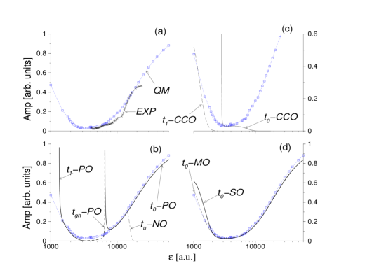
FIG. 4.: Amplitude of the semiclassical formulae for period-one oscillations at $\theta=11^{\circ}$, compared with quantum mechanical calculations [QM, dotted line with squares] as the dynamical parameter $\epsilon$ varies. (a) Comparison between experimental results [EXP] and quantum mechanical results [QM]. (b)Quantal results and semiclassical results for the PO/NO formula, to which three POs contribute: $t_{0}$, the complex ghost $t_{\rm gh}$ and $t_{1}$. We also show the contribution of $t_{u}\!-\!\!NO$, which is not a PO. (c) Quantal results and the semiclassical CCO formula. (d) Quantal results and the semiclassical SO and MO formulae. The figure shows that while both the SO and the MO formulae give good agreement over the whole range, the PO/NO/CCO formulae give agreement only over a partial range.

The periodic orbit theory is compared to quantum calculations in (b). For $t_{0},t_{\rm gh}$ and $t_{1}$ we use the PO/NO formula (37), which is the common formula given by POs and NOs. The semiclassical formula is accurate in both the chaotic ($\epsilon<3000$) and regular ($\epsilon>10000$) regions. In the latter, the semiclassical contribution can be understood by Miller torus quantization [19]. The large stable island of $t_{0}$ supports quantum states that are approximately harmonic oscillators (HO) functions in the plane perpendicular to the orbit; this will be discussed in more detail below. We also see that the contribution of $t_{u}\!-\!\!NO$ to the NO formula seems unrelated to the quantum behavior. Note the spike at $\epsilon=6500$; this corresponds to the tangent bifurcation where $t_{0}$ and $t_{0}^{-}$ disappear. It is not a divergence, as the complex ${\cal D}$ does not vanish. The spike is due to the rapid variation of $\Gamma$ near the bifurcation.

The most interesting region is $3000<\epsilon<6500$, where there is no real contributing PO (the “ghost” region). We included the contribution of the complex ghost PO $t_{\rm gh}$, but we see that its contribution is too small [22]. A detailed view is shown in Fig. 5 (a). There we see that the ghost contribution is too small by roughly a factor three compared to the QM results. The saddle orbit (SO), on the other hand, describes accurately the QM amplitudes all across the tangent bifurcation, the ghost region and the region where $t_{1}\!-\!\!PO$ takes over [see also Fig. 4 (d)]. Finally, we see in Fig. 5 (a) that the unstable partners of the tangent bifurcations $t_{0}^{-}$ and $t_{1}^{-}$ do not contribute to the current. This is a general feature that we observed at any angle $\theta$: only a very small subset of trajectories give a significant semiclassical contribution. A study of the amplitudes of period-two oscillation (not shown here) shows that other POs like $t_{v}$ and $t_{u}$ are not related to the QM results although their contribution to the PO/NO formula is significant.

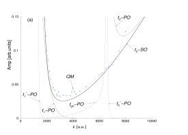
FIG. 5.: (a) Details of the period-one amplitudes at $\theta=11^{\circ}$ in the low $\epsilon$ region. This is the region where no real PO exist, and where the contribution from the complex ghost PO $t_{\rm gh}$ is too small, while the SO contribution is accurate and joins up the contribution from the POs $t_{0}$ and $t_{1}$. We also show the contribution of the unstable POs $t_{0}^{-}$ and $t_{1}^{-}$, which are not seen in the QM behaviour. (b) Comparison of experimental voltage periods (line with crosses) with the semiclassical period generated by the SO $t_{0}$ (solid line).

The contributions of central closed orbits (CCOs) are shown in Fig. 4 (c). The main objective of the CCO theory as presented by Narimanov and Stone[11] was to complement their PO theory in the absence of real PO (the “ghost” region). It partially succeeds, as its amplitude for $3000<\epsilon<5000$ corresponds to the quantum one. However, it is clearly inaccurate for $\epsilon>5000$ and gets worse in the regular region, where one could have expected the assumptions underlying the theory to be respected (in this regular regime, the oscillations of the Green’s function should be smooth compared to the localization of the initial state). Similarly, the CCO theory is not very accurate in the chaotic region (low $\epsilon$).

We show in (d) the result of the saddle (SO) and minimal orbit (MO) formulae. There is only one SO and one MO corresponding to the three POs $t_{0},t_{\rm gh}$ and $t_{1}$. Both theories are very accurate and reproduce the quantum amplitudes across the whole transition from regular to chaotic dynamics. Actually, the MO contribution is even more precise than the SO at very low $\epsilon$.

Finally, we study in Fig. 5 (b) the frequencies of the oscillations via their voltage period $\Delta V$. We show the semiclassical period calculated with eq. (59) from the saddle orbit $t_{0}$. We do not show quantum periods, which are accurately described by the semiclassics. The theoretical periods underestimate the experimental values by some $10\%$. This however is a confirmation of the fact that $t_{0}$ orbits are indeed linked to the broad experimental oscillations.

Torus quantization is illustrated in Fig. 6, where we present Wigner and wave functions of quantum states contributing to the current. The wave functions are approximately separable into a HO state and a WKB-type wave function along the trajectory. ${\cal N}_{i}$ gives roughly the number of longitudinal oscillations, while the number of perpendicular oscillations corresponds to the pseudo quantum number $k$ of the HO state. One can use this assumption to build a current as the overlap between the initial state and the HO state [20]. This is valid for stable POs, and it has been shown to be equivalent to the PO [10] and NO [9] formula in the case of time-symmetric orbits. The Wigner distributions show the ring structure associated with HO states.

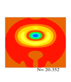
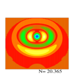
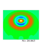
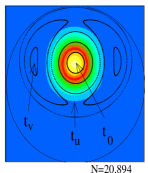
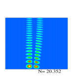
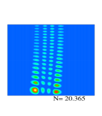
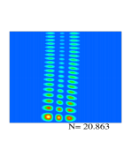
FIG. 6.: Quantum state contributing to the current in the torus quantization regime at $\theta=11^{\circ},\epsilon=15000$, labelled by their eigenvalue ${\cal N}_{i}$ . For the Wigner distributions on the emitter barrier (top row), the vertical axis is $z$ and the horizontal axis is $-p_{z}$; the range is adapted to the size of the (classically allowed) surface of section. For the wave functions (bottom rows) the vertical axis is $x\in[0,L=2267]\>{\rm a.u.}$ and the horizontal axis is $-z\in[-2000,2000]\>{\rm a.u.}$. For ${\cal N}_{i}=20.894$ we also show in solid lines the classical structures: $t_{0}$ for the wave function, and the main features of the Poincaré surface of section (points representing trajectories hitting the left wall) for the Wigner distribution. In the first two rows, the torus numbers are (left to right): $k=1,3,2$ and $0$.

The hard limit formulae for POs and NOs (not shown here; see [20] for a test of the HLNO formula) greatly underestimate the contribution of off-center POs, because they cannot take into account torus quantization, which gives some accessibility to the PO via outer tori which can extend to the $z=0$ region at the center of the initial state. Finally, torus quantization effects can explain “jumps” in the experimental current, when the dominant torus changes with the magnetic field [20].

D Comparison at $\theta=27^{\circ}$: non-isolated orbits

We present in Fig. 7 amplitudes of period-two oscillations at $\theta=27^{\circ}$ (they were called “peak-doubling” regions by Müller et al.[6] as there is a secondary voltage oscillation compared to the broad period-one oscillation). The quantum model describes qualitatively the rather broad experimental period-two signal (a). However, it overestimates it by some $20\%$. This would be consistent with uncertainties in the estimate of the decoherence time. $\tau$.

FIG. 7.: Amplitude of the semiclassical formulae for period-two oscillations at $\theta=27^{\circ}$, compared with quantum mechanical calculations [QM, dotted line with squares] as the dynamical parameter $\epsilon$ varies. (a) Experimental results [EXP]; they have been multiplied by $\exp(T/\tau)$, where $T$ is the (real part of the) total time of the contributing classical orbit and $\tau\simeq 0.115\>{\rm ps}$ is a decoherence time associated with phonon scattering. (b) PO/NO formula, to which three POs contribute: $s^{\prime}$, $2t_{0}$ and $s_{1}$; note the gap $3500<\epsilon<7700$ (“ghost” region) between the take over of $s^{\prime\prime}$ and the tangent bifurcation where $s^{\prime}$ appears ($s^{\prime}$ disappears at $\epsilon=18000$ in a “cusp bifurcation”. (c) CCO formula; note the extension of the semiclassical amplitude down to $\epsilon=4400$ in the ghost region, and the inaccurate contribution of $2t_{0}$. (d) SO and MO formula; note how both formulae describe accurately the quantum amplitude from regular to chaotic across the ghost region (there is only one SO/MO related to both POs $s^{\prime}$ and $s^{\prime\prime}$).

Two types of orbit contribute to the period-two current, which have roughly double action and period than $t$-type orbits. First, we have the second repetition of $t$, that is a $2\!\!:\!\!2$ orbit making two bounces on each barrier. Secondly, there are orbits of the $s$-type $(1\!\!:\!\!2$), making one bounce on the left wall and two bounces on the right wall, with a turning point (where the particle runs out of kinetic energy) in-between.

First we test the PO/NO formula in (b). The peak of the contribution of $2t_{0}$ corresponds to two successive period-doubling pitchfork bifurcations ($\epsilon=12600$ and $14000$) of the primitive PO $t_{0}$. This peak can be understood via torus quantization effects: at the bifurcations, the winding angle of the stable $t_{0}$ reaches the value $\pi$; hence two period-one torus series corresponding to two successive $k$ numbers become exactly $\pi$ out-of-phase and create a strong period-two signal.

There is a very large contribution from another PO ($s^{\prime}$) in the same region; it also describes qualitatively well the quantum behavior, as does $2t_{0}$. Both POs give a current with very similar scaled frequencies: $\hat{\Sigma}\simeq 1.9054$ for $s^{\prime}$ and $\hat{\Sigma}\simeq 1.9154$ for $2t_{0}$. Hence, one should not consider their independent amplitudes, as is done in Fig. 7 (b), but instead consider the coherent superposition of their oscillatory current. This will be done below in Fig. 8; however it seems that these two competing contributions cannot be easily separated.

$s^{\prime}$ appears at $\epsilon=18000$ in a “cusp bifurcation” [18], due to the discontinuity of the hard bounce on the left wall (increasing $\epsilon$ makes the trajectory hit the left wall instead of having a turning point on the energy surface). Then it undergoes a synchronous pitchfork bifurcation at $\epsilon=13600$, with the non self-retracing PO $s_{*}$; there is no effect on the semiclassical current. Finally it disappears at $\epsilon=7700$ in a tangent bifurcation, below which there is no real PO able to explain the quantum and experimental signal until $\epsilon=4000$, where another PO of the same type ($s^{\prime\prime}$) gives a significant contribution. Hence one has another “ghost” region between $\epsilon=4000$ and $7700$. The low $\epsilon$ quantum peak ($\epsilon\simeq 2000$) is well described by $s_{1}$ (a $1\!\!:\!\!2$ PO which has one more cyclotron rotation than $s^{\prime}$ and $s^{\prime\prime}$). Note that the large spikes are not divergences.

The central closed orbit (CCO) formula is shown in Fig. 7 (c). The low $\epsilon$ is well described by the CCO $s_{1}$, with no spike as the one found in the PO/NO formula. The $s^{\prime}$ contribution to the high $\epsilon$ peak is significantly extended by the CCO formula, and follows accurately the quantum amplitude down to $\epsilon=4700$, where it has an unphysical spike. The CCO theory also separates the contribution of $s^{\prime}$ and $2t_{0}$, as the latter appears where the former disappears, at $\epsilon=21000$. However, the contribution of $2t_{0}$ is inaccurate.

Finally, we show the saddle and minimal orbit formulae in (d). For both theories, $s^{\prime}$ describes accurately the quantum results all the way through the ghost region down to $\epsilon=4000$, where there is no such spike as the one found with the CCO. They also separate $2t_{0}$ and $s^{\prime}$ in an accurate way, as $2t_{0}$ describes precisely the quantum results for high $\epsilon$ too. As for $\theta=11^{\circ}$, the SOs and MOs provide the best semiclassical description. While the success of the SOs is expected (as they are the correct saddle point of the SPA integrations), the efficiency of the MOs is again rather surprising. Note also the consequences of the non-periodicity of SOs, MOs and CCOs, for which the $2t_{0}$ orbit only appears around $\epsilon\simeq 20000$, while the $t_{0}$ orbits (not shown here) exist at lower $\epsilon$.

Both POs $2t_{0}$ and $s^{\prime}$ give important contributions for the peak of the period-two signal at $\theta=27^{\circ}$. To build the coherent superposition of their oscillatory current, one needs to take into account the constant phase $(-i\mu\pi/2)$ given by the number $\mu$ of conjugate points [shown in Fig. 8 (a)]. The amplitude of their collective contribution is given by the height of the peak of the Fourier transform of the current, and is shown in Fig. 8 (b).

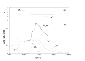
FIG. 8.: (a) Maslov index and (b) coherent superposition (“$2t_{0}+s^{\prime}$”,solid line with dots, ) of the $2t_{0}$ and $s^{\prime}$ contributions. We also show the contribution of the non self-retracing $s_{*}$ PO, and the QM results. (c) Experimental (line with crosses) and semiclassical (solid line) voltage periods.

The coherent superposition [$2t_{0}+s^{\prime}$] is much larger than the quantum amplitudes, because the individual isolated contributions are already as high as the QM results. Note the discontinuous change at $\epsilon=13600$; it is due to the discontinuous change of $\mu$ for $s^{\prime}$ at the pitchfork bifurcation. It is clear that the coherent superposition of $2t_{0}$ and $s^{\prime}$ cannot, whatever their relative phases, describe accurately the quantum results. Note that these POs are not involved together in a bifurcation; this is not the usual breakdown of semiclassics near a bifurcation, that one could solve with the use of normal forms (cubic expansions of the action). Also, $2t_{0}$ and $s^{\prime}$ seem to be well separated in position space (their starting positions are $z_{0}\simeq 0$ for $s^{\prime}$ and $z_{0}\simeq 600$ for $2t_{0}$).

Looking at quantum states contributing to the current reveals that the two POs are, in some sense, not isolated. A Wigner distribution and the related wave function are shown in Fig. 9.

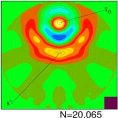
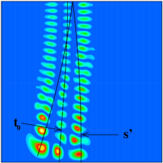
FIG. 9.: Left: Wigner distribution (color plot) at $\theta=27^{\circ},\epsilon=16000$ and classical Poincaré surface of section (dots), in the $(-p_{z},z)$ plane on the emitter wall. The square on lower-right corner represents $\hbar$. Right: corresponding wave function in the $(-z,x)$ plane, with the POs $t_{0}$ and $s^{\prime}$. The scales are the same as in Fig. 6.

The Wigner distribution has the familiar ring structure of a $k=2$ quantized torus in the stable island surrounding $t_{0}$. The ring is nevertheless distorted in some way and is also localized on the (here stable) PO $s^{\prime}$. Similarly, both POs are within the region of the localization of the wave function in position space. We can conclude that the quantum state cannot “distinguish” the two POs, and that the POs are hence non-isolated: they contribute collectively to the quantum state and to the current. The use of either SO or MO orbits, however, circumvents this problem and yields good results throughout.

E Comparison at $\theta=20^{\circ}$: divergence of the saddle orbit formula

Fig. 10 presents amplitudes for the period-two signal at $\theta=20^{\circ}$. The situation is similar to $\theta=27^{\circ}$; we do not present here the CCO formula. The low $\epsilon$ quantum peak can be described rather well by the PO (a), SO (b) or MO (c) formulae.

The quantum model can describe qualitatively the shape of the experimental peak at high $\epsilon$ (c), over a large range of parameters ($10000<\epsilon<40000$). The $15\%$ discrepancy is probably due to a small inaccuracy in the estimate of the decoherence time $\tau$. Semiclassically, we have the same two competing orbits as at $\theta=27^{\circ}$. Although its contribution is important, it seems that $s^{\prime}$ does not influence the quantum amplitudes. Note the difference between the $s^{\prime}$ contribution given by the PO/NO formula from the one given by the SO and MO formulae.

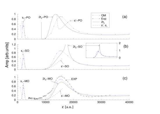
FIG. 10.: The different semiclassical theories for P2 amplitudes at $\theta=20^{\circ}$. The broad maximum is related to $2t_{0}$ and $s^{\prime}$ orbits, while the lower maximum is given by $s_{1}$ orbits. We show QM results and experimental readings [EXP]. (a) PO/NO formula. (b) SO formula. The inset is in a larger scale. (c) MO formula and experimental results.

The contribution of $2t_{0}$ to the PO/NO formula is good, but the position of the peak is not very accurate. The SO formula yields unexpected results: it has a very large peak (see inset), which we shall investigate below. The MO formula gives the correct position for the peak, but the height is not as precise as could be expected.

We investigate in Fig. 11 the large spike of the amplitude of the contribution of $2t_{0}\!-\!\!SO$ to the saddle orbit formula. We see in (a) that the reason for this is the fact that the determinant $\cal D$ [eq. (26)] of the quadratic expansion used in the SPA integration almost vanishes around $\epsilon=17500-17800$. Both its real (solid line) and imaginary (dashed line) part simultaneously approach zero. This is a remarkable coincidence, as $\cal D$ is a complex function, that one expects to vanish only if one can vary a parameter in the complex plane (i.e., two real parameters). In this case, varying $\epsilon$ only on the real axis approaches very closely the zero of $\cal D$, which should be reached for a value of $\epsilon$ with a small imaginary component.

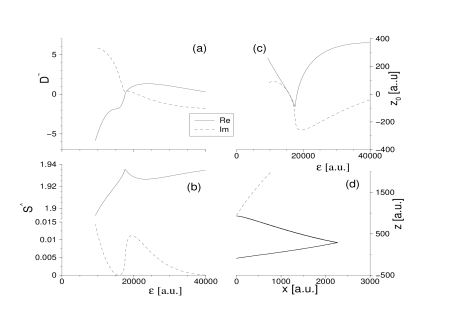
FIG. 11.: Classical characteristics of the SO $2t_{0}$ around the spike at $\epsilon\sim 17000-18000,\theta=20^{\circ}$. The solid line indicates the real component and the dashed line indicates the imaginary component. (a) Scaled determinant $\tilde{\cal D}={\cal D}/B$ [eq. (26)] of the quadratic expansion used in the SPA integration. (b) Scaled action $\hat{S}$. (c) Starting position $z_{0}$. (d) Real shape $({\rm I}{\rm Re}\>x,{\rm I}{\rm Re}\>z)$ of $2t_{0}\!-\!\!SO$ at $\epsilon=17476$; for fig. (d) the dashed line indicates the limit of the region allowed by (real dynamics) energy conservation.

The classical characteristics of $2t_{0}\!-\!\!SO$ in that region are not smooth. The real part of the action (b) reaches a maximum value at $\epsilon=17588$, while the imaginary part changes abruptly over the range $17000<\epsilon<18000$. The imaginary part of the starting position (c) behaves similarly. The real part of the starting position reaches the minimum value ${\rm I}{\rm Re}\>z_{0}=-89\>{\rm a.u.}$ at $\epsilon=17476$.

We show in (d) the real shape of $2t_{0}\!-\!\!SO$ at $\epsilon=17476$. The outer leg (with high ${\rm I}{\rm Re}\>z$) hits the left wall perpendicularly at a point which is very close (less than $20\>{\rm a.u.}$) to the limit surface of the region accessible by trajectories defined by real dynamics. This limit is where some self-retracing trajectories (like $s^{\prime}$ and $s_{1}$) have a turning point (i.e., have zero momentum). It is impossible to find trajectories with the same bounce structure ($2\!\!:\!\!2$) for ${\rm I}{\rm Re}\>z_{0}<-100$, because they would miss the intermediate bounce and go back to the right wall via the limit surface. This is similar to the “cusp bifurcation” of the PO $s^{\prime}$; it is also the only observed mechanism that can remove an SO, MO or CCO as $\epsilon$ changes.

As $\epsilon$ increases, ${\rm I}{\rm Re}\>z_{0}$ decreases until it reaches $-89\>{\rm a.u.}$. If it evolved smoothly, one would expect the SO at higher $\epsilon$ to start with a lower ${\rm I}{\rm Re}\>z_{0}$ –which seems impossible as we have seen that such starting condition did not allow the correct bounce structure. Hence, one would expect “a cusp disappearance” of $2t_{0}\!-\!\!SO$. This nevertheless does not happen: one can still find the SO for higher $\epsilon$, as abruptly increasing ${\rm I}{\rm Re}\>z_{0}$ satisfies the SO condition. Hence, it seems that we have a “failed” cusp disappearance of $2t_{0}\!-\!\!SO$, precisely in the region where the quadratic expansion becomes almost degenerate and where the classical characteristics of the orbit are not smooth.

This is altogether reminiscent of a bifurcation of periodic orbits, where two POs coalesce as the dynamical parameter ($\epsilon$) is varied, and where the quadratic expansion of the action (used e.g. in the GTF) becomes degenerate. However, PO bifurcations always involve more than one POs, while in this case we have not observed any neighboring SO that could coalesce with $2t_{0}\!-\!\!SO$.

Note that, strictly, one should not integrate (15) on the whole $(z,z^{\prime})$ plane, but only on the domain $\Omega$ where one does find the proper type of trajectories ($2\!\!:\!\!2$). Hence one should cut the integral for $z<-100$; this would yield Error functions.

This situation raises very interesting questions about saddle orbits. Do they undergo a type of bifurcation? Apparently no, as a bifurcation should involve several SOs, which we have not seen. What is the origin the quasi-degeneracy? It comes from a failed cusp disappearance. Does it has an effect on the semiclassical current? Yes, the current shows a strong enhancement. Do quantum results show any sign of it? Apparently no, as the QM results are smooth in that region. What techniques can be employed to solve that problem? We tried a cubic expansion of the action, which removed most of the enhancement but did not show good agreement with quantum calculations. One could try a cut-off in the integral. The first task would be to locate the complex value of $\epsilon$ for which ${\cal D}=0$.

V Conclusion

The general semiclassical formula (25) that we have developed summarizes in a compact way all the theories that have been proposed for the current in the RTD (excluding the changes required by the inclusion of excited Landau states and a shift of the Gaussian [10, 15]). It also shows clearly how the different assumptions on the smoothness of the Gaussian affect which type of orbits contribute to the current. We found the types giving the best semiclassical description: the complex saddle orbits (SOs) and the real minimal orbits (MOs). It appears that the more standard periodic or closed orbits do not succeed in all the situations, in particular in the ghost regions and where one has non-isolated contributions.

The (near) divergence of the saddle orbit formula at $\theta=0^{\circ}$ raises interesting questions about the SOs, namely the existence of a bifurcation-type phenomenon for trajectories defined by a pair of condition (33) as restrictive as the one defining POs (i.e., giving a discrete number of orbits). The complex dynamics we implemented here are very strongly restricted by the definition of the hard bounces on the barriers. One could obviously avoid this point by modeling the barriers by soft exponential walls. A preliminary study shows that the “cusp” bifurcations are replaced by standard tangent bifurcations; however the search for complex POs and SOs with soft barriers appears to be more difficult and again raises interesting questions about the high-dimensional search for complex POs and SOs.

The techniques used in this work could easily be applied to other systems involving Gaussian matrix elements, in particular Franck-Condon transitions and the conductance of microcavities with parabolic leads (where one further assumes that the lowest sub-band is occupied [14]). The importance of saddle or minimal orbits would then depend on the localization scale of the Gaussian.

The authors would like to thank E Bogomolny and D Rouben for invaluable help with the semiclassics and the complex dynamics, E Narimanov for communication of results prior to publication, and G Boebinger for unpublished experimental data. T S M acknowledges financial support from the EPSRC. D S S was supported by a TMR scholarship from the Swiss National Science Foundation.

A Phase-space semiclassics

Here we describe briefly a semiclassical formalism in phase space, similar to the one used in [7] and [10]. It is of course analytically equivalent to the position space formalism described in section II. We write $\bar{A}(\bar{z},\Delta z)$ (44) as the inverse Fourier transform

$$\bar{A}(\bar{z},\Delta z)=\int d\bar{p}W(\bar{z},\bar{p})e^{-i\bar{p}\Delta z/\hbar}$$ (A1)

of the Wigner function (45). We wrote $p\equiv p_{z}$ for convenience of notations. The integral (18) reads then

$${\cal I}=\sum_{\ell}\int d\bar{z}\int d\bar{p}\int d\Delta z\sqrt{\frac{p_{x}p^{\prime}_{x}}{-m_{12}}}W(\bar{z},\bar{p})e^{i\bar{\cal S}_{2}(\bar{z},\Delta z)/\hbar-i\bar{p}\Delta z/\hbar}\quad\mbox{.}\quad$$ (A2)

First one can integrate over $\delta\Delta z$ by Gaussian quadratures without any stationary approximation, which gives

$${\cal I}=\sum_{\ell}\int d\bar{z}\int d\bar{p}\sqrt{\frac{p_{x}p^{\prime}_{x}}{-m_{12}D}}W(\bar{z},\bar{p})e^{i[S_{0}+g(\bar{y},\bar{p})]/\hbar}$$ (A3)

with

$$g(\bar{z},\bar{p}) = -\bar{p}\Delta z_{0}+\delta\bar{z}\Delta p^{0}+\delta\bar{z}^{2}\frac{{\rm Tr}M-2}{2m_{12}}-2\left(\bar{p}^{0}-\bar{p}+\delta\bar{z}\frac{m_{22}-m_{11}}{2m_{12}}\right)^{2}\frac{m_{12}}{{\rm Tr}M+2}$$ (A4)

$$= \left[({\rm Tr}M+2)(-\bar{p}\Delta z_{0}+\Delta p^{0}\delta\bar{z})-2m_{12}\delta\bar{p}^{2}+2\delta\bar{p}\delta\bar{z}(m_{22}-m{{}_{11}})+2\delta\bar{z}^{2}m_{21}\right]/({\rm Tr}M+2)\quad\mbox{,}\quad$$ (A5)

$$D = \frac{{\rm Tr}M+2}{8m_{12}}$$ (A6)

where we have defined $\delta\bar{p}=\bar{p}-\bar{p}_{0}$. Integrating (A3) with the Gaussian Wigner transform (45) yields the same result as the integration in position configuration (25). The phase space formalism might be useful for stationary phase consideration, e.g. if one supposes that $W$ is smooth. Neglecting $W$ in the SPA condition applied to eq. (A3), one find periodic orbits, and integrating one find the result (51).

B COMPLEX DYNAMICS

This appendix presents a discussion of general aspects of complex dynamics in the RTD, which is based on empirical observations. It raises interesting questions, such as the definition of hard bounces in complex dynamics, the freedom in the evolution, and singularities.

We complexify the position $q$, the momentum $p$ and the time $t$. We keep the energy $E$ real, as it is a physical parameter given by the “reality” of the experiments ($E=RV$). As we know explicitly the formulae giving the evolution $\mbox{\boldmath$q$}(t),\mbox{\boldmath$p$}(t)$ between two bounces, we simply consider their analytical continuation is the complex plane. Computationally, we declare these variables as complex and evolve them following a given complex path for the time.

We illustrate the choice of the complex time path in Fig. 12. We start on the left barrier with ${\rm I}{\rm Re}\>x=0,{\rm I}{\rm Im}\>x=0$ and some complex initial condition $z_{0},p_{z}^{0}\in{\rm I}{\rm C}$. We evolve the time along the real axis $0<t<t_{b}$ until ${\rm I}{\rm Re}\>x(t_{b})=L$. For complex starting conditions, $x(t_{b})=L+iq_{b}$ is complex. Then we search for the complex time $T_{c}$ such that the imaginary part of $x$ becomes also zero [${\rm I}{\rm Im}\>x(T_{c})=0$]. This is done with a Newton-Raphson algorithm starting at $t_{0}=t_{b}$:

$$t_{n+1}=t_{n}-m\frac{x(t_{n})-L}{p_{x}(t_{n})}\quad\mbox{,}\quad T_{c}=\lim_{n\to\infty}t_{n}.\quad\mbox{.}\quad$$ (B1)

We consider that this situation defines a bounce on the right barrier, so we flip the $x$ momentum:

$${\rm bounce:}\quad\left\{\begin{array}[]{ll}{\rm I}{\rm Re}\>x(T_{c})=L\\ {\rm I}{\rm Im}\>x(T_{c})=0\end{array}\right.\quad\Rightarrow\quad\left\{\begin{array}[]{ll}{\rm I}{\rm Re}\>p_{x}\to-{\rm I}{\rm Re}\>p_{x}\\ {\rm I}{\rm Im}\>p_{x}\to-{\rm I}{\rm Im}\>p_{x}\quad\mbox{.}\end{array}\right.$$ (B2)

A bounce on the left barrier is obtained the same way, replacing $L$ by $0$ above. Then, we evolve again keeping ${\rm I}{\rm Im}\>t={\rm I}{\rm Im}\>T_{c}$, until one finds another barrier; we find the new complex time for which the bounce is “real”, flip the momentum and carry on.

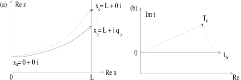
FIG. 12.: Scheme of the complex classical dynamics. (a) Real shape of a trajectory in the $({\rm I}{\rm Re}\>x,{\rm I}{\rm Re}\>z)$ plane. (b) Time path in the complex plane $({\rm I}{\rm Re}\>t,{\rm I}{\rm Im}\>t)$. The dashed lines correspond to the direct time path that goes to the bounce in a straight line. The dotted lines represent the Newton-Raphson algorithm (B1).

Note that although ${\rm I}{\rm Re}\>x$ decreases just before the bounce ($t<T_{c}$), ${\rm I}{\rm Re}\>p_{x}>0$ because ${\rm I}{\rm Re}\>t$ decreases as well. It is important here to emphasize the fact that the trajectory beyond the barrier is only a representation of the Newton-Raphson algorithm (B1), and does not represent any physical behavior. We have never defined what the potential is beyond the barrier; hence the particle does not feel any barrier until it reaches the time $T_{c}$. This is entirely different from the possibility that a particle has to tunnel through a finite height barrier, when it follows an imaginary time path or has complex momentum.

In real dynamics, the functions $\mbox{\boldmath$q$}(t),\mbox{\boldmath$p$}(t)$ between the bounces are analytical, with no discontinuity, divergence, singularity or apparent restriction. Their continuation in the complex plane is therefore holomorphic and single valued: $\mbox{\boldmath$q$}(t),\mbox{\boldmath$p$}(t)$ is uniquely defined, and does not depend on the specific path one has used to reach the time $t$. Using Cauchy’s theorem, one can deform a complex integral along an open path (keeping the starting and final points constant), provided one does not meet a pole of the integrated function. Hence, one can choose a “direct” time path which goes straight from $t=0$ to $t=T_{c}$ (see Fig. 12). The particle will arrive on the barrier directly with ${\rm I}{\rm Im}\>x(T_{c})=0$, and will undergo the bounce without venturing “beyond the barrier”. There is clearly an ambiguity related to the freedom of choosing a time path: each different time path yields a different looking trajectory [see Fig. 12(a)]. However, they all have the same global properties such as the total time $T$, action $S$, stability matrix $M$, final position and momentum as a consequence of the “analyticity” of the dynamics. As the current formulae or the Gutzwiller trace formula (GTF) use only the global properties of a certain type of trajectories, one can employ any convenient time path with reasonable safety. Other topics like the study of scarring (the localization of a quantum state on a trajectory) depend strongly on the shape of the trajectory, and are therefore more problematic to address. We always plot the “direct” time paths; they give trajectories that avoid the region beyond the barrier and are more similar to the trajectories found in real dynamics. For instance, a complex orbit looks self-retracing when the corresponding real orbit is self-retracing.

It is our definition of a bounce (B2), and the specification of the number of left and right bounces (the “bounce structure”) that determine uniquely the global structure of the time path in the complex plane. It has to go through the times $T_{c}^{i},i=1,2,..$ corresponding to each desired bounce. One could wonder if some points in the complex plane correspond to some sort of singularity in position or time (by singularity we mean either a pole or a point where the derivative is not defined.) In this case one should not deform the time path beyond this singular time, as this would yield a totally different trajectory. For example, Takada et al.[23] have related singularities to tunneling across a finite height potential barrier. So far, we never came across such singular points. Once again, we emphasize the fact that we do not have a finite height barrier, but define the infinite barrier through the condition (B2). Takada et al.[23] deformed the time path along the real axis ($-\infty<t<+\infty$) into the complex plane; pushing the deformation beyond a singular time corresponded to a tunneling event. Hence, going around a singular time changed the structure of the trajectory. Our approach here is different: we start at $t=0$ and must pass through the bounce times $T_{c}^{i}$. In a sense, the latter times are “singular” as the momentum changes there discontinuously; however they are not a discontinuity in the potential, one cannot go “around” them and there is no apparent barrier to tunnel into.

In the complex plane, multi-valued functions are behind the singular points where no derivative can be defined; they are the points where the different branches or Riemann sheets join. Semiclassical theories involve specific trajectories $(x=0,z)\to(x^{\prime}=0,z^{\prime})$, which can be “multi-valued”, in the sense that several starting momenta giving several different trajectories can nevertheless connect the same $z$ and $z^{\prime}$. In this case, the related singular point is a focal point where $m_{12}=0$; they appear in the $({\rm I}{\rm Re}\>z,{\rm I}{\rm Im}\>z;{\rm I}{\rm Re}\>z^{\prime},{\rm I}{\rm Im}\>z^{\prime})$ plane of starting and ending positions. We observed such singularities in contour plots of the action of TS orbits in the starting $z=z^{\prime}$ plane. As one goes around a complex focal point, one connects the different families of closed trajectories and one has a multi-valued action. They are entirely different from the hypothetical singularities in the time plane mentioned above.

It seems that this implementation of the complex dynamics restrict greatly the freedom that they usually offer. For instance, we cannot change the bounce structure of a complex orbit by changing the time path defining the evolution. A complex trajectory corresponding to a real trajectory having a turning point behaves also as if it has some kind of turning point (it turns back to the right wall without hitting the left wall); one cannot avoid this fact by trying to “force” a bounce on the left wall.

REFERENCES

- [1] M C Gutzwiller, Chaos in classical and quantum mechanics,New-York: Springer-Verlag (1990); see also M Brack and R K Bhaduri, Semiclassical physics, Reading, Mass.: Addison-Wesley (1997).
- [2] A Holle, J Main, G Wiebusch, H Rottke and K H Welge, Phys. Rev. Lett. 61, 161 (1988).
- [3] R Schinke and V Engel, J. Chem. Phys. 93, 3252 (1990).
- [4] H U Baranger, R A Jalabert and A D Stone, CHAOS 3, 665 (1993).
- [5] T M Fromhold, L Eaves, F W Sheard, M L Leadbeater, T J Foster and P C Main, Phys. Rev. Lett. 72, 2608 (1994).
- [6] G Müller, G S Boebinger, H Mathur, L N Pfeiffer and K W West, Phys. Rev. Lett. 75, 2875 (1995).
- [7] M Wilkinson, J. Phys. A 20, 2415 (1987): B Eckhardt, S Fishman, K Müller and D Wintgen, Phys. Rev. A 45, 3531 (1992).
- [8] M L Du and J B Delos, Phys. Rev. A 38, 1896 and 1913 (1988).
- [9] E B Bogomolny and D C Rouben, Europhys. Lett. 43, 111 (1998); Eur. Phys. J. B 9, 695 (1999).
- [10] E E Narimanov, A D Stone and G S Boebinger, Phys. Rev. Lett. 80, 4024 (1998).
- [11] E E Narimanov and A D Stone, Physica D 131, 221 (1999).
- [12] D S Saraga and T S Monteiro, Phys. Rev. Lett. 81, 5796 (1998).
- [13] O Zobay and G Alber, J. Phys. B 26, L539 (1993).
- [14] E E Narimanov, N R Cerruti, H U Baranger and S Tomsovic, eprint cond-mat/9812165 (1998).
- [15] D S Saraga, PhD Thesis University College London (unpublished, 1999), available at www.tampa.phys.ucl.ac.uk/ daniel/thesis.html.
- [16] J Bardeen, Phys. Rev. Lett. 6, 57 (1961).
- [17] T S Monteiro, D Delande, A J Fisher and G S Boebinger, Phys. Rev. B 56, 3913 (1997).
- [18] E E Narimanov and A D Stone, Phys. Rev. B 57, 9807 (1998).
- [19] W Miller, J. Chem. Phys. 63, 996 (1975).
- [20] D S Saraga and T S Monteiro, Phys. Rev. E 57, 5252 (1998).
- [21] T S Monteiro and P A Dando, Phys. Rev. E 53, 3369 (1996).
- [22] D S Saraga, T S Monteiro and D C Rouben, Phys. Rev. E 58, R2701 (1998).
- [23] S Takada, P N Walker and M Wilkinson, Phys. Rev. A 52, 3546 (1995).