Density-dependent diffusion in the periodic Lorentz gas

Abstract

We study the deterministic diffusion coefficient of the two-dimensional periodic Lorentz gas as a function of the density of scatterers. Results obtained from computer simulations are compared to the analytical approximation of Machta and Zwanzig [Phys.Rev.Lett. 50, 1959 (1983)] showing that their argument is only correct in the limit of high densities. We discuss how the Machta-Zwanzig argument, which is based on treating diffusion as a Markovian hopping process on a lattice, can be corrected systematically by including microscopic correlations. We furthermore show that, on a fine scale, the diffusion coefficient is a non-trivial function of the density. We finally argue that, on a coarse scale and for lower densities, the diffusion coefficient exhibits a Boltzmann-like behavior, whereas for very high densities it crosses over to a regime which can be understood qualitatively by the Machta-Zwanzig approximation.
KEY WORDS: deterministic diffusion; periodic Lorentz gas; computer simulations; random walk; chaotic scattering; symbolic dynamics; Boltzmann approximation; density expansion of transport coefficients

PACS numbers: 05.40.-a,05.45.-a,05.60.-k,51.10.+y

I Introduction

One of the central themes in the theory of chaotic transport is the problem of deterministic diffusion. Over the past several years, deterministic diffusion coefficients have been computed for a variety of low-dimensional model systems. The most elementary ones are chains of one-dimensional maps [1, 2, 3, 4], which have been studied with cycle expansion methods[5, 6, 7, 8]. By applying techniques based on Markov partitions it has been found that the deterministic diffusion coefficient of a simple piecewise linear one-dimensional map is a fractal function of the control parameter [9, 10]. Long-range dynamical correlations in the microscopic chaotic scattering processes of the system are responsible for this surprising behavior [10, 11, 12]. More complicated models exhibiting deterministic diffusion are two-dimensional maps such as multi-Bakers [13, 14, 15, 16], cat maps [17], standard maps [18], and related models [19]. Also in these models the diffusion coefficients are fractal [16], or are highly nontrivial functions of a control parameter [17, 18, 19].

These simple maps share fundamental physical and mathematical properties of more complicated dynamical systems such as the periodic Lorentz gas [20]. For this model, the diffusion coefficient has been computed with different methods: in Refs. [21, 22, 23] it has been obtained via the Green-Kubo formula on the basis of computer simulations, in Refs. [24, 25] techniques of cycle and periodic orbit expansions have been applied, and in Refs. [26, 27] the diffusion coefficient has been obtained from escape rate methods as well as from the Hausdorff dimension of the fractal repeller of the Lorentz gas.

In this paper we focus on the behavior of the diffusion coefficient in the two-dimensional periodic Lorentz gas under variation of the density of scatterers. In Section II we introduce the model, briefly sketch the simple analytical approximation obtained by Machta and Zwanzig [21] and compare it to our numerical results obtained from computer simulations. In Section III we explain how the Machta-Zwanzig argument can be corrected systematically by taking microscopic correlations into account. In Section IV we compare our numerical diffusion coefficient to a simple Boltzmann approximation and argue that, on a coarse scale, there is a dynamical crossover for the diffusion coefficient as a function of the density. More detailed computer simulations show that the diffusion coefficient exhibits a non-trivial fine structure as a function of the density, as is discussed in Section V. In Section VI we summarize our results and relate them to analogous findings in one- and two-dimensional maps.

II Diffusion as a simple Markov process: Machta-Zwanzig approximation and numerical results

The periodic Lorentz gas is a standard model in the field of chaos and transport [20, 28, 29, 30]. It mimics classical diffusion in a crystal and is isomorphic to a periodic system of two hard disks per unit cell [31]. The geometry of the model is shown in Fig. 1: A point particle of mass $m$ moves with constant velocity $v$ in an array of circular hard scatterers of radius $R$ arranged on a triangular lattice. Upon collisions with the scatterers the particle is reflected elastically. In the following we use units for which $v=1$, $m=1$, and $R=1$. The lattice spacing of the disks is then $2+w$, where $w$ is the smallest inter disk distance. The gap size $w$ is geometrically related to the number density $n$ of the disks by

$$n=2/[\sqrt{3}(2+w)^{2}]\quad.$$ (1)

The gap size $w$, or the number density of the disks $n$, respectively, is the only control parameter and completely determines the dynamical properties of the system. At close packing, i.e., $w=0$, the moving particle is trapped in a single triangular region formed between three disks (see Fig. 1). For $0<w<w_{\infty}=4\sqrt{3}-2=0.3094$, the particle can move across the entire lattice, but it cannot move collision-free for an infinite time. For $w>w_{\infty}$ the particle can move arbitrarily far between two collisions. Here, $w_{\infty}$ denotes the gap size at which the particle first sees such an “infinite horizon”. Bunimovich and Sinai proved that for $0<w<w_{\infty}$ the system is ergodic, and that the diffusion coefficient exists, while it diverges for $w>w_{\infty}$ [32, 33].

In Ref. [21] Machta and Zwanzig have derived a simple analytical approximation for the diffusion coefficient $D$. The basic idea is that diffusion can be treated as a Markovian hopping process between the triangular trapping regions indicated in Fig. 1. For this purpose, they have calculated the average rate $\tau^{-1}$ at which a particle leaves such a trap. According to a simple phase space argument, this rate is determined by the fraction of phase space available for leaving the trap divided by the total phase space volume of the trap. Furthermore, for random walks on two-dimensional isotropic lattices the diffusion coefficient is $D=l^{2}/(4\tau)$, where $l=(2+w)/\sqrt{3}$ is the distance between the centers of the traps. This leads to the Machta-Zwanzig random walk approximation of the diffusion coefficient

$$D_{\rm MZ}=\frac{w(2+w)^{2}}{\pi[\sqrt{3}(2+w)^{2}-2\pi]}\quad.$$ (2)

This equation is shown as the dotted line in Fig. 2. Included in this figure are single data points for the diffusion coefficient obtained by various authors using different methods: The filled circles are numerical results of Ref. [21], the stars are from Ref. [22]. These data points have been obtained by employing the Green-Kubo formula, where $D$ is determined from an integral over the velocity autocorrelation function. The squares have been computed in Ref. [25] by periodic orbit expansions, the empty circles and triangles are from Ref. [27], where they have been computed by applying the escape rate formalism, and via the fractal dimension of the repeller of the Lorentz gas, respectively. The crosses connected with lines represent our new data which we have obtained from computer simulations by means of the Einstein formula

$$D=\lim_{t\to\infty}\frac{\langle\Delta r^{2}(t)\rangle}{4t}\quad,$$ (3)

where the brackets indicate an ensemble average after time $t$. We calculated $\langle\Delta r^{2}(t)\rangle$ by averaging over long trajectories. Depending on the density $n$ each trajectory contained from $6\times 10^{8}$ to $3\times 10^{9}$ collisions. After a short transient $\langle\Delta r^{2}(t)\rangle$ grows linearly with a slope of $4D$. We determined the diffusion coefficient $D$ by fitting a straight line to $\langle\Delta r^{2}(t)\rangle$ in the linear regime. Though in principle equivalent with the Green-Kubo formalism, the Einstein approach is numerically more efficient in the Lorentz gas, where the equations of motion can be integrated exactly.

Fig. 2 shows that the Machta-Zwanzig approximation Eq. (2) is only correct in the limit of small gap sizes $w\to 0$. For larger values of $w$ and up to approximately $w<0.1$ Eq. (2) clearly overestimates the exact diffusion coefficient, whereas for $w>0.1$ it significantly underestimates diffusion. In the following section, we will discuss the physical reason for this failure of the Machta-Zwanzig approximation and how it can be corrected. Note also that for $w\to w_{\infty}$ there is no evidence for any singularity in the diffusion coefficient reminiscent of critical behavior. In Ref. [23], the same observation has been made based on the analysis of velocity autocorrelation functions. For explaining this lack of criticality the authors have argued that this transition rather represents a simple geometric feature of the system than being a consequence of long-range correlations.

III Correction of the Machta-Zwanzig approximation: correlated microscopic scattering

A Collisionless flights across a trap

As Machta and Zwanzig remarked themselves, for larger $w$ there is a non-vanishing probability $p_{\rm cf}$ for the particle to move collision-free across a trap. In Fig. 3 (a), we have calculated this probability from computer simulations as well as in a straightforward analytical approximation, which is described in Appendix A. Note that collisionless flights occur only for $w>0.1547$, see Eq. (A6).

If we rely on the Machta-Zwanzig picture of diffusion as a hopping process with frequency $\tau^{-1}$ over distances $l$, we can correct Eq. (2) in the following way: If a particle moves collision-free across a trap, it travels within the time $\tau$ over a larger distance than assumed in Eq. (2). For this larger distance we take the distance between a center of a trap and the center of its next nearest neighbor which is $l_{2}=\sqrt{3}l$. These processes would thus yield a larger diffusion coefficient $D_{l_{2}}=l_{2}^{2}/(4\tau)=3D_{MZ}$, where $D_{MZ}$ is the diffusion coefficient of Eq. (2). We now define the corrected Machta-Zwanzig diffusion coefficient $D_{\rm cf}$ by weighting the contribution of collisionless flights via the probability $p_{\rm cf}$ of Fig. 3 (a),

$$D_{\rm cf} = [1-p_{\rm cf}]D_{MZ}+p_{\rm cf}3D_{MZ}$$ (4)

$$= [1+2p_{\rm cf}]D_{MZ}\quad.$$ (5)

The result is plotted in Fig. 3 (b). For $w>0.1547$, the revised formula Eq. (5) improves the original Machta-Zwanzig approximation considerably, however, it is still much smaller than the numerically exact results.

B Probability of backscattering

A second significant contribution to the correction of Eq. (2) is determined by the backscattering probability $p_{\rm bs}$, which is the probability of the moving particle to leave the trap through the same gap where it entered. We computed $p_{\rm bs}$ numerically by repeatedly injecting the particle through a specific gap and observing trough which gap it left the trap. The particles are initially situated at one entrance of a trap, and they are uniformly distributed in the respective phase space of this entrance, which consists of the position of a particle on the entrance line, $-1\geq 2x/w\geq 1$, and of the sine of the angle between the velocity direction and an axis perpendicular to the entrance, $-1\geq\sin\alpha\geq 1$. Alternatively, $p_{\rm bs}$ can be determined from a single long trajectory. The backscattering probability obtained from our simulations is shown in Fig. 4 (a).

The Markovian approximation of Machta and Zwanzig Eq. (2) corresponds to a backscattering probability of $1/3$. However, for small values of $w$ the numerically computed probability is significantly larger than $1/3$, whereas for larger $w$ it is considerably smaller. The reduced probability for backward scattering at larger $w$ is in part due to collisionless flights across the trap. It is remarkable that the backscattering probability is different from $1/3$ even for gap sizes where the average number of collisions between inter-trap hops is large. At $w=0.055$, where the backscattering probability reaches its maximum value of $p_{\rm bs}=0.38$, more than 17 collisions occur before the particle hops to the next trap and for $w=0.02$, where $p_{\rm bs}$ is still close to $0.36$, the number of collisions is greater than $50$. Correspondingly, the detailed functional form of $p_{\rm bs}$ appears to be quite intricate: Below the maximum at $w=0.055$ there are at least three regions where $p_{\rm bs}$ decreases approximately linear in $w$ with different values of the slope. As the numerical results indicate, the function must eventually drop extremely sharply to $p_{\rm bs}(0)=1/3$. Details of these regions are shown in the magnification included in the figure. The vertical lines separating different regions correspond to the respective lines separating regions of different slope in the main figure. A very close look reveals that the fine structure of all these different regions appears to be quite similar, however, we note that this structure is essentially within the range of our numerical errors.

Fig. 5 shows the initial conditions in the $(x,\sin\alpha)$-plane leading to backscattering for a gap size of $w=0.1$. Here, the $x$-axis is parallel to the trap entrance and the origin is located at the center of the entrance. Initial conditions were drawn at random from a uniform distribution in this plane and a dot was plotted whenever the particle left the trap through the same aperture where it entered. Simulations at different densities yield similar pictures. The complicated, intertwined structure is reminiscent of a fractal set. The modifications of this structure by varying $w$ must be related to the changes seen in the function $p_{\rm bs}$ of Fig. 4 (a). This may explain why, even on the coarse scale of 4 (a), $p_{\rm bs}$ is not a simple function of $w$. Moreover, the detailed changes of this fractal set may be reflected in the respective detailed changes of $p_{\rm bs}$ on the fine scale, as illustrated in the magnification.

Having the probability of backscattering $p_{\rm bs}$ we can now perform a second correction of the original Machta-Zwanzig diffusion coefficient Eq. (2). For this purpose, we again assume that diffusion can be treated as a hopping process with a frequency $\tau^{-1}$ over distances $l$. We now inquire to which traps the particle can move by performing two jumps within a total time interval of $2\tau$. There are only two possibilities: either the particle suffers backscattering, that is, it goes back to its original trap and does not contribute to any actual displacement within $2\tau$, or it moves over a distance $l_{2}$ to the left or to the right of its original trap. Thus, the corresponding diffusion coefficient reads

$$D_{\rm bs} = \frac{[1-p_{\rm bs}]l_{2}^{2}}{8\tau}$$ (6)

$$= [1-p_{\rm bs}]3/2D_{MZ}\quad.$$ (7)

$D_{\rm bs}$ is plotted in comparison to our Einstein formula results, and to the original Machta-Zwanzig Eq. (2), in Fig. 4 (b). For smaller $w$, the corrected diffusion coefficient approximates the numerically exact values quite well. Thus, we conclude that the existence of backscattering is basically responsible for the Machta-Zwanzig argument overestimating diffusion for small values of $w$. For larger $w$ Eq. (7) again improves the original Machta-Zwanzig approximation, like the previous approximation Eq. (5), however, like this it yields much smaller results than the correct values.

C Combining collisionless flights, backscattering, and a symbolic dynamics

So far we have identified two different microscopic scattering mechanisms which were not included in the original Machta-Zwanzig approximation for the diffusion coefficient, and which evidently play a significant role for understanding the full density-dependent diffusion coefficient: Namely, the probability of collisionless flights across a trap leading to the diffusion coefficient of Eq. (5), and the probability of backscattering leading to Eq. (7). Consequently, one may think of combining these two different approximations within a single diffusion coefficient formula. This can be performed by simply replacing the Machta-Zwanzig diffusion coefficient $D_{MZ}$ in Eq. (7) by $D_{\rm cf}$ of Eq. (5) yielding

$$D_{1}=3/2[1-p_{\rm bs}][1+2p_{\rm cf}]D_{MZ}\quad.$$ (8)

This function, denoted as a first order approximation, is shown in Fig. 6 (a) in comparison to the numerically exact results and to the Machta-Zwanzig Eq. (2). For larger $w$, this combined approximation is much closer to the numerical results than the original Machta-Zwanzig formulation, however, there still remains a notable quantitative difference.

In the same figure, corrections of higher order based on the idea of Eq. (8) are depicted. In the following we just outline the basic concept, the detailed formulas are then given in Appendix B. The higher-order corrections of the diffusion coefficient are obtained by numerically computing the probabilities of higher-order backscattering, and by building them into a respectively generalized version of Eq. (7). This generalized expression of the backscattering diffusion coefficient $D_{\rm bs}$ is then combined with the respective collisionless flight-diffusion coefficient $D_{\rm cf}$ of Eq. (5) in the same way as before. The probabilities of higher-order backscattering have been computed on the basis of a simple symbolic dynamics, as it can be defined in case of simple backscattering: We followed a long trajectory of a particle in the Lorentz gas. For each visited trap we labeled the entrances through which the particle entered with $z$, the exit to the left of this entrance with $l$, and the one to the right with $r$. Thus, a trajectory in the Lorentz gas can be mapped to a sequence of symbols $z,l$, and $r$. Note that the symbolic dynamics we are using here is different to the one applied in other work in that we are labeling the three gaps of a trap, whereas in previous work the single disks accessible after a collision have been chosen, which required an alphabet of 12 symbols [8, 20]. $p(z)=p_{\rm bs}$ is then the backscattering probability depicted in Fig. 4 (a), whereas, due to symmetry, $p(l)=p(r)=(1-p(z))/2$ corresponds to forward scattering. Combining these probabilities with the correction by collisionless flights yields Eq. (8) as a first order approximation.

Higher-order correlations can be calculated by taking into account the probabilities of longer symbol sequences. For example, the second order approximation involves probabilities corresponding to nine symbol sequences each consisting of two symbols, $p(zz)$, $p(zl)$, $p(zr)$, $p(lz)$, $p(ll)$, $p(lr)$, $p(rz)$, $p(rl)$, $p(rr)$. In complete analogy to Eq. (8), a respective second-order approximation of the diffusion coefficient is then computed on the basis of these numerical probabilities, and by associating to them the respective distances traveled within a time interval of $3\tau$, see Eq. (B1). In the third-order approximation the probabilities correspond to sequences of three symbols, for example, three times backscattering within a time interval of $4\tau$ corresponding to $p(zzz)$, etc., and lead to the diffusion coefficient of Eq. (B2). In general, the $k$-th order approximation involves the probability of sequences of $k$ symbols. Fig.6 (a) shows that by including such correlations the respective higher-order approximations of the diffusion coefficient converge, and basically move closer to the numerical exact results. However, for $w>0.1$ the approximations converge to the exact results apparently only globally, and not locally. A clear sign of this is that in third order the respective approximation already exceeds the numerical data for large $w$, although the approximations seem to approach the exact data generically from below. On the other hand, one should take into account that this approximation scheme is based on a purely heuristical ansatz for the diffusion coefficient. Thus, an exact convergence should not necessarily be expected.

We therefore studied the effect of increased (or decreased) backscattering with the help of a lattice gas computer simulation. In such a simulation the Lorentz gas is mapped to a honeycomb lattice where the sites of the lattice represent the traps. The moving particle hops from site to site with frequency $\tau^{-1}$ , which is identical to the exact hopping frequency used in Machta-Zwanzig theory. We first describe the first order approximation: At each step the particle hops back to the site where it came from with probability $p_{\rm bs}$ or to one of the other sites with probability $(1-p_{\rm bs})/2$. The backscattering probability $p_{\rm bs}$ used in the lattice gas simulations is the one numerically obtained from simulations in the Lorentz gas. Also in the lattice gas simulations we determine the diffusion coefficient from the Einstein formula Eq. (3). The results of these simulations are shown in Fig. 6 (b) by a dotted line. Taking into account these first order correlations brings the diffusion coefficient closer to the correct value, but there still is a considerable deviation. This indicates the importance of higher order correlations.

These higher order correlations can be obtained by correlating more than two hops between neighboring traps. To determine the diffusion coefficient for such multiple hopping events by lattice gas simulations we used the probabilities $p(lrz)$ calculated up to fourth order from long trajectories in the Lorentz gas. The results of these calculations are shown in Fig. 6 (b). As can be seen in the figure, the diffusion coefficient obtained from this scheme converges very quickly to the numerically exact results, in particular for small $w$. For larger $w$, the convergence is somewhat slower, however, the fourth order approximation can be hardly distinguished from the numerically exact results on the scale of Fig. 6 (b). For growing order the diffusion coefficient converges to the correct results exactly.

IV Boltzmann approximation for the diffusion coefficient

In the previous section, we have discussed how the Machta-Zwanzig theory can be improved systematically. An alternative approach for understanding diffusion in the Lorentz gas may be obtained from kinetic theory, which essentially applies at low densities. In Refs. [34, 35], the Boltzmann approximation for the random Lorentz gas, where the scatterers are distributed randomly in the plane without overlap, has been used to compute the diffusion coefficient to

$$D_{\rm Bo}(n)=\frac{3}{8}l_{c}(n)v\quad,$$ (9)

where $l_{c}=1/(2Rn)$ is the collision length of the moving particle. At higher number densities $n$ the excluded volume of the scatterers becomes important, and the respective shorter collision length reads

$$D_{\rm Bo}(n)=\frac{3}{16}(\frac{1}{n}-\pi)\quad,$$ (10)

where we have changed to units with $v=1$ and $R=1$. The same result for the collision length can be obtained directly from the Machta-Zwanzig argument of Section II [21]. In case of the periodic Lorentz gas $n$ is related to the gap size $w$ by Eq. (1). Note that for $w=0$, where the particle is trapped, the corresponding density is $n<\infty$ and the collision length is still finite. Thus, Eq. (10) implies a diffusion coefficient of $D_{\rm Bo}(w=0)>0$, that is, this approximation inevitably leads to an offset between $D_{\rm Bo}(w=0)$ and the exact result of $D(w=0)=0$. Therefore, it can immediately be concluded that $D_{\rm Bo}$ is not correct at the highest densities.

In Fig. 7, Eq. (10) is shown in comparison to the numerically exact results and to the Machta-Zwanzig approximation Eq. (2). For this purpose, the diffusion coefficient has been plotted as a function of $1/n$, and an offset of $\Delta D=0.025$ has been subtracted from Eq. (10). According to this equation, $D_{\rm Bo}(n)$ should go linear in $1/n$ with a slope of $3/16$, and the offset $\Delta D$ is the only fit parameter. Indeed, Fig. 7 shows that, on a sufficiently coarse scale and over a wide range of lower densities, $D$ matches quite well to this functional form. In particular, the value of the slope appears to be almost exact. Only for larger densities $D$ deviates from linearity in $1/n$. However, here the Machta-Zwanzig approximation seems to describe the functional form at least qualitatively quite well.

From a conceptual point of view one may inquire why a Boltzmann description should at all be applicable to the periodic Lorentz gas. The basic difficulty is that because of the occurrence of an infinite horizon, a diffusion coefficient exists in the periodic Lorentz gas only in the regime of very high densities, where a simple Boltzmann approximation may not necessarily be expected to work. We first remark that in a Lorentz gas there are no density corrections due to screening of particles, or to many-particle collisions, as they are contained in an Enskog equation [36]. However, the existence of an offset at large densities may be related to the fact that the Boltzmann approximation represents only the first term in a series expansion in $n$, which is known as the density expansion of kinetic theory. For the random Lorentz gas, such a density expansion has been carried out explicitly in Refs. [34, 35]. It has been found that there exist higher-order terms being logarithmic in the density corresponding to so-called ring collisions, which diminish the Boltzmann diffusion coefficient quantitatively. However, these logarithmic corrections are difficult to see in the functional form of the diffusion coefficient. It is not known to us whether a density expansion has been performed for the periodic Lorentz gas. But the offset we find might be associated to the existence of such higher-order corrections in the density, and the apparent Boltzmann-like linear behavior may be related to the observation that in similar systems higher-order corrections do not change the functional form of the diffusion coefficient in a drastic way.

Because of the functional relation between number density $n$ and gap size $w$ Eq. (1), and according to the Boltzmann approximation Eq. (10), there should exist a respective approximate linear dependence of the diffusion coefficient $D$ on $w$, as can in fact be seen in Fig. 2. The quadratic term in $w$ which appears in Eq. (1) turns out to be quantitatively at most $6\%$ for largest $w$, and, after a proper adjustment, cannot be seen as any deviation to a linearity in $w$.

V Fine structure of the diffusion coefficient

To learn more about the very detailed dependence of $D$ on the density $n$, or alternatively on the gap size $w$, we performed further computer simulations in the region of large $w$. The results are shown in Fig. 8. Here, the respective residuals of $D$ have been plotted, that is, the deviation of the diffusion coefficients from a linear fit in $w$ over the whole region shown in the figure. At each value of $w$ ten independent runs of more than $2\times 10^{9}$ collisions each have been carried out yielding the diffusion coefficients shown by the dots. The squares correspond to the averages over the ten runs, where the size of the squares indicates the size of the numerical error. Fig. 8 may be regarded as a signature of long-range correlations in microscopic scattering events. A certain subclass of such scattering events are the ring collisions mentioned above leading to a series of logarithmic corrections, and divergences, in the density expansion of the diffusion coefficient. It might be conjectured that the existence of these divergences in the density expansion of kinetic theory is due to the problem of approximating a diffusion coefficient, which is in fact a function as complicated as the one shown in Fig. 8, in form of a simple series expansion, as has already been remarked in Ref. [20].

VI Conclusions

We have numerically computed the density dependence of the diffusion coefficient in the two-dimensional periodic Lorentz gas. A comparison of our results with the analytical approximation of Machta and Zwanzig shows that their argument is only asymptotically correct in the limit of high densities. We have furthermore discussed how their approximation can be corrected systematically by including correlations in the hopping mechanism.

As an alternative way to understand the structure of the density-dependent diffusion coefficient, we compared our numerical results to a simple Boltzmann approximation. We found that on a coarse scale there exists a dynamical crossover from a function linear in $1/n$ for lower densities, as qualitatively be described by the Boltzmann diffusion coefficient, to a behavior at high densities which can qualitatively be understood by the Machta-Zwanzig argument. Our two different points of view of understanding the density-dependent diffusion coefficient - namely, on the basis of the Machta-Zwanzig argument, and by a Boltzmann approximation -, are not at all contradictory. The complicated microscopic scattering processes responsible for the failure of the Machta-Zwanzig approximation apparently just superpose in a way such that the resulting diffusion coefficient is approximately linear in $1/n$ on a coarse scale. A similar relation between nonlinear corrections and a linear response has been discussed in Refs. [37, 38] with respect to the existence of Ohm’s law in a periodic Lorentz gas with an external field. That this picture is too simple is demonstrated by the fact that on a very fine scale we find deviations from such a simple linear behavior. These tiny fluctuations may be regarded as the signature of specific microscopic correlated scattering processes in the deterministic diffusion coefficient.

A dynamical crossover between different asymptotic laws for a parameter-dependent diffusion coefficient has already been found and discussed in related periodic one-dimensional chaotic maps [10, 11]. As in our discussion above, for these maps two different random walk models have been used to describe the corresponding asymptotic behavior: For small parameters, the respective random walk basically depends on the hopping probability of a particle leaving a cell, thus corresponding to the Machta-Zwanzig approximation, whereas for larger parameters the respective random walk scales with the distance a particle travels per time step, thus corresponding to the Boltzmann approximation, where diffusion is proportional to the collision length of the moving particle. We furthermore note that the diffusion coefficients in this kind of maps have been found to be fractal with respect to variation of the control parameter, and that specific correlated microscopic scattering events could be identified as being responsible for this fractal structure [9, 10]. The same phenomena have been encountered in related two-dimensional multi-baker maps, which are simple toy models of the periodic Lorentz gas [16].

Whether the density-dependent diffusion coefficient of the periodic Lorentz gas is in fact a non-differentiable function of the parameter, as it is the case for the one-dimensional maps discussed above, remains an open problem. It seems to us that this question cannot be answered by performing straightforward computer simulations, but that, instead, more refined techniques to compute the diffusion coefficient are necessary, as they have been developed, for example, in Ref. [10] in case of one-dimensional maps. A solution to this problem appears to be important for a complete understanding of deterministic diffusion in the periodic Lorentz gas.

Acknowledgments
This article is dedicated to G. Nicolis on occasion of his 60th birthday. R.K. wants to express his gratitude to G. Nicolis for many scientific discussions and advice, and for his continuing support over the last two years. In addition, R. K. is indebted to P. Gaspard for his interest in this problem, and for many valuable discussions. Helpful comments by E. Barkai, H. van Beijeren and D. Panja are gratefully acknowledged. Finally, R.K. thanks the European Commission for financial support within its Training and Mobility Program.

A Probability for a collisionless flight across a trap

In this part of the Appendix we describe a simple analytical approximation by which the probability $p_{\rm cf}$ for a collisionless flight across a trap can be computed. The result is shown in Fig. 3 (a). Our approximation is based on straightforward applying the Machta-Zwanzig phase space argument described in Section II. It says that

$$p_{\rm cf}=\frac{Sv\tau\phi}{2\pi A}\quad,$$ (A1)

where $A$ is the area of the trap, $2\pi$ is the measure of the velocity space of the trap, $S$ is the region of the boundary of the trap across which collisionless flights are possible, $v=1$ is the velocity of the moving particle, $\tau$ is the average time at which a particle leaves the trap, and

$$\phi=\int d\gamma\>\underline{n}\cdot\underline{v}\>\varrho(\gamma)$$ (A2)

is the average flux of particles with velocity $\underline{v}$ parallel to the normal $\underline{n}$ at one entrance, with $\gamma$ being the angle between $\underline{n}$ and $\underline{v}$, and $\varrho(\gamma)=\cos\gamma$ being the invariant probability distribution of $\gamma$ in equilibrium. Here we have already assumed that, in an approximation, $\phi$ is completely independent of its position at the boundary. In Ref. [21] it has been noted that

$$\tau=\frac{\pi A}{3w}\quad,$$ (A3)

where $w$ is the size of an entrance, such that Eq. (A1) reads

$$p_{\rm cf}=\frac{S\phi}{6w}\quad.$$ (A4)

Thus, it remains to compute $S$ and $\phi$. The relevant variables for this purpose, and the geometry, are defined in Fig. 9, where, because of symmetry, we have reduced the problem to one entrance. In a second approximation, we assume that regions of size $e$, as the one indicated in the figure, are the only parts of the boundary which contribute to free flights. $e$ is precisely defined as the section on the entrance line between the two horizontal lines which touch the upper scatterer tangentially, and which go from the lower edge of the left entrance to the lower edge of the right entrance, respectively. Because of symmetry, there are six regions like this for each trap leading to $S=6e$. $e$ can simply be calculated to

$$e=\frac{\sqrt{3}(2+w)}{2\sin(\pi/3)}-\frac{1}{\sin(\pi/3)}-1\quad.$$ (A5)

Note that only for $e>0$ collisionless flights across a trap are possible. In other words, $e=0$ or, by employing Eq. (A5),

$$w_{0}=\frac{2(\sin(\pi/3)+1)}{\sqrt{3}}-2\simeq 0.1547$$ (A6)

marks just the onset of the existence of collisionless flights with respect to varying $w$.

It now remains to compute the flux $\phi$ in these regions. To do this, we need to know the limits of the integral in Eq. (A2). As a very crude approximation, we assume that these boundaries are determined by the angles $\beta$ and $\delta$ such that

$$\phi = \int_{\beta-\delta}^{\beta+\delta}d\gamma\>\cos^{2}\gamma$$ (A7)

$$= \delta+1/2\cos(\pi/12)\sin(2\delta)\quad.$$ (A8)

Here, $\beta=\pi/6$ is identical to the angle between a horizontal velocity vector $\underline{v}$ and the normal $\underline{n}$ of the entrance. $\delta$ gives a bound for the directions the velocity $\underline{v}$ can take such that a particle going in through the region of size $e$ can perform a collisionless flight across the trap. By a straightforward calculation, it can be found that

$$\delta=\arctan\frac{2e\cos(\pi/6)}{2+w-2(e+1)\cos(\pi/3)+e\sin(\pi/6)}\quad.$$ (A9)

In summary, we have computed the probability $p_{\rm cf}$ for collisionless flights across a trap as

$$p_{\rm cf}=\frac{e\phi}{w}\quad,$$ (A10)

where $e$ is given by Eq. (A5), and $\phi$ is given by Eqs. (A8) and (A9).

B Higher-order backscattering approximations of the diffusion coefficient

Here we give the explicit formulas for higher-order approximations of the diffusion coefficient in the spirit of Eq. (8), where this equation represents already the first order correction. The basic idea of these corrections is discussed in Section III C.

The underlying picture for all these approximations is the Machta-Zwanzig assumption of diffusion as a hopping process with frequency $\tau^{-1}$ on a hexagonal lattice of traps, where the lattice sites are separated by a distance of $l$. We use in the following the symbolic dynamics introduced in Section III C to denote the transition probabilities of a particle which hops from one initial trap to some other trap on the lattice within a certain time interval of multiples of $\tau$. For the particular time interval of $3\tau$, we find that the particle can move

– with a probability $p_{1}=p(zz)+p(zl)+p(zr)+p(lz)+p(rz)$ over a distance $l_{1}=l=(2+w)\sqrt{3}$
– with a probability $p_{3}=p(lr)+p(rl)$ over a distance $l_{3}=\sqrt{7}l$
– with a probability $p_{3^{\prime}}=p(ll)+p(rr)$ over a distance $l_{3^{\prime}}=2l$.

The corresponding second-order diffusion coefficient then reads

$$D_{2}=(12\tau)^{-1}[p_{1}l_{1}^{2}+p_{3}l_{3}^{2}+p_{3^{\prime}}l_{3^{\prime}}^{2}]\quad.$$ (B1)

In the same way the third-order approximation is obtained. Here, we have a collection of 27 probabilities corresponding to the different lattice sites where the particle can move within a time interval of $4\tau$. These transition probabilities are labeled by all possible combinations of the three symbols l, r, and z corresponding to sequences of three symbols. Thus, the particle can move

– with a probability $p_{0}=p(lzz)+p(rzz)+p(zlz)+p(zrz)+p(zzz)$ over a distance $l_{0}=0$
– with a probability $p_{2}=p(lll)+p(llz)+p(lrz)+p(lzl)+p(lzr)+p(rlz)+p(rrr)+p(rrz)+p(rzl)+p(rzr)+p(zll)+p(zlr)+p(zrl)+p(zrr)+p(zzl)+p(zzr)$ over a distance $l_{2}=\sqrt{3}l$
– with a probability $p_{41}=p(lrl)+p(rlr)$ over a distance $l_{41}=3l$
– with a probability $p_{42}=p(llr)+pp(lrr)+p(rll)+p(rrl)$ over a distance $l_{42}=(1.5+\sqrt{3})l$.

The corresponding second-order diffusion coefficient then reads

$$D_{3}=(16\tau)^{-1}[p_{2}l_{2}^{2}+p_{41}l_{41}^{2}+p_{42}l_{42}^{2}]\quad.$$ (B2)

Eq. (B1) thus corresponds to the second-order approximation plotted in Fig. 6 (a), and Eq. (B2) yields the respective third-order approximation.

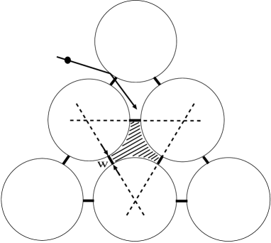
FIG. 1.: Geometry of the periodic Lorentz gas. A point particle scatters elastically at hard disks arranged on a triangular lattice. The cross-hatching indicates a single triangular trapping region. The smallest interdisk distance is denoted by $w$.

FIG. 2.: Diffusion coefficient $D$ as a function of the gap size $w$. The dashed line represents the Machta-Zwanzig random walk model Eq. (2), the different symbols refer to single data points obtained in the literature from various methods (see text). The crosses connected with lines are our new results from computer simulations. All of our data points have error bars smaller than the symbols. Error bars of the other data points have been included as far as available.

(a)                                          

(b)                                                

FIG. 3.: Correction of the Machta-Zwanzig approximation by collisionless flights: (a) probability $p_{\rm cf}$ of collisionless flights across a trap, numerical results (dotted line with crosses), and the analytical approximation Eq. (A10) (bold line) (b) diffusion coefficient $D$, numerical results (bold line with crosses) in comparison to the Machta-Zwanzig approximation Eq. (2) (dotted line), and compared to the correction of Eq. (5) by including $p_{\rm cf}$ (dashed line).

(a)                                       

(b)                                                

FIG. 4.: Correction of the Machta-Zwanzig approximation by backscattering: (a) backscattering probability $p_{\rm bs}$ as a function of the gap size $w$. For larger $w$ the single data points are plotted by symbols and are connected with lines, for smaller $w$ only the lines are shown. The dotted line corresponds to the value of $1/3$ of equal probability for any gap, as it is assumed in the Machta-Zwanzig approximation. The inset is a half-logarithmic blowup of the initial region for small $w$. The bars included in the figure refer approximately to the regions of different slope in the main figure. (b) numerical results for the diffusion coefficient (bold line with crosses) in comparison to the Machta-Zwanzig approximation Eq. (2) (dotted line), and to the correction via $p_{\rm bs}$ Eq. (5) (dashed line).

FIG. 5.: Initial conditions yielding backscattering for $w=0.1$. Each dot represents an initial condition for which the particle leaves the trap through the same aperture where it entered. $2x/w$ is the position of a particle on the line of the entrance, and $\alpha$ is the angle of flight of an in-going particle to an axis perpendicular to the entrance.

(a)                                                

(b)                                                

FIG. 6.: Systematic approximations of the exact diffusion coefficient in higher order: (a) combined approach of employing the numerical probabilities of collisionless flights and of backscattering within a hierarchy of analytical expressions of the diffusion coefficient. The first-order approximation is given by Eq. (8) by using the probabilities $p_{\rm cf}$ and $p_{\rm bs}$ of Figs. 3 (a) and 4 (a). The second order corresponds to Eq. (B1), and the third order corresponds to Eq. (B2). They include higher-order backscattering events, as described in the text and in Appendix B. (b) diffusion coefficients obtained from lattice gas simulation by using probabilities of correlated hopping sequences as calculated in Lorentz gas simulations (see text).

FIG. 7.: Diffusion coefficient in the periodic Lorentz gas with respect to the inverse of the number density of the scatterers $n$. The Boltzmann approximation Eq. (10) is shown after subtracting an offset of $\Delta D=0.025$ (thin bold line). It is compared to the numerically exact results (thick bold line with crosses), and to the Machta-Zwanzig approximation Eq. (2).

FIG. 8.: Residuals of $D)$, that is, the difference between the numerically computed diffusion coefficient $D$ and a linear fit over the range of the data presented in the figure. The dots indicate the results of ten independent runs for each value of $w$, the squares represent the algebraic averages over these ten runs. The size of the squares is equal to the magnitude of the numerical error.

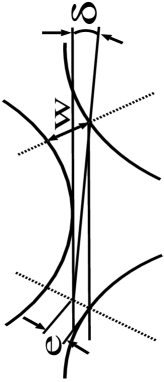
FIG. 9.: Geometry to compute the probability of collisionless flights $p_{\rm cf}$ across a trap. $e$ labels the size of one of the two regions at any of the three entrances of the trap where ingoing particles can perform collisionless flights. $\delta$ is related to an approximate bound for the directions the velocity of such a particle can take such that it performs a collisionless flight.

REFERENCES

- [1] H. Fujisaka and S. Grossmann, Z. Physik B 48, 261 (1982).
- [2] T. Geisel and J. Nierwetberg, Phys. Rev. Lett. 48, 7 (1982).
- [3] M. Schell, S. Fraser, and R. Kapral, Phys. Rev. A 26, 504 (1982).
- [4] E. Barkai and J. Klafter, Phys. Rev. Lett. 79, 2245 (1997).
- [5] R. Artuso, Phys. Lett. A 160, 528 (1991).
- [6] H.-C. Tseng et al., Phys. Lett. A 195, 74 (1994).
- [7] C.-C. Chen, Phys. Rev. E 51, 2815 (1995).
- [8] P. Cvitanović, lecture notes, available on www.nbi.dk/ChaosBook/ .
- [9] R. Klages and J.R. Dorfman, Phys. Rev. Lett. 74, 387 (1995).
- [10] R. Klages, Deterministic diffusion in one-dimensional chaotic dynamical systems (Wissenschaft & Technik-Verlag, Berlin, 1996).
- [11] R. Klages and J.R. Dorfman, Phys. Rev. E 55, R1247 (1997).
- [12] R. Klages and J.R. Dorfman, Phys. Rev. E 59, 5361 (1999).
- [13] P. Gaspard, J. Stat. Phys. 68, 673 (1992).
- [14] S. Tasaki and P. Gaspard, J. Stat. Phys. 81, 935 (1995).
- [15] J. Vollmer, T. Tél, and W. Breymann, Phys. Rev. Lett. 79, 2759 (1997).
- [16] P. Gaspard and R. Klages, Chaos 8, 409 (1998).
- [17] I. Dana, N. Murray, and I. Percival, Phys. Rev. Lett. 65, 1693 (1989).
- [18] A. Rechester and R. White, Phys. Rev. Lett. 44, 1586 (1980).
- [19] P. Leboeuf, Physica D 116, 8 (1998).
- [20] P. Gaspard, Chaos, Scattering, and Statistical Mechanics (Cambridge University Press, Cambridge, 1998).
- [21] J. Machta and R. Zwanzig, Phys. Rev. Lett. 50, 1959 (1983).
- [22] A. Baranyai, D.J. Evans, and E.G.D. Cohen, J. Stat. Phys. 70, 1085 (1993).
- [23] H. Matsuoka and R. Martin, J. Stat. Phys. 88, 81 (1997), 0022-4715.
- [24] P. Cvitanovic, P. Gaspard, and T. Schreiber, Chaos 2, 85 (1992).
- [25] G. Morriss and L. Rondoni, J. Stat. Phys. 75, 553 (1994).
- [26] P. Gaspard and F. Baras, pp. 301–322 of Ref. [28].
- [27] P. Gaspard and F. Baras, Phys.Rev.E 51, 5332 (1995).
- [28] Microscopic simulations of complex hydrodynamic phenomena, Vol. 292 of NATO ASI Series B: Physics, edited by M. Mareschal and B. L. Holian (Plenum Press, New York, 1992).
- [29] Chaos and Irreversibility, Vol. 8 of Chaos, edited by T.Tél, P.Gaspard, and G.Nicolis (American Institute of Physics, College Park, 1998).
- [30] J.R. Dorfman, An Introduction to Chaos in Nonequilibrium Statistical Mechanics (Cambridge University Press, Cambridge, 1999).
- [31] L. Bunimovich and H. Spohn, Commun. Math. Phys. 176, 661 (1996).
- [32] L. Bunimovich and Y. Sinai, Commun. Math. Phys. 78, 247 (1980).
- [33] L. Bunimovich and Y. Sinai, Commun. Math. Phys. 78, 479 (1980).
- [34] A. Weijland and J. van Leeuwen, Physica 38, 35 (1968).
- [35] C. Bruin, Physica 72, 261 (1974).
- [36] S. Chapman and T. Cowling, The mathematical theory of non-uniform gases (Cambridge University Press, Cambridge, 1970).
- [37] E. Cohen and L. Rondoni, Chaos 8, 357 (1998).
- [38] N. Chernov, C. Eyink, J. Lebowitz, and Y. Sinai, Comm. Math. Phys. 154, 569 (1993).