We derive contributions to the trace formula for the spectral density accounting for the role of diffractive orbits in two-dimensional polygonal billiards. In polygons, diffraction typically occurs at the boundary of a family of trajectories. In this case the first diffractive correction to the contribution of the family to the periodic orbit expansion is of order of the one of an isolated orbit, and gives the first $\sqrt{\hbar}$ correction to the leading semi-classical term. For treating these corrections Keller’s geometrical theory of diffraction is inadequate and we develop an alternative approximation based on Kirchhoff’s theory. Numerical checks show that our procedure allows to reduce the typical semi-classical error by about two orders of magnitude. The method permits to treat the related problem of flux-line diffraction with the same degree of accuracy.

PACS numbers: 05.45.Mt   Semiclassical chaos (“quantum chaos”). 03.65.Sq   Semiclassical theories and applications. 42.25.Fx   Optics, diffraction and scattering.

1 Introduction

Two dimensional billiards play a central role in the domain of quantum chaos because of the simplicity of their classical dynamics and of the relatively easy determination of their quantum spectrum. During the last 20 years they have been used as model systems for testing semiclassical trace formulae (following Gutzwiller [1] and Balian and Bloch [2]) and random matrix theory (see e.g. [3]).

Amongst these systems, plane polygonal billiards have been subject of a long lasting interest (see e.g. the review [4]) : they have zero metric [5] and topological[6] entropy, but their dynamical properties range from integrable to possibly ergodic and mixing [7], passing by the interesting group of pseudo-integrable systems [8]. Level correlation of integrable polygonal billiards display interesting properties [9], not to speak of the case of pseudo-integrable billiards whose level statistics are intriguingly related to those of the Anderson model at the metal-insulator point [10, 11].

The present work is devoted to the detailed study of the trace formula in polygonal billiards. Though the general method of deriving the trace formula is well known [1], its application to polygonal plane billiards is not straightforward. The main difficulty is the existence of important corrections due to the diffraction on the corners of the billiard. This type of correction was treated in Refs. [12, 13, 14] in the framework of Keller’s geometrical theory of diffraction [15]. This amounts to introduce in the trace formula new diffractive orbits that obey the laws of classical mechanics everywhere except on singularities of the potential where they are diffracted non-classically. The result of the approach of Refs. [12, 13, 14] diverges when a diffractive orbit is close to be allowed by classical mechanics ; this deficiency was remedied in some special cases in Refs. [16, 17]. Ref. [17] studies corner diffraction in two dimensional billiards (not exclusively polygons). It gives uniform formulae but is limited to single diffraction. Ref. [16] treats diffraction by a circular disk inside a billiard. It considers up to doubly diffractive orbits, but does not provide a uniform approximation. In the present paper we extend these approaches and construct improvements to the geometrical theory of diffraction in polygonal billiards.

This type of corrections is made necessary in polygons because in these systems the spatial extension of a family of orbits is often stopped by a singularity of the frontier of the billiard ; as a result the generic situation is that a diffractive orbit appears on the boundary of each family. This trajectory is on the verge of being allowed by classical mechanics and thus cannot be included in the trace formula in the framework of the geometrical theory of diffraction. Hence in the following we devote a special care to the treatment of diffractive periodic orbits lying on the boundary of a family and of its repetitions. We give explicit formulae for the corrections to the leading semi-classical term for the $n^{th}$ iterate of a family of periodic orbits.

We find in polygonal billiards a very rich variety of diffractive orbits. Their contributions give $\sqrt{\hbar}$ corrections to the leading semi-classical term in the trace formula and allow to compute the level density with great precision. Numerical checks show that the typical semiclassical error is reduced by one or two orders of magnitude.

The paper is organized as follows. In Section 2 we briefly present Keller’s geometrical theory of diffraction and propose an alternative approximation based on Kirchhoff’s theory that is valid near the “optical boundary” (the separation between allowed and forbidden classical trajectories, in optics this occurs on the line separating light and shadow). The simplicity of the method permits a straightforward generalization to the case of diffraction by a flux line. The approximation established in Section 2 is used to treat a large number of different types of diffractive periodic orbits. We first consider corner diffraction. The contribution of a diffractive orbit on the boundary of a periodic orbit family is calculated in Section 3. This is a typical situation for pseudo-integrable billiards. Special attention is given to the diffractive partner of the $n$-fold repetition of a primitive periodic orbit. Section 4 is devoted to the study of diffractive orbits that are simultaneously on the boundary of a family and on the frontier of the billiard. Another type of diffractive orbits that belong to the boundaries of two different families of periodic orbits is discussed in Section 5. Besides diffractive orbits lying exactly on an optical boundaries, there exist orbits that are so close to an optical boundary that the geometrical theory of diffraction cannot be applied. Such orbits are studied in Sections 6 and 7. All these special cases are necessary for a careful description of the quantum density of states in pseudo-integrable billiards. In Sec. 8 we illustrate the flexibility of our approach by presenting results for flux line diffraction in a rectangular billiard. In this case, solving the question of diffraction on the optical boundary amounts to treat the non-trivial problem of (multiple) forward Aharonov-Bohm scattering. Finally we present our conclusions in Section 9. Some technical points are given in the Appendices. In Appendix A a concise discussion of improvements to Keller’s theory of diffraction is given. In Appendix B we discuss the computation of certain trace integrals. In Appendices C and D we derive analytically explicit expressions for important $n$-dimensional integrals.

2 Diffractive Green function

In this Section we first present Keller’s geometrical theory of diffraction (putting the emphasis on corner diffraction) and then propose an alternative approximation valid near the optical boundary (when Keller’s approach fails) for corner and flux-line diffraction.

2.1 Geometrical theory of diffraction

One considers the different approximate contributions to the Green function $G(\vec{r}\,,\vec{r\,}^{\prime},E)$ for two points $\vec{r}$ and $\vec{r\,}^{\prime}$ in a polygonal billiard. The first is the semi-classical contribution which is a sum over all possible classical trajectories going from $\vec{r\,}^{\prime}$ to $\vec{r}$. It is of the form :

$$G_{0}(\vec{r},\vec{r\,}^{\prime},E)=\underset{\mbox{\tiny{classical}}}{\sum_{\vec{r\,}^{\prime}\to\vec{r}}}\frac{\displaystyle\exp\{i(kL-\nu\pi/2-3\pi/4)\}}{\sqrt{\displaystyle 8\pi kL}}\;,$$ (1)

where $L$ is the length of the classical path going from $\vec{r\,}^{\prime}$ to $\vec{r}$ and $\nu$ is twice the number of specular reflections along that path (we consider Dirichlet boundary conditions). We use units such that the energy is related to the wave-vector through $E=k^{2}$.

There are other contributions to $G$ that correspond to diffractive orbits experiencing specular reflections on the frontier of the billiard and also non-classical bounces on the diffractive corner. In the framework of Keller’s geometrical theory of diffraction (see e.g. [15]) a such orbit with a single diffractive bounce contributes to the Green function with a term

$$G_{1d}(\vec{r},\vec{r\,}^{\prime},E)=G_{0}(\vec{r}_{0},\vec{r\,}^{\prime},E)\,{\cal D}(\theta,\theta^{\prime})\,G_{0}(\vec{r},\vec{r}_{0},E)\;,$$ (2)

where $\vec{r}_{0}$ is the position of the diffractive apex and ${\cal D}$ is a diffraction coefficient depending on the interior angle $\gamma$ of the polygon at $\vec{r}_{0}$ and on the incoming (outgoing) angle $\theta^{\prime}$ ($\theta$) of the diffractive trajectory with the boundary. The explicit expression of ${\cal D}$ for corner diffraction reads [15] :

$${\cal D}(\theta,\theta^{\prime})=\sum_{\sigma,\eta=\pm 1}\,{\cal D}_{\sigma,\eta}(\theta,\theta^{\prime})\qquad\mbox{where}\qquad{\cal D}_{\sigma,\eta}(\theta,\theta^{\prime})=\frac{\displaystyle 1}{\displaystyle N}\frac{\displaystyle\sigma\,\eta}{\displaystyle\tan\left(\frac{\phi_{\sigma}+\eta\pi}{\displaystyle 2N}\right)}\;,$$ (3)

where $N=\gamma/\pi$ and $\phi_{\sigma}=\theta^{\prime}-\sigma\theta$, (with $\theta$ and $\theta^{\prime}$ in $[0,\gamma]$). Although formula (2) is attached to the name of Keller, the idea of treating diffraction as arising from a kind of reflection on the edge has a long history which goes back to Young (see Chap. 44 of [18] and Chap. 8.9 of [19]). We also note here that the repercussion of diffractive periodic orbits on the spectrum seems to have been first worked out within the geometrical theory of diffraction by Durso in 1988 [20].

Formula (2) can be generalized to treat multiple diffraction. One has then several diffraction coefficients ${\cal D}_{1},{\cal D}_{2},\ldots$, one for each diffractive bounce, and between each diffractive bounce a semi-classical propagation described by a Green function of type (1). When diffractive trajectories are taken into account in the trace formula, one is lead to consider diffractive periodic orbits which contributions to the level density $\rho(E)$ are of the form [12, 13, 14] :

$$\rho(E)\leftarrow{\displaystyle L_{d}\over\displaystyle 2\pi k}\left\{\prod_{j=1}^{n}{\displaystyle{\cal D}_{j}\over\displaystyle\sqrt{\displaystyle 8\pi k\ell_{j}}}\right\}\,\cos(kL_{d}-\nu_{d}\pi/2-3n\pi/4)\;.$$ (4)

In (4) and in many instances below, when writing explicitly the contribution of a periodic orbit (classical or diffractive) to the level density, we put an arrow in direction of $\rho(E)$ for indicating that this is one contribution amongst many others. In the above expression $\ell_{1},...,\ell_{n}$ are the lengths along the orbit between two diffractive reflections. $\ell_{1}+...+\ell_{n}=L_{d}$ is the total length of the diffractive periodic orbit. $\nu_{d}$ is the Maslov index of the diffractive orbit, i.e. twice the number of specular reflections. Repetitions of a primitive diffractive orbit appear as a special case of (4) ; in this case however, in the first factor $L_{d}/(2\pi k)$ of the r.h.s. of (4), $L_{d}$ should be understood as the primitive length of the orbit.

We recall that in a polygon, the contribution of an isolated periodic orbit to $\rho(E)$ is of the form $-\ell/(4\pi k)\cos(k\ell)$ (for a primitive orbit of length $\ell$). Thus Eq. (4) shows that the contribution of a typical diffractive periodic orbit with $n$ diffractive bounces is of order ${\cal O}(k^{-n/2}$) compared to that of an isolated periodic orbit. We will study below special configurations where this is not the case and where diffractive orbits have the same weight as isolated periodic ones. We first need to discuss the range of validity of the geometrical theory of diffraction and to define approximations alternative to (2).

2.2 In vicinity of an optical boundary

The approximation defined by Eqs. (2,3) fails when the diffractive bounce at $\vec{r}_{0}$ is “almost allowed” by classical mechanics. In that limit the trajectory lies on what is called an “optical boundary” in the literature, and the coefficient ${\cal D}$ diverges. This failure of Keller’s approximation can be intuitively understood by noting that Eq. (2) gives a contribution to the Green function of order ${\cal O}(k^{-1})$ whereas in the limit that the diffractive orbit becomes allowed by classical mechanics it has to contribute at order ${\cal O}(k^{-1/2})$ as any classical trajectory. Hence in this limit Eq. (2) cannot hold. We study below a triangle with a diffractive corner of opening angle $\gamma=3\pi/8$. In this case, one can easily check geometrically that the diffractive orbit coincides with a classical trajectory if the angles $\theta$ and $\theta^{\prime}$ lie on one of the lines of $[0,\gamma]^{2}$ shown on Fig. 1. This can be also checked algebraically from formula (3) : each of the four lines of Fig. 1 correspond to divergence of one of the coefficients ${\cal D}_{\sigma,\eta}$.

Figure 1: Solid lines : location of the angles $\theta$ and $\theta^{\prime}$ for which expression (3) of ${\cal D}$ diverges when $\gamma=3\pi/8$. Near each line are indicated the values $\sigma$ and $\eta$ of the divergent ${\cal D}_{\sigma,\eta}$. Dashed lines : location of the angles $\theta$ and $\theta^{\prime}$ for which expression (3) of ${\cal D}$ is zero. These correspond to $\theta$ (or $\theta^{\prime}$) $=0$ or $\gamma$.

For corner diffraction, after the work of Pauli [21], several uniform approximations have been derived which correct the drawbacks of Eq. (2). We recall one of these in Appendix A.1. In this paper we use a simple approximation to the exact formula valid only near the optical boundary. Let’s consider that the trajectory lies near the optical boundary defined by one of the four couples $(\sigma,\eta)$ ; then our approximation for the total Green function (semi-classical plus diffractive) reads :

$$G_{1}(\vec{r},\vec{r\,}^{\prime},E) = -2\int_{0}^{+\infty}\!\!\!ds\,G_{0}(\vec{s}\,,\vec{r\,}^{\prime},E)\;\vec{n}_{s}\cdot\vec{\nabla}_{\vec{s}\,}G_{0}(\vec{r},\vec{s}\,,E)$$ (5)

$$+ G_{0}(\vec{r}_{0},\vec{r\,}^{\prime},E)\,{\cal D}_{reg}(\theta,\theta^{\prime})\,G_{0}(\vec{r},\vec{r}_{0},E)\;,$$

where the locus of points $\vec{s}\,$ is an arbitrary half-line separating $\vec{r\,}^{\prime}$ and $\vec{r}$ and issued from $\vec{r}_{0}$ (at $s=0$); $\vec{n}_{s}$ is a vector normal to the $s$ axis and oriented towards $\vec{r}$, see Fig. 2a. ${\cal D}_{reg}$ is the non-divergent part of the diffraction coefficient (i.e. the sum of all the ${\cal D}_{\sigma,\eta}$’s but the divergent one). The diffractive Green function (analogous to (2)) is defined from Eq. (5) by the difference : $G_{1d}=G_{1}-G_{0}$.

Eq. (5) is a simple Kirchhoff approximation to the Green function (with Keller-type corrections) which is to be used within the semiclassical approximation (this is illustrated at length in the following sections). We show in Appendix A how it can be derived starting from a more elaborate approach. Eq. (5) is exact in the limit that the classical path from $\vec{r\,}^{\prime}$ to $\vec{r}$ lies on an optical boundary. It is designed to remedy the divergence of the geometrical theory of diffraction and it is not a uniform approximation to the Green function : far from the optical boundary characterized by $\sigma$ and $\eta$, it yields a result basically of the form (2) without however the correct form of the coefficient ${\cal D}_{\sigma,\eta}$ (this is in accordance with the known aspects of Kirchhoff approximation, see e.g. [18]). This should not be considered as a limitation of the approach : we show below (Secs. 6 and 7) that it is a simple matter to “uniformize” the result derived from (5) when necessary. Compared to the uniform expression (A1), Eq. (5) has the important advantage of being easily extended to treat multiple diffraction near the optical boundary (Eq. (9)). In the following sections approximation (5) will allow us to incorporate non-standard diffractive contributions in the trace formula.

Figure 2: Graphical representation of the notations of Eqs. (5) and (6). Part (a) refers to corner diffraction and part (b) to flux line diffraction. $\vec{r}_{0}$ is the diffractive point. The dashed line issued from $\vec{r}_{0}$ is the optical boundary on which the geometrical theory of diffraction fails. In part (a) the integration along $s$ is stopped on the apex at $\vec{r}_{0}$. This is not the case in part (b). There however, near the optical boundary $|\delta\phi|\ll\pi$ and the integrand of (6) contributes with a phase that is approximatively $-\alpha\pi$ if $s>0$ and $\alpha\pi$ if $s<0$.

Formula (5) can be extended to treat the case of diffraction by a flux line. This problem bears important similarities with corner diffraction. In some respect it can be considered as simpler, because for an initial point $\vec{r\,}^{\prime}$, the diffractive point (the Aharonov-Bohm flux line) is associated with a single diffractive boundary : the forward direction. This is the reason why formula (6) below – which is the analogous of Eq. (5) – comprises only a Kirchhoff contribution and no Keller-like correction.

We consider a particle of charge $q$ and a flux line located on point $\vec{r}_{0}$ such that the magnetic field is $\vec{B}=\Phi\delta(\vec{r}-\vec{r}_{0}\,)\hat{z}$. The only relevant parameter is the ratio $\alpha$ of the flux $\Phi$ with the quantum of flux $\alpha=q\Phi/(2\pi\hbar c)$ and one can restrict oneself to $0<\alpha<1$. The Kirchhoff approximation for the total Green function is (see the derivation in Appendix A.2) :

$$G_{1}(\vec{r},\vec{r\,}^{\prime},E)=-2\int_{-\infty}^{+\infty}\!\!\!ds\,G_{0}(\vec{s}\,,\vec{r\,}^{\prime},E)\;\vec{n}_{s}\cdot\vec{\nabla}_{\vec{s}\,}G_{0}(\vec{r},\vec{s}\,,E)\,{\mbox{\large e}}^{\displaystyle i\alpha\Delta\phi(s)}\;,$$ (6)

where the locus of points $\vec{s}$ is an arbitrary line separating $\vec{r\,}^{\prime}$ and $\vec{r}$ and going through $\vec{r}_{0}$ (at $s=0$), and $\Delta\phi(s)$ is the angle covered by the path going from $\vec{r\,}^{\prime}$ to $\vec{s}$ and then to $\vec{r}$. If $\delta\phi$ is the angle between $\vec{r}-\vec{r}_{0}$ and $\vec{r}_{0}-\vec{r\,}^{\prime}$ (i.e. the departure from the optical boundary) then $\Delta\phi(s)=\delta\phi-\pi\,\mbox{sgn}\,(s)$. Of course, in this procedure, the orientation of the axis $(\vec{r}_{0},s)$ is not arbitrary. Our choice of $\Delta\phi(s)$ corresponds to an orientation such as presented on Fig. 2b.

Eq. (6) has a simple physical interpretation : the phase accumulated by a trajectory depends on the sense of rotation of the circuit around the flux line. As Eq. (5) it is only valid near the optical boundary, but it is easily generalized to multiple diffraction in the forward direction : i.e. it allows to treat the problem of multiple forward Aharonov-Bohm diffusion. We illustrate this property in Sec. 8.

3 A diffractive orbit on the frontier of a family

A typical occurrence of diffractive orbits is at the boundary of a family of trajectories. The width of a beam of classical orbits is limited by a singularity of the frontier of the billiard. Such a case is illustrated by the example shown in Fig. 3. Note that this is not the only possible type of boundary of a family. It may happen that the family stops on a non-diffractive corner (a corner with opening angle of the type $\pi/n$ with $n\in{\ensmathonze N}$). This is the case for one of the boundaries of the family displayed in Fig. 3. The frontier of the family may also be one of the frontiers of the billiard, this is illustrated on Fig. 7. We will also study below (Section 4) as mixed case where the boundary of the family only partly coincides with the frontier of the billiard.

On Figure 3 we have represented the family by one of its member (upper left triangle). The boundary of the family is shown in the lower left triangle. Also, to the right of the plot, instead of representing the orbit by a series of segments bouncing off the frontier of the billiard, we have represented it by a unique straight segment where the reflection on each edge is replaced by continuing the path into a reflection of the enclosure. This procedure is called “unfolding the trajectory”.

Figure 3: Representation of a periodic orbit which is part of a family in the triangle $(\pi/2,\pi/8,3\pi/8)$ (upper left triangle) and of the diffractive orbit which is on the boundary of the family (lower left triangle). The plot to the right represents the family after unfolding. The area occupied by the family is shaded and the diffractive point on its boundary is marked with a black dot (as in the lower left triangle). The diffractive orbit in the lower left triangle appears as the right boundary of the unfolded trajectory.

The diffractive orbit on the boundary of a family appears as a correction to the contribution of the family and of its repetitions. Its contribution to the trace formula cannot be evaluated from the geometrical theory of diffraction, because its coefficient ${\cal D}$ is infinite. However, since the diffractive orbit is exactly on an optical boundary, it can be described by using Eq. (5). The contribution of an orbit to the level density is evaluated in the framework of a semiclassical periodic expansion (see e.g. Refs. [2, 1])  : the level density being related to the Green function through the trace $\rho(E)=-(1/\pi)\,\mbox{Im}\,\int d^{2}r\,G(\vec{r}\,,\vec{r}\,,E+i0^{+})$, the Green function is approximated in vicinity of a periodic orbit (here it will be done by using Eq. (5) but other approximations will be used below) and the trace integral is evaluated within a saddle phase approximation near the saddle corresponding to the periodic orbit considered.

$\bullet$ The diffractive correction to the first iterate of a family is very simple : the trace of the first diffractive contribution to the Kirchhoff Green function in (5) is zero and only the term with a regular Keller-type diffraction appears. Hence, if the family has a length $\ell$ and occupies on the billiard an area ${\cal A}$, then its total contribution (semi-classical plus diffractive) to $\rho(E)$ is simply :

$$\rho(E)\leftarrow{\displaystyle{\cal A}\over\displaystyle 2\pi}\frac{1}{\sqrt{\displaystyle 2\pi k\ell}}\,\cos(k\ell-\pi/4)+\frac{\ell}{2\pi k}\frac{\displaystyle{\cal D}_{reg}}{\sqrt{\displaystyle 8\pi k\ell}}\,\cos(k\ell-\nu_{d}\pi/2-3\pi/4)\;.$$ (7)

The first part of the r.h.s. of (7) is the usual contribution of a family of periodic orbits in two dimensions. The second part is of the form (4) : it comes from the regular Keller contribution in (5).

In order to test the validity of our approach, we have compared our analytical results with the spectrum determined numerically in a triangular billiard with angles $(\pi/2,\pi/8,3\pi/8)$. Note that this is not a generic polygonal billiard : its classical mechanics is pseudo-integrable and furthermore, it belongs to the set of “Veech billiards” [22]. We choose these systems because they simplify the geometrical computations : Veech billiards have the amusing property that there exists only a finite number of possible areas occupied by a family of periodic orbits. In the triangle we study, one can show that there are only three possible areas : ${\cal A}=1/\sqrt{2}$, $(\sqrt{2}+1)/2$ or $(\sqrt{2}-1)/2$ (we take the hypotenuse of the triangle as unit length). We emphasize however that the formulae obtained in the present paper are quite general.

The numerical spectrum was obtained by expanding the wave function near the angle $\pi/8$ in “partial waves” which are Bessel functions times a sinusoidal function of the angle : $\psi(r,\theta)=\sum_{m=1}^{m_{max}}J_{8m}(kr)\sin(8m\theta)$. This automatically fulfills the Dirichlet conditions on the two faces of the billiard that meet at the corner with opening angle $\pi/8$. The boundary condition on the remaining face is enforced in a manner identical to the improved point matching method presented in [23]. This results in a secular equation whose solutions are the eigenlevels of the system. We have tested the numerical stability of our procedure by varying the number $m_{max}$ of partial waves. We have computed the first 20 000 eigenlevels and we have checked that they were determined with an accuracy of the order of 1/1000 of the mean level spacing.

The agreement with the numerically determined spectrum can be checked by studying the regularized Fourier transform on the level density :

$$F(x)=\sqrt{\frac{\displaystyle\beta}{\displaystyle\pi(\Delta k)^{2}}}\,\int_{k_{min}}^{k_{max}}\!\!dE\,\rho(E)\,{\mbox{\large e}}^{ikx}\,{\mbox{\large e}}^{-\beta\left(\frac{k-k_{av}}{\Delta k}\right)^{2}}\;.$$ (8)

In (8) $k_{min}$ and $k_{max}$ are the lower and upper boundary of a window of the spectrum (typically $k_{min}$ is the first eigen-level, and $k_{max}$ the 5000^th one); $k_{av}=(k_{max}+k_{min})/2$ and $\Delta k=(k_{max}-k_{min})/2$. $\beta$ is a dimensionless regularizing parameter (typically $\beta=5$). If $k_{min}=0$, $k_{max}\to+\infty$ and $\beta=0$, $F(x)$ is a series of delta peaks centered on the lengths of the classical and diffractive periodic orbits.

The comparison of the result of Eq. (7) with the numerical datas is shown in Fig. 4 for the family of Fig. 3. The agreement is excellent. Note that in this figure (and in the followings of the same type) we compare different estimates for $|F(x)|$, but we also plot the modulus of the difference between the numerical $F(x)$ and our analytical formula, which is a strong test of accuracy. Note also that for avoiding spurious sources of discrepancies with the numerical result we compute the integral (8) numerically even when we use an analytical expression for $\rho(E)$ (this corresponds to what we still call the analytical $F(x)$).

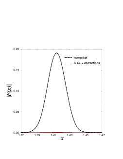
Figure 4: Comparison of the numerical $|F(x)|$ (dashed line) with the result from Eq. (7) (solid line). The two curves cannot be distinguished, this will also occur in all the following plots of the same type. We have taken here $\beta=5$, $k_{min}$ and $k_{max}$ being respectively the first and the $5000^{th}$ level. The peak corresponds to the length of the family shown in Fig. 3, $\ell=\sqrt{2}$ (in all the text, the hypotenuse of the triangle is chosen as unit length). The modulus of the difference between the numerical and analytical values of $F(x)$ is also plotted in this figure, but is barely seen on this scale (its largest value is $5\times 10^{-4}$). The usual semi-classical contribution (with only the first term of the r.h.s. of (7)) gives instead an error of about $10^{-2}$.

$\bullet$ We now concentrate on the second iterate of the family. Its contribution is less trivial than (7) and more generic ; hence we will present the computation in some details. One has here to consider double diffraction near the optical boundary. Eq. (5) is generalized to double (and in a similar fashion to multiple) diffraction :

$$G_{2}(\vec{r},\vec{r\,}^{\prime},E) = -2\int_{0}^{+\infty}\!\!\!ds\,G_{1}(\vec{s}\,,\vec{r\,}^{\prime},E)\,\vec{n}_{s}\cdot\vec{\nabla}_{\vec{s}\,}G_{0}(\vec{r},\vec{s}\,,E)$$ (9)

$$+ G_{1}(\vec{r}_{0},\vec{r\,}^{\prime},E)\,{\cal D}_{reg}(\theta,\theta^{\prime})\,G_{0}(\vec{r},\vec{r}_{0},E)\;,$$

where $G_{2}$ is the total (semi-classical plus diffractive) Green function.

When unfolding the trajectory (as done for instance in Fig. 3) near the diffractive boundary of the family, one is lead to consider contributions such as presented in Fig. 5. On that figure the position of a point $\vec{r}$ in vicinity of the diffractive trajectory on the boundary of the family is defined by coordinates $x$ and $y$. $x$ is a coordinate along the orbit ($0\leq x\leq\ell$) and $y$ a is transverse coordinate.

Figure 5: Schematic representation of the different contributions to the Green function $G_{2}$ near a diffractive periodic orbit on the boundary of the second iterate of a family. In this plot (and in the followings of the same type) the trajectory is represented after unfolding and the shaded areas are zones forbidden by classical mechanics. The path represented by a solid line going from $\vec{r}$ to $\vec{s}_{1}$, $\vec{s}_{2}$ and $\vec{r}$ contributes to the leading Kirchhoff term in the first integral of the r.h.s. of (9). The dashed path contributes at next order (it has one “Keller bounce” at $\vec{r}_{0}$ with diffraction coefficient ${\cal D}_{reg}$). Its contribution to the Green function corresponds to the second term in (14).

The leading order contribution of $G_{2}$ to the level density is the usual contribution of the second repetition of a family of periodic orbit. It is obtained by simply making the approximation $G_{2}\approx G_{0}$ and it is of the form :

$$\rho(E)\leftarrow{\displaystyle{\cal A}\over\displaystyle 2\pi}\frac{1}{\sqrt{\displaystyle 2\pi kL}}\,\cos(kL-\pi/4)\;.$$ (10)

Here and in the following of this section $L=n\,\ell$ is the total length of the trajectory, $\ell$ is the primitive length, and $n$ is the repetition number (here $n=2$).

The diffractive corrections to (10) are included into $\rho(E)$ through the following trace :

$$\rho(E)\leftarrow-\frac{1}{\pi}\,\mbox{Im}\,\int d^{2}r\,\left(G_{2}(\vec{r}\,,\vec{r}\,,E)-G_{0}(\vec{r}\,,\vec{r}\,,E)\right)\;.$$ (11)

From the expression (9) of $G_{2}$ one obtains the first order contribution to $G_{2}(\vec{r}\,,\vec{r}\,,E)-G_{0}(\vec{r}\,,\vec{r}\,,E)$ under the form :

$$\frac{\sqrt{\displaystyle k}\,{\mbox{\large e}}^{\displaystyle ikL+3i\pi/4}}{2\,(2\pi)^{3/2}\sqrt{\displaystyle x\ell(\ell-x)}}\!\!\!\! \left[\int_{0}^{+\infty}\!\!\!\!\!\!ds_{1}\int_{0}^{+\infty}\!\!\!\!\!\!ds_{2}\,\displaystyle{\mbox{\large e}}^{\displaystyle i\frac{\displaystyle k}{\displaystyle 2}\left\{\displaystyle\frac{\displaystyle(s_{1}-y)^{2}}{\displaystyle x}+\frac{\displaystyle(s_{2}-s_{1})^{2}}{\displaystyle\ell}+\frac{\displaystyle(y-s_{2})^{2}}{\displaystyle\ell-x}\right\}}\right.$$ (12)

$$-\!\!\!\! \Theta(y)\left.\int_{-\infty}^{+\infty}\!\!\!\!\!\!ds_{1}\int_{-\infty}^{+\infty}\!\!\!\!\!\!ds_{2}\,\displaystyle{\mbox{\large e}}^{\displaystyle i\frac{\displaystyle k}{\displaystyle 2}\left\{\displaystyle\frac{\displaystyle(s_{1}-y)^{2}}{\displaystyle x}+\frac{\displaystyle(s_{2}-s_{1})^{2}}{\displaystyle\ell}+\frac{\displaystyle(y-s_{2})^{2}}{\displaystyle\ell-x}\right\}}\right]\;.$$

This contribution corresponds to the main Kirchhoff term in (9) (i.e. to the solid path from $\vec{r}$ to $\vec{r}$ in Fig. (5)) from which the semi-classical contribution has been removed when it exists, i.e. when $y>0$ (this semi-classical contribution has been written as the double sum $\int_{-\infty}^{+\infty}ds_{1}\int_{-\infty}^{+\infty}ds_{2}$ in (12)). In the expression (12) one has made the hypothesis $|y-s_{1}|,|s_{1}-s_{2}|,|y-s_{2}|\ll x,\ell$. Thus, for instance, $|\vec{s}_{2}-\vec{s}_{1}|\simeq\ell+(s_{2}-s_{1})^{2}/(2\ell)$. The above expression has to be inserted into Eq. (11), i.e. integrated transverse to the orbit (along $y$) and longitudinally (along $x$). This is done in Appendix B and the resulting contribution to the level density is :

$$\rho(E)\leftarrow-\frac{\ell}{8\pi^{2}k}\,\cos(kL)\;.$$ (13)

This shows that the main diffractive correction to the contribution of the second iterate of a family is of order of the one of an isolated periodic orbit. Such non-generic contributions in vicinity of a family have already been studied in a slightly different context in Ref. [16].

For a better agreement with numerical data, one needs to include also the next order correction to (13) in the level density. This is done by including mixed Kirchhoff-Keller contributions in the Green function (9), such as described by the path represented in Fig. (5) by a dashed line. Along that path, the first diffraction at $\vec{r}_{0}$ is of Keller-type (involving a coefficient ${\cal D}_{reg}$), and the second one of Kirchhoff type (with an integral along $s_{2}$). One has two contributions, one for each possible location of Keller diffraction (a single one being shown in Fig. (5)). The relevant contribution to $G_{2}$ are now of the form :

$$\frac{{\cal D}_{reg}\,{\mbox{\large e}}^{\displaystyle ikL+i\pi/4-i\nu_{d}\pi/2}}{4\,{\sqrt{\displaystyle k}\,(2\pi)^{3/2}\sqrt{\displaystyle x\ell(\ell-x)}}}\left[\int_{0}^{+\infty}\!\!\!\!\!\!ds_{1}\,{\mbox{\large e}}^{i\frac{k}{2}\left\{\frac{(s_{1}-y)^{2}}{x}+\frac{s_{1}^{2}}{\ell}+\frac{y^{2}}{\ell-x}\right\}}+\int_{0}^{+\infty}\!\!\!\!\!\!ds_{2}\,{\mbox{\large e}}^{i\frac{k}{2}\left\{\frac{y^{2}}{x}+\frac{s_{2}^{2}}{\ell}+\frac{(y-s_{2})^{2}}{\ell-x}\right\}}\right]\;.$$ (14)

The integral of this expression is computed in Appendix B (Eq. (B10)). It yields the next correction to (13) which is of the form :

$$\rho(E)\leftarrow\frac{\ell}{2\pi k}\,\frac{{\cal D}_{reg}}{\sqrt{8\pi kL}}\,\cos(kL-\nu_{d}\pi/2-3\pi/4)\;.$$ (15)

In (15) $\nu_{d}$ is the Maslov index of the orbit corresponding to the dashed path in Fig. 5. If $\sigma$ is the relevant index near the optical boundary considered (i.e. the one for which ${\cal D}_{\sigma,\eta}$ in Eq. (3) diverges), one can show that $\exp\{-i\nu_{d}\pi/2\}=\sigma$.

There is a last correction to (15), purely of Keller-type, giving a contribution of order ${\cal O}(k^{-2})$, but the contributions (10), (13) and (15) already give a very good description of the Fourier transform of the spectrum. This can be checked in Fig. 6 for the second iterate of the family drawn in Fig. 3.

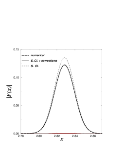
Figure 6: Same as Fig. 4 for the second iterate of the family. The solid curve (labelled “S. Cl. + corrections”) corresponds to Eqs. (10,13,15). In this plot and in the followings of the same type, we represent with a thin dashed line (denoted “S. Cl.”) the usual semiclassical result without diffractive corrections (which corresponds here to Eq. (10) alone). The modulus of the difference between the numerical and analytical $F(x)$ is also plotted in this figure, but is barely seen on this scale ; its largest value is $5\times 10^{-4}$, whereas the usual semi-classical approach gives an error of $1.4\times 10^{-2}$.

A simple remark is in order here : Eq. (10) is actually the first term of an expansion in $k^{-1}$ (or equivalently in $\hbar$). The magnitude of the next correction can be estimated by the following argument : the exact Green function in an infinite wedge can be expressed in terms of a Hankel function (with diffractive corrections unimportant for the present discussion) and this yields instead of Eq. (10) to something like

$$\rho(E) \leftarrow \frac{{\cal A}}{4\pi}J_{0}(kL)$$ (16)

$$\approx {\displaystyle{\cal A}\over\displaystyle 2\pi}\frac{1}{\sqrt{\displaystyle 2\pi kL}}\,\cos(kL-\pi/4)+\frac{\ell}{2\pi k}\,\frac{{\cal A}/(8\,L^{2})}{\sqrt{8\pi kL}}\,\sin(kL-\pi/4)+...$$

Equation (16) is the exact contribution of a family in an integrable polygon. Therefore there are non-diffractive corrections to the leading order (10) of the trace formula which are of same order as (15). To ${\cal D}_{reg}$ in (15) one simply adds a factor ${\cal O}({\cal A}/L^{2})$ (see the last term of the r.h.s. of (16)). In all our numerical checks this correction appeared to be negligible. By comparing the diffractive corrections with (16) one can note that : (i) the first diffractive term (13) is the leading $\sqrt{\hbar}$ correction in the trace formula and (ii) for long orbits (or large repetition number) the term ${\cal A}/L^{2}$ in (16) will be dominated by ${\cal D}_{reg}$ in (15).

$\bullet$ The determination of the contribution of the next iterates of a primitive family of periodic orbits with a diffractive boundary is patterned on the above derivation. We just state here the results.

The main contribution is the generic semi-classical one, of the form (10). The first correction is of a type similar to the contribution to the trace formula of an isolated periodic orbit :

$$\rho(E)\leftarrow-\frac{\ell}{\pi k}\,C_{n}\cos(kL)\;,$$ (17)

where $\ell$ is the primitive length, $n$ is the repetition number, $L=n\,\ell$ and $C_{n}$ is a dimensionless parameter given by the formula $C_{n}=(1/8\pi)\sum_{q=1}^{n-1}[q(n-q)]^{-1/2}$. We show how to compute it in some special cases in Appendix B and in general in Appendix D. Its first values are $C_{1}=0$, $C_{2}=1/(8\,\pi)$, $C_{3}=1/(4\pi\sqrt{2})$ … and it has the limiting value $C_{\infty}=1/8$.

The next correction to (17) is of the form (15). This is proven in special cases in Appendix B (Eqs. (B10,B11)) and in general in Appendix C.

We have tested the excellent agreement of contributions (10,17,15) with the numerical spectrum. We illustrate this for the fifth iterate of the family shown in Fig. 7. This family is particular in the sense that one of its boundaries is formed by an isolated orbit which has an extra bounce compared to the family ; it lies along the lower edge of the triangles in Fig. 7. The contribution of such an isolated orbit has been known for some time [24, 25] and is taken into account in the comparison with numerical results displayed in Fig. 8. The other boundary is a diffractive orbit of the type we are interested in. Its contribution to the level density is described by Eqs. (17,15).

Figure 7: Representation of a family of periodic orbits in the triangle $(\pi/2,\pi/8,3\pi/8)$ by the technique of unfolding. The family has a length $\ell=2\cos\pi/8$. Its area is shaded and the diffractive point on its boundary is marked with black dots.

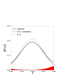
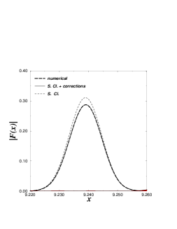
Figure 8: Same as Fig. 4 for the fifth iterate of the family shown in Figure 7 ($L\simeq 9.239$). The analytical result corresponds to Eqs. (10,17,15) with $n=5$. The modulus of the difference between the numerical and analytical $F(x)$ is represented by the shaded area. It is important on the left plot, due orbits in vicinity of the peak that are not taken into account. This overlapping of peaks can be suppressed by increasing $k_{max}$ (in order to decrease the width of the peaks in $|F(x)|$). This is done on the right plot which is drawn for $k_{max}$ corresponding to the 20 000^th level. Then, the largest discrepancy with the numerical result is $4\times 10^{-4}$ whereas the error when employing the usual semiclassical approach is 100 times larger.

$\bullet$ The following diffractive corrections to the contributions (10,17,15) to the $n^{th}$ iterate of a family correspond to orbits having $n_{k}$ Kirchhoff diffractions and $n_{g}$ Keller ones, with $n_{k}+n_{g}=n$. They yield corrections of order ${\cal O}(k^{-\frac{n_{g}+1}{2}})$ compared to the leading term (10). One can show that their contribution to the level density is of the form :

$$\rho(E)\leftarrow\frac{\ell}{2\pi k}\left(\frac{D_{reg}}{\sqrt{8\pi k\ell}}\right)^{n_{g}}B^{(n_{g})}_{n}\,\cos(kL-3n_{g}\pi/4-\nu_{d}\pi/2)\;.$$ (18)

The Maslov index $\nu_{d}$ in (18) is related to the index $\sigma$ of the optical boundary considered (i.e. the one for which ${\cal D}_{\sigma,\eta}$ in Eq. (3) diverges) by $\exp\{-i\nu_{d}\pi/2\}=\sigma^{n_{g}}$. $B^{(n_{g})}_{n}$ is a dimensionless coefficient. $B^{(1)}_{n}=n^{-1/2}$ (in agreement with (15)), $B^{(2)}_{n}=\sum_{q=1}^{n-1}q^{-3/2}(n-q)^{-1/2}$ and the general form is :

$$B^{(n_{g})}_{n}=\sum_{\{q_{i}\}}\;\prod_{i=1}^{n_{g}}\;(q_{i+1}-q_{i})^{-3/2}\;,$$ (19)

with the convention $q_{n_{g}+1}=n+q_{1}$. The sum is extended over all possible sets of $n_{g}$ integers $\{q_{i}\}_{1\leq i\leq n_{g}}$ with $1\leq q_{1}<q_{2}<...<q_{n_{g}}\leq n$.

4 A diffractive orbit on the frontier of both a family and of the billiard

In the previous Section we have studied the case that a diffractive periodic orbit lies on an optical boundary corresponding to the frontier of a family. There is a special configuration where such a diffractive orbit lies on two optical boundaries. From Fig. 1 one sees that two optical boundaries meet only on the edges defining the diffractive corner (when $\theta$ or $\theta^{\prime}=0$ or $\gamma$). Hence, in that case part of the diffractive trajectory crawls along the frontier of the billiard. This happens for instance for the diffractive trajectory on the boundary of the family shown on Fig. 10.

Although the diffractive periodic orbit considered bounds the first iterate of a family, it is already doubly diffractive. For incorporating such a configuration into the trace formula, one can still use Eqs. (5) and (9), but the semi-classical Green function to be incorporated in that formula has two contributions : one from the “direct” path (we call this path direct, but it may have bounces that are not materialized by the process of unfolding) and one from a path bouncing on the frontier of the billiard which is also the frontier of the family (see Fig. 10).

Figure 9: Representation of a family of periodic orbits in the triangle $(\pi/2,\pi/8,3\pi/8)$ by the technique of unfolding. The family has a length $L=(4+2\sqrt{2})^{1/2}\simeq 2.613$. Its area is shaded and the diffractive points on its boundary are marked with a black spot. The boundary of the family party coincides with the frontier of the billiard.

Figure 10: Schematic representation of the different contributions to the Green function near a diffractive periodic orbit on the boundary of a family. The boundary of the family coincides with the one of the billiard along a segment of length $\ell_{2}$. In this case, the main Kirchhoff term in (9) contains two paths which are represented with solid lines of the figure.

In that figure one has represented a configuration where a point in vicinity of the diffractive periodic orbit lies along the part of the boundary of the family which does not coincide with one frontier of the billiard (we denote by $\ell_{1}$ the length of this part, and by $\ell_{2}$ the length of the part along a frontier of the billiard, $\ell_{1}+\ell_{2}=L$). Then, the main Kirchhoff contribution to $G_{2}$ is of the form :

$$\frac{\sqrt{k}\,{\mbox{\large e}}^{ikL+3i\pi/4}}{2\,(2\pi)^{3/2}\sqrt{x\,\ell_{2}(\ell_{1}-x)}}\!\!\!\!\!\!\!\!\! \left[\int_{0}^{+\infty}\!\!\!\!\!ds_{1}\int_{0}^{+\infty}\!\!\!\!\!ds_{2}\,{\mbox{\large e}}^{i\frac{k}{2}\left\{\frac{(s_{1}-y)^{2}}{x}+\frac{(s_{2}-s_{1})^{2}}{\ell_{2}}+\frac{(y-s_{2})^{2}}{\ell_{1}-x}\right\}}\right.$$ (20)

$$- \left.\int_{0}^{+\infty}\!\!\!\!\!ds_{1}\int_{0}^{+\infty}\!\!\!\!\!ds_{2}\,{\mbox{\large e}}^{i\frac{k}{2}\left\{\frac{(s_{1}-y)^{2}}{x}+\frac{(s_{2}+s_{1})^{2}}{\ell_{2}}+\frac{(y-s_{2})^{2}}{\ell_{1}-x}\right\}}\right]\;.$$

The second contribution in (20) is obtained from the first one by the method of images. It corresponds in Fig. 10 to the path going from $\vec{s}_{1}$ to $\vec{s}_{2}$ with one bounce on the frontier of the billiard. If the point $\vec{r}\,$ of Fig. 10 lies along the part of the orbit coinciding with the frontier of the billiard, then the main Kirchhoff contribution to $G_{2}$ is a sum of four terms (this is detailed in Appendix B, cf. Fig. 24). We will not give the explicit computation here (see Appendix B), but after transverse integration along $y$ the final result for the first diffractive correction to the contribution of a family such as the one presented in Fig. 10 is :

$$\rho(E)\leftarrow-\frac{1}{4\pi^{2}k}\left(\sqrt{\ell_{1}\ell_{2}}+L\;\mbox{arctg}\,\sqrt{\frac{\displaystyle\ell_{2}}{\displaystyle\ell_{1}}}\,\right)\,\cos(kL)\;.$$ (21)

The next diffractive corrections to (21) are of the order of a doubly diffractive Keller correction, and we do not include them in our description of the family. As seen in Fig. 11, contributions (10) and (21) already give an excellent description of the Fourier transform of the spectrum in vicinity of the length of the family drawn on Fig. (10).

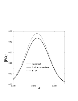
Figure 11: Comparison between the numerical evaluation of $F(x)$ with the result of Eqs. (10,21) for $x$ close to the length of the family shown in Fig. 10. The modulus of the difference is also plotted on the figure, but cannot bee seen (it is lower than $10^{-3}$).

5 A diffractive orbit jumping from the boundary of a family to the boundary of an other one

In the billiard we consider, an interesting combination of orbits occurs. It is formed by the gathering of two diffractive orbits, each being on the boundary of a family, and where the total diffractive orbit is on the optical boundary, although the two families have no overlap. An example of such a case is given in Fig. 13.

Figure 12: Representation of a diffractive orbit that jumps from the boundary of a family to the boundary of an other one. The area occupied by each family is shaded. The first family transports triangle $A$ to position $B$, and the second one transports triangle $B$ to position $C$. The diffractive orbit is the thick solid line with its three diffractive points marked by black dots. It has a length $L_{d}=(10+7\sqrt{2})^{1/2}\simeq 4.461$.

Figure 13: Schematic representation of the contributions to the Green function in vicinity of a diffractive orbit that jumps from the boundary of a family to the boundary of another one (such as the one shown in Fig. 13). $\ell_{1}$ corresponds to the length of the family that maps triangle $B$ onto triangle $C$ in Fig. 13 and $\ell_{2}+\ell_{3}$ to the length of the family that maps triangle $A$ onto $B$. For this last family, $\ell_{2}$ is the length of the part of its boundary that lies along the frontier of the billiard.

As seen in Figure 13, although the diffractive orbit lies on the optical boundary, there is no allowed classical trajectory nearby. This type of orbit might be a particularity of Veech billiards, but it is nevertheless interesting to describe its contribution to the level density. The schematic representation of the neighborhood of the orbit is displayed in Fig. 13.

In the cases we have studied, the problem is complicated by the fact that one of the families considered has a boundary that partially coincides with the frontier of the billiard, i.e. is of the type studied in the previous section. Hence, there are three relevant lengths along the orbit we consider : $\ell_{1}$ is the length of one of the families, $\ell_{2}+\ell_{3}$ is the length of the second one, $\ell_{2}$ being the length that corresponds to the part of the boundary of the second family lying along the frontier of the billiard.

The diffractive Green function to be considered here is of the the type previously studied in Section 4, with an additional diffractive bounce. Hence, one defines a Green function $G_{3}$ connected to $G_{2}$ in the same manner as $G_{2}$ is connected to $G_{1}$ in Eq. (9). Due to the possible bounce along the frontier of the billiard that coincides with the boundary of the family, the semi-classical Green function to be incorporated in this formula has several contributions. This is illustrated in Fig. 13 where there are two possible paths for going from $\vec{s}_{1}$ to $\vec{s}_{2}$ (such a contribution was already present in Fig. 10). If the initial point $\vec{r}\,$ were lying near the frontier of the billiard (next to the part of the family of length $\ell_{2}$), one would have four different paths : two for going from $\vec{r}\,$ to $\vec{s}_{2}$ and two for going from $\vec{s}_{1}$ to $\vec{r}\,$. After transverse integration of these four contributions (along the variable $y$), one can verify that they lead to the same contribution as the ones displayed in Fig. 13, hence we will only present here the computation in the simpler case shown in Fig. 13.

For the configuration of Fig. 13, the Kirchhoff term in the expression of $G_{3}$ reads :

$$(2ik)^{3}\,D_{3}(x,\ell_{1},\ell_{2},\ell_{3})\!\!\!\! \left[\int_{0}^{+\infty}\!\!\!\!\!ds_{1}\int_{0}^{+\infty}\!\!\!\!\!ds_{2}\int_{-\infty}^{0}\!\!\!\!\!ds_{3}\,{\mbox{\large e}}^{i\frac{k}{2}\left[\frac{(s_{1}-y)^{2}}{x}+\frac{(s_{2}-s_{1})^{2}}{\ell_{2}}+\frac{(s_{3}-s_{2})^{2}}{\ell_{3}}+\frac{(y-s_{3})^{2}}{\ell_{1}-x}\right]}\right.$$ (22)

$$-\!\!\!\! \left.\int_{0}^{+\infty}\!\!\!\!\!ds_{1}\int_{0}^{+\infty}\!\!\!\!\!ds_{2}\int_{-\infty}^{0}\!\!\!\!\!ds_{3}\,{\mbox{\large e}}^{i\frac{k}{2}\left[\frac{(s_{1}-y)^{2}}{x}+\frac{(s_{2}+s_{1})^{2}}{\ell_{2}}+\frac{(s_{3}-s_{2})^{2}}{\ell_{3}}+\frac{(y-s_{3})^{2}}{\ell_{1}-x}\right]}\right]\;,$$

where the notation $D_{n}$ is defined in Appendix B. In (22), the second term of the r.h.s. is obtained from the first one by the method of image. It corresponds to a path going from $\vec{s}_{1}$ to $\vec{s}_{2}$ with a specular bounce off the frontier of the billiard (cf. Fig. 13). Note that there is no classical path contributing to (22) : it is clear from Fig. 13 that there exits no classical trajectory from $\vec{r}\,$ to $\vec{r}\,$. The transverse and longitudinal integrations are done in a manner similar to the one exposed in Appendix B for the similar case of an orbit which boundary coincides with the frontier of the billiard (cf. Section 4). The contribution of the diffractive orbit to the level density is :

$$\rho(E)\leftarrow-\frac{L_{d}}{8\pi^{2}k}\,\cos(kL_{d})\left\{\,\mbox{arctg}\,\sqrt{\frac{\displaystyle\ell_{2}}{\displaystyle\ell_{3}+\ell_{1}}}\right.\!\!\!\! - \!\!\!\!\,\mbox{arctg}\,\sqrt{\frac{\displaystyle\ell_{3}+\ell_{2}}{\displaystyle\ell_{1}}}+\,\mbox{arctg}\,\sqrt{\frac{\displaystyle\ell_{3}}{\displaystyle\ell_{1}+\ell_{2}}}$$

$$-\frac{\sqrt{\displaystyle\ell_{3}(\ell_{1}+\ell_{2})}}{\displaystyle L_{d}}\!\!\!\! + \!\!\!\!\left.\frac{\sqrt{\displaystyle\ell_{2}(\ell_{3}+\ell_{1})}}{\displaystyle L_{d}}-\frac{\sqrt{\displaystyle\ell_{1}(\ell_{2}+\ell_{3})}}{\displaystyle L_{d}}\right\}\;,$$ (23)

where $L_{d}=\ell_{1}+\ell_{2}+\ell_{3}$ is the length of the diffractive orbit.

In order to have a good description of the contribution of the orbit we are considering here, one needs (as in Section 3) to incorporate next order corrections, i.e. mixed Kirchhoff-Keller terms. This corresponds in Fig. 13 to the path with one Keller bounce on the apex which is not on the frontier of the billiard (dashed line) (Keller bounces on the other apexes contribute to higher order). We do not detail the computation here and just present the resulting correction to (5). It is of the form :

$$\rho(E)\leftarrow\frac{L_{d}}{2\pi^{2}k}\,\frac{\displaystyle{\cal D}_{reg}}{\sqrt{\displaystyle 8\pi kL_{d}}}\,\mbox{arctg}\,\sqrt{\frac{\displaystyle\ell_{3}\ell_{1}}{\ell_{2}L_{d}}}\,\cos(kL_{d}-\nu_{d}\pi/2-3\pi/4)\;.$$ (24)

As one can see in Fig. 14, Eqs. (5,24) give an excellent account of the contribution to the level density of the orbit shown on Fig. 13.

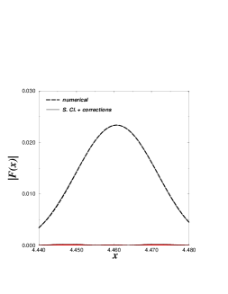
Figure 14: Same as Fig. 4 for the orbits shown of Fig. 13. The solid line corresponds to the results of Eqs. (5,24). The shaded area at the bottom corresponds to the modulus of the difference between the numerical and the analytical result (which is inferior to $2\times 10^{-4}$). Note that the standard semi-classical approach completely misses this peak in $|F(x)|$.

6 A diffractive orbit bouncing between the upper and lower boundary of a family

Up to now we have only considered diffractive orbits which were lying exactly on the optical boundary. Other types of diffractive orbit occur which do not stand right on the optical boundary, but close enough to prevent their description by the geometrical theory of diffraction. Such an orbit is represented in Fig. 16.

Figure 15: A diffractive orbit on the boundary of a family (straight line between two black dots). The family is not represented, but it connects the upper left triangle to the lower right one. The other orbit shown is typical of those studied in this section. It is a doubly diffractive orbit close to the family, it is represented by the segmented line between three black dots.

Figure 16: Graphical representation of different diffractive contributions for a family limited by two opposite wedges. The leading term in (9) corresponds to the solid line. The dashed path is one of the next order corrections, involving one Keller bounce (with a coefficient ${\cal D}_{reg}$) on one of the apexes. $\zeta$ is the distance between the two apexes measured transverse to the direction of the family.

On this Figure, the upper left triangle and the lower right one are connected by a family. For legibility we do not represent it and its area. We only represent the diffractive orbit on its boundary (the straight line between two black dots). This orbit is singly diffractive and its contribution corrects the one of the family as in Eq. (7). There is a diffractive orbit nearby, not exactly on the optical boundary, but very close to being part of the family : it starts and ends at the same point as the diffractive orbit on the boundary of the family, but it has an extra diffractive bounce in between (see Figure 16). This is the type of orbits we aim to describe in this section. Its diffraction coefficient does not exactly diverge, but one of the contributions ${\cal D}_{\sigma,\eta}$ of (3) is large and does not allow a proper description of the diffractive Green function by means of Eq. (2). For simplicity we will denote this part as the “divergent part” (the remaining being the “regular part”).

The configuration we just described is of the type represented schematically on Fig. 16. The projection of the upper diffractive corner onto the family separates it in two parts of lengths $\ell_{1}$ and $\ell_{2}$ ($\ell_{1}+\ell_{2}=L$). Typically, the upper wedge represented in that figure is the upper boundary of the family. In that case, if $\zeta$ denotes the distance from the upper wedge to the lower extend of the family, the area occupied by the family is simply ${\cal A}=\zeta\,L$ ($L$ being the length of the family, see Figure 16).

In this configuration the leading term in the Green function is obtained from the explicit expression of $G_{2}$ and reads :

$$G_{2}(\vec{r}\,,\vec{r}\,,E)\approx\frac{\sqrt{\displaystyle k}\,{\mbox{\large e}}^{\displaystyle ikL+3i\pi/4}}{2\,(2\pi)^{3/2}\sqrt{\displaystyle x\ell_{2}(\ell_{1}-x)}}\;\int_{-\infty}^{\zeta}\!\!\!\!\!ds_{1}\int_{0}^{+\infty}\!\!\!\!\!ds_{2}\;{\mbox{\large e}}^{i\frac{k}{2}\left\{\frac{(s_{1}-y)^{2}}{x}+\frac{(s_{2}-s_{1})^{2}}{\ell_{2}}+\frac{(y-s_{2})^{2}}{\ell_{1}-x}\right\}}\;.$$ (25)

The above expression integrated transversely (along $y$) and longitudinally (along $x$) gives the contribution of the family and of its corrections to the level density. The result reads (the relevant integrals are given in Appendix B)

$$-\frac{1}{\pi}\,\mbox{Im}\,\int d^{2}r\,G_{2}(\vec{r}\,,\vec{r}\,,E) \approx {\displaystyle{\cal A}\over\displaystyle 2\pi}\frac{1}{\sqrt{\displaystyle 2\pi kL}}\,\cos(kL-\pi/4)$$ (26)

$$+\frac{\sqrt{\displaystyle\ell_{1}\ell_{2}}}{\displaystyle 4\pi^{2}\,k} \left[\cos(kL_{d})-2\,\sqrt{\pi k\Delta}\;\mbox{Re}\,\left\{{\mbox{\large e}}^{ikL_{d}-i\pi/4}K\left(\sqrt{k\Delta}\right)\right\}\right]\;.$$

In (26), $K$ is the modified Fresnel function defined in Appendix A. We have denoted by $L_{d}$ the length of the doubly diffractive orbit going from the upper corner to the lower one ($L_{d}=\sqrt{\ell_{1}^{2}+\zeta^{2}}+\sqrt{\ell_{2}^{2}+\zeta^{2}}$), by $\Delta$ the length difference $L_{d}-L$, and have made the approximation $\Delta\simeq\zeta^{2}L/(2\ell_{1}\ell_{2})$. The first term of the r.h.s. of (26) is the usual contribution of a family. The second is a diffractive correction.

Two remarks are in order here :

$\bullet$ It may happen that the upper corner of Fig. 16 does not provide the upper boundary of the family because the family meets an other non-diffractive boundary between the two diffractive corners. This is the case presented in Fig. 16 ; the family does not occupy all the width between the two diffractive corners : it meets first a non-diffractive $\pi/2$ corner. In this case formula (26) remains valid, but ${\cal A}=\zeta\,L/2$.

$\bullet$ Secondly, it is interesting to check what is the behavior of Eq. (26) when the two wedges are far apart, i.e. in the limit $\sqrt{k\Delta}\gg 1$. By using the asymptotic expansion (A3) of the modified Fresnel function one obtains :

$$-\frac{1}{\pi}\,\mbox{Im}\,\int d^{2}r\,G_{2}(\vec{r}\,,\vec{r}\,,E) \underset{\sqrt{k\Delta}\gg 1}{\approx} {\displaystyle{\cal A}\over\displaystyle 2\pi}\frac{1}{\sqrt{\displaystyle 2\pi kL}}\,\cos(kL-\pi/4)$$ (27)

$$+\frac{L_{d}}{2\pi k}\left(\frac{2\ell_{1}\ell_{2}}{L_{d}\Delta}\right)\frac{1}{8\pi k\sqrt{\ell_{1}\ell_{2}}}\cos(kL_{d}-3\pi/2)\;.$$

In (27), to the usual contribution of a family is added a term which can be matched with a contribution such as (4) with two diffractive bounces, provided some approximations are made. The term $2\ell_{1}\ell_{2}/(L_{d}\Delta)$ stands were one would expect a product of two coefficients ${\cal D}$. Indeed, one can show that this term corresponds to the product of the two divergent parts ${\cal D}_{\sigma,\eta}$ near the optical boundary. But it is not of the form (3) which is the only acceptable in the limit where Eq. (27) has been written (i.e. far from the optical boundary). This is a well known drawback of Kirchhoff’s approximation already discussed in Section 2.2. It can be cured relatively easily : if the optical boundary close to the diffractive orbit is characterized by the indices $\sigma$ and $\eta$, one has to multiply the second terms of the r.h.s. of (26) by the factor $(|a^{d}_{\sigma,\eta}|\,{\cal D}^{d}_{\sigma,\eta})^{2}/2$ and to express $\Delta$ as $|a^{d}_{\sigma,\eta}|^{2}\ell_{1}\ell_{2}/L_{d}$ (instead of $L_{d}-L$). The term $a_{\sigma,\eta}$ appearing in these expressions is defined in Eq. (A4). The upper index $d$ is meant to remind that $a_{\sigma,\eta}$ and ${\cal D}_{\sigma,\eta}$ have to bee evaluated on the diffractive periodic orbit of length $L_{d}$. This procedure allows recovery of the correct limit in (27). Moreover it does not affect (26) when the diffractive orbit is close to the family (i.e. in the limit $\sqrt{k\Delta}\ll 1$) since in this limit $(|a^{d}_{\sigma,\eta}|\,{\cal D}^{d}_{\sigma,\eta})^{2}/2\simeq 1$ and $\Delta\simeq|a^{d}_{\sigma,\eta}|^{2}\ell_{1}\ell_{2}/L_{d}$.

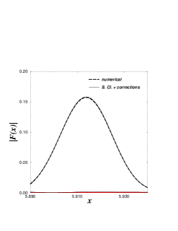
Figure 17: Same as Fig. 4 for the orbits shown on Fig. 16. The solid line corresponds to Eqs. (26,28). Here one has $L=(1+\sqrt{2})\sqrt{6}\simeq 5.9136$ and $L_{d}=(10+3\sqrt{2})^{1/2}+(6-\sqrt{2})^{1/2}\simeq 5.9154$. The shaded area hardly seen at the bottom of the plot corresponds to the modulus of the difference between the numerical and the analytical result (which is inferior to $1.4\times 10^{-3}$). The pure semi-classical estimate (Eq. (10)) gives an error of $4.6\times 10^{-2}$. Taking only into account the diffractive periodic orbit standing exactly on the boundary of the family (as in Eq. (7)) gives an even larger error ($5.3\times 10^{-2}$).

Eq. (26) is not the final contribution from the configuration represented in Figure 16. This is clear from (27) : far from the optical boundary the asymptotic evaluation of (26) only allows to recover the divergent part of the diffraction coefficient. Hence one has to include other terms, of mixed type Keller-Kirchhoff, as already encountered in Sections 3 and 5. These involve the regular part ${\cal D}_{reg}$ of the diffraction coefficients. We must be careful though, that one has now two different diffraction coefficients : one for the orbit along the boundary of the family (we denote it by ${\cal D}_{reg}^{f}$) and an other one for the orbit bouncing from the lower wedge to the upper one (we denote it by ${\cal D}_{reg}^{d}$). The remaining contribution to $\rho(E)$ of the configuration considered in this section is (we do not detail the derivation) :

$$\rho(E) \leftarrow \frac{L}{2\pi k}\frac{\displaystyle{\cal D}^{f}_{reg}}{\sqrt{\displaystyle 8\pi kL}}\,\cos(kL-\nu_{d}\pi/2-3\pi/4)$$ (28)

$$+ \frac{L}{\pi k}\frac{\displaystyle{\cal D}^{d}_{reg}}{\sqrt{\displaystyle 8\pi kL}}\,\mbox{Re}\,\left\{{\mbox{\large e}}^{ikL_{d}+i\pi/4}K\left(\sqrt{k\Delta}\right)\right\}$$

$$+ \frac{L_{d}}{2\pi k}\frac{\left({\cal D}_{reg}^{d}\right)^{2}}{8\pi k\sqrt{\ell_{1}\ell_{2}}}\cos(kL_{d}-3\pi/2)\;.$$

The term involving a modified Fresnel function in the above expression can be made uniform by a procedure similar to the one devised for Eq. (26). Note also that we have added in (28) a doubly diffractive term of purely Keller type (last term of the r.h.s.). It is a small correction and such terms were neglected in the previous sections. We kept it here for consistency because far from the optical boundary, it is of same order as the second term of the r.h.s. of (26).

The agreement with the numerical spectrum is here also excellent, as shown by Figure 17. Note that the geometrical theory of diffraction – although yielding a non-divergent result – is completely inadequate in this case. It amounts here to treating the isolated diffractive orbit as truly isolated from the family : hence to describing the family of periodic orbits in the usual way (i.e. using Eq. (10)) and including a correction of type (4) describing the contribution of the doubly diffractive orbit bouncing between the upper and lower boundary of the family. This procedure gives an error of $9.4\times 10^{-2}$ in Fig. 17.

7 A diffractive orbit near an isolated one

In this Section we will study, as in the previous one, a diffractive orbit standing not exactly on the optical boundary, but close to an allowed ‘periodic orbit. Here we consider the case that the nearby orbit is an isolated one (and not part of a family as in the previous section). Such a configuration has already been studied in Ref. [17], and we will here re-derive the result in a simpler manner (but with less generality).

A typical occurrence of the situation we are interested in is shown on Fig. 19. The isolated orbit we consider is the third iterate of the shortest classical periodic orbit of the system. It has a length $L=3/\sqrt{2}\simeq 2.121$. The nearby singly diffractive orbit has a length $L_{d}=(6-\sqrt{2})^{1/2}\simeq 2.141$.

Figure 18: A diffractive orbit (straight line between two black points) near an isolated orbit (straight line connecting two corners with opening angle $\pi/2$).

Figure 19: In this figure the isolated periodic orbit connects the two open circles. A nearby path from $\vec{r}\,$ to $\vec{r}\,$ is represented. There is an inversion along the periodic orbit for the transverse coordinate $y$ (see the text). The diffractive periodic orbit goes from one open circle to the apex at $\vec{r}_{0}$ and to the other open circle. It has a length $L_{d}\simeq L+2\zeta^{2}/L$.

The different contributions to the Green function $G_{1}$ are illustrated in Fig. 19. Note that for the phase-space coordinate transverse to the direction of an orbit, a bounce on a straight segment leads to an inversion. Hence, in a polygonal enclosure, the transverse mapping near a periodic orbit is either an inversion (for an odd number of bounces) and the orbit is then isolated, or the identity (for an even number of bounces) and the orbit is then part of a family. This is the reason for the inversion on Fig. 19 of point $\vec{r}\,$ with respect to the axis of the isolated periodic orbit after the process of unfolding. In the Figure, $\zeta$ is the distance from the diffractive apex to the periodic orbit.

In the case of interest here, the Kirchhoff part of the total Green function $G_{1}$ is (from Eq. (5) and Fig. 19) :

$$-\frac{{\mbox{\large e}}^{\displaystyle ikL-i\nu\pi/2}}{4\pi\sqrt{x(L-x)}}\,\int_{0}^{+\infty}\!\!\!\!\!ds_{1}\,\exp\left\{i\frac{k}{2}\left[\frac{(y+\zeta-s_{1})^{2}}{x}+\frac{(\zeta-y-s_{1})^{2}}{L-x}\right]\right\}\;,$$ (29)

where $\nu$ is the Maslov index of the isolated orbit ($\exp\{i\nu\pi/2\}=-1$). If $\nu_{d}$ is the one of the diffractive orbit and if $\sigma$ characterizes the nearby optical boundary, one has $\exp\{i\nu_{d}\pi/2\}=\sigma\exp\{i\nu\pi/2\}$. Once $G_{0}$ has been removed, the above expression yields – after transverse and longitudinal integration – the main contribution of the diffractive orbit to the level density. There is also a corrective term containing the regular part of the diffraction coefficient. Altogether one obtains the following contribution :

$$\rho(E)\leftarrow\frac{-L}{4\pi k}\,\mbox{Re}\,\left\{{\mbox{\large e}}^{ikL_{d}-i\nu\pi/2}K\left(\sqrt{k\Delta}\right)\right\}+\frac{L_{d}}{2\pi k}\frac{\displaystyle{\cal D}_{reg}}{\sqrt{\displaystyle 8\pi kL_{d}}}\,\cos(kL_{d}-\nu_{d}\pi/2-3\pi/4)\;,$$ (30)

where $\Delta=L_{d}-L\simeq 2\zeta^{2}/L$. As in the previous section we have used a representation of the Green function based on Kirchhoff’s approximation which does not yield a uniform formula : Eq. (30) does not permit recovery of the result of the geometrical theory of diffraction far from the optical boundary, i.e. when the isolated and the diffractive orbit are far apart. As in Section 6, one can easily remedy this deficiency. If the optical boundary to which the diffractive orbit is close is characterized by the indices $\sigma$ and $\eta$, one multiplies the first term of the r.h.s. of (30) by $\sigma(L_{d}/L)|a_{\sigma,\eta}|\,{\cal D}_{\sigma,\eta}/\sqrt{2}$ and replaces $\sqrt{\Delta}$ in the argument of the modified Fresnel function by $|a_{\sigma,\eta}|\,\sqrt{L_{d}}/2$. This procedure does not affect (30) in the limit that the diffractive and isolated periodic orbits are close and it allows recovery of the result of the geometrical theory of diffraction when these two orbits are well separated.

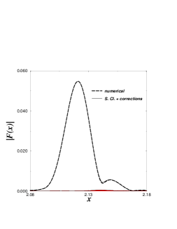
Figure 20: Same as Fig. 4 for the orbits shown on Fig. 19. The solid line corresponds to the contribution of the isolated diffractive orbit (which has a length $L=3/\sqrt{2}\simeq 2.121$) plus the contribution of the nearby diffractive orbit ($L_{d}=(6-\sqrt{2})^{1/2}\simeq 2.141$). The shaded area at the bottom of the plot corresponds to the modulus of the difference between the numerical and the analytical result (which is inferior to $5\times 10^{-4}$). We have used here the uniformized version of Eq. (30) (see the text), the use of the plain formula gives twice a larger discrepancy with numerical datas.

The comparison of formula (30) with the numerical result is very good, as shown in Fig. 20. Note that the geometrical theory of diffraction is not totally inadequate here (as it was in the previous section). It gives an error only four times larger than our approach. The reason is that the classical and diffractive orbits considered here are not very close to each other. Of course, the distance between two orbits must be measured relatively to the wave length. As a result the accuracy of the geometrical theory of diffraction depends on the window of the spectrum chosen for evaluating $F(x)$. For instance, evaluating $F(x)$ keeping only the first 500 levels (instead of the first 5000 levels as in Fig. 20) gives for the geometrical theory of diffraction an error 10 times larger than our approach.

8 A rectangular billiard with a flux line

In this Section we depart from the previous examples which treat corner diffraction, and we consider instead diffraction by a flux line. We consider a rectangular billiard (with sides of length $a$ and $b$) with a flux line located at point $\vec{r}_{0}$ inside the billiard (cf. Fig. 21a).

We will not restart here a detailed study of a large number of different cases of diffraction in the system (as was done in Secs. 2 to 7 for a triangular billiard). First, because Aharonov-Bohm diffraction is in a sense simpler than corner diffraction and leads to fewer exceptional cases ; second because we chose this example merely to illustrate the flexibility of Kirchhoff’s approach devises in Sec. 2. We will show that Eq. (6) permits to tackle the problem of multiple forward Aharonov-Bohm scattering.

Figure 21: Part (a) : the rectangular billiard and the two bouncing ball orbits (the vertical and the horizontal one). The flux line is located at point $\vec{r}_{0}$ marked by a white circle. Part (b) : representation of the typical contribution to the Green function (6) in vicinity of the doubly diffractive orbit belonging to one of the bouncing ball families. The path going from $\vec{r}$, to $\vec{s}_{1}$, $\vec{s}_{2}$ and back to $\vec{r}$ represented in the figure accumulates a phase $\exp(-2i\pi\alpha)$) (see the text).

This problem is encountered for instance when evaluating the contribution to the trace formula of the two families drawn in Fig. 21a. For each of these families the periodic orbit that encounters the point $\vec{r}_{0}$ twice on its way gives a doubly diffractive contribution. The schematic contribution to (6) for a nearby closed path is illustrate in Fig. 21b. In this Figure there is a reflection on the frontier of the billiard between the two flux lines and this has the effect of changing the sign of $\alpha$ on the second flux line (equivalently one could keep the same $\alpha$ and change the orientation of the axis $(\vec{r}_{0},s_{2})$). From Eq. (6) the diffractive Green function of the problem is written :

$$G_{2d}(\vec{r},\vec{r},E) = \frac{\sqrt{k}\,{\mbox{\large e}}^{i(k\ell-\pi/2)}}{2\pi\sqrt{8\pi x\ell_{2}(\ell_{1}-x)}}$$

$$\int_{-\infty}^{+\infty}\!\int_{-\infty}^{+\infty}\!\!\!\!\!ds_{1}ds_{2}\;{\mbox{\large e}}^{\frac{ik}{2}\left\{\frac{(y-s_{1})^{2}}{x}+\frac{(s_{2}-s_{1})^{2}}{\ell_{2}}+\frac{(y-s_{2})^{2}}{\ell_{1}-x}\right\}}\left[{\mbox{\large e}}^{i\pi\alpha\{\mbox{\small sgn}\,(s_{1})-\,\mbox{\small sgn}\,(s_{2})\}}-1\right]\;,$$

where $\ell$ is the length of the periodic orbit. The flux line (encountered twice) separates the orbit in three parts having lengths denoted by $x$, $\ell_{2}$ and $\ell_{1}-x$ in (8) and Fig. 21b ($\ell_{1}+\ell_{2}=\ell$). Transverse integration yields :

$$\int_{-\infty}^{+\infty}\!\!\!\!\!dy\;G_{2d}(\vec{r},\vec{r},E)=-\frac{\sqrt{\ell_{1}\ell_{2}}}{2\pi k\ell}\;{\mbox{\large e}}^{\displaystyle ik\ell+i\pi/2}\left\{\cos(2\pi\alpha)-1\right\}\;,$$ (32)

and this gives a contribution to the level density :

$$\rho(E)\leftarrow-\frac{\sqrt{\ell_{1}\ell_{2}}}{\pi^{2}k}\sin^{2}(\pi\alpha)\cos(k\ell)\;.$$ (33)

We check in Fig. 22 the very good agreement with the Fourier transform of the spectrum in vicinity of the length of the families drawn on Fig. 21a. In this Figure, the numerical $F(x)$ is computed using Eq. (8) with $\beta=5$, $k_{min}$ and $k_{max}$ being respectively the first and the $1400^{th}$ level. In the numerical computation we took $\alpha=1/2$ because in this case the diffractive effects on the level density are at maximum (see Eq. (33)). The shaded area hardly seen at the bottom of the plot is the modulus of the difference between the numerical and analytical $F(x)$. For obtaining the excellent agreement of Fig. 22 we have taken into account classical isolated boundary orbits (of the type already encountered for the family drawn in Fig. 7) and simple nearby diffractive periodic orbits which can be treated within the geometrical theory of diffraction (the relevant formulae are given in [26]). Not taking into account the diffractive contribution (33) would give a much larger error which is represented by a thin dashed line.

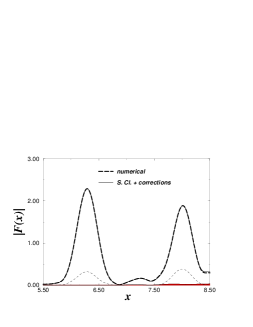
Figure 22: Comparison of the numerical $|F(x)|$ (dashed line) with the result from Eqs. (10,33) (solid line). The large peaks correspond to the lengths of the families shown in Fig. 21a. In our computations we have taken the sides of the rectangle to be $a=4$ and $b=\pi$ and the bouncing ball families have then a length $\ell=8$ and $2\pi$. The shaded line barely seen at the bottom is the modulus of the difference between the numerical and analytical $F(x)$. We also show as a thin dashed line the value of this difference when not including the contribution (33).

9 Conclusion

In this paper we have studied diffractive corrections to the semiclassical trace formula for the level density of polygonal billiards. Special care has been devoted to the treatment of diffractive periodic orbits lying on (or in vicinity of) the optical boundary, i.e. on the verge of being allowed by classical mechanics. In particular we derived a systematic expansion for the corner-diffractive corrections to the $n^{th}$ iterate of a family of periodic orbits.

The method employed (based on approximation (5)) allows to treat a rich variety of different cases with great precision (Secs. 2 to 7). This method is easily extended to similar diffraction problems. In particular, our approach to the diffractive correction of the $n^{th}$ iterate of a family allows to treat the non-trivial problem of multiple forward Aharonov-Bohm diffusion (Sec. 8).

The main purpose of our study was to establish the basis of a trace formula in pseudo-integrable systems, with contributions from diffractive orbits. It seems that these diffractive corrections are responsible for particular forms of spectral statistics observed in many such models [11]. Further investigations will elucidate this relationship.

Acknowledgments

It is a pleasure to thank M. Sieber for fruitful comments on the manuscript and for bringing Ref. [20] to our attention.

Appendix A

In this Appendix we derive Kirchhoff-like formulae for the Green function in the cases of corner and flux line diffraction (Eqs. (5,6)). Here we compare Eqs. (5) and (6) with the exact diffraction in the free plane : diffraction by an infinite wedge (in Appendix A.1) and by a flux line in the plane (in Appendix A.2). Adding boundaries to the problem (e.g. putting the flux line in a billiard) amounts – through the method of images – to add other sources of diffraction. In this case we describe multiple diffraction by using a natural generalization of Eqs. (5,6) (see e.g. Eq. (9)).

Appendix A.1 Corner diffraction

A uniform approximation for diffraction on a single corner has been first given by Pauli [21]. The subject has been studied in detail in the late 1960s and in the 1970s. We state here the result of one possible method of “uniformization” (detailed derivation and references can be found in [17]) :

$$G_{1d}(\vec{r},\vec{r\,}^{\prime},E)=\frac{1}{4}\,\frac{{\mbox{\large e}}^{ikL_{d}+i\pi/4}}{\sqrt{\pi kL_{d}}}\sum_{\sigma,\eta=\pm 1}|a_{\sigma,\eta}|\;{\cal D}_{\sigma,\eta}\;K\left[|a_{\sigma,\eta}|\left(\frac{k\ell\ell^{\prime}}{L_{d}}\right)^{1/2}\right]\;,$$ (A1)

where $\ell^{\prime}$ and $\ell$ are the lengths of the classical trajectories from $\vec{r\,}^{\prime}$ to $\vec{r}_{0}$ and from $\vec{r}_{0}$ to $\vec{r}$ ($L_{d}=\ell^{\prime}+\ell$).

$K$ is a modified Fresnel function which is defined by

$$K(z)=\frac{\displaystyle 1}{\sqrt{\pi}}\,\exp\left\{-iz^{2}-i\pi/4\right\}\int_{z}^{\infty}dt\,e^{it^{2}}=\frac{{\mbox{\large e}}^{-iz^{2}}}{\displaystyle 2}\;\mbox{erfc}\;({\mbox{\large e}}^{-i\pi/4}\,z)\;,$$ (A2)

and which has the following limiting properties : $K(0)=1/2$ and

$$K(z)\approx\frac{{\mbox{\large e}}^{i\pi/4}}{\displaystyle 2z\sqrt{\pi}}\;(1-\frac{i}{2\,z^{2}}-\frac{3}{4\,z^{4}}\ldots)\quad\mbox{when}\quad|z|\to+\infty\quad\mbox{with}\quad-\frac{\pi}{4}<\;\mbox{arg}\;(z)<\frac{3\pi}{4}\;.$$ (A3)

In (A1), $a_{\sigma,\eta}$ is a kind of a measure of the angular distance from the trajectory to the optical boundary. On the optical boundary characterized by $\sigma$ and $\eta$, $a_{\sigma,\eta}=0$. Far from the optical boundary its precise value is irrelevant since one can use Keller’s approximation (which corresponds to keeping only the first term in expansion (A3)). In the transition region one has to use a specific form of $a_{\sigma,\eta}$, which characterizes the type of uniform approximation chosen. We take here (see [17])

$$a_{\sigma,\eta}=\sqrt{2}\,\cos(\frac{\phi_{\sigma}}{\displaystyle 2}-n_{\sigma,\eta}\,\gamma)\qquad\mbox{where}\qquad n_{\sigma,\eta}=\,\mbox{nint}\;\left[\frac{\phi_{\sigma}+\eta\pi}{\displaystyle 2\gamma}\right]\in{\ensmathonze Z}\;,$$ (A4)

nint denoting the nearest integer and $\phi_{\sigma}=\theta^{\prime}-\sigma\theta$, where $\theta^{\prime}$ ($\theta$) is the incoming (outgoing) angle of the diffractive trajectory with the boundary.

In the following of this Appendix, we will use the uniform approximation (A1) for justifying the approximation (5) which is valid in vicinity of an optical boundary. Let’s consider that for one of the four couples of values of $(\sigma,\eta)$ one is near the optical boundary. In the contribution of the three other terms in (A1), the modified Fresnel function can be evaluated by keeping only the first term in expansion (A3) and this gives the second contribution in the r.h.s. of (5).

Figure 23: Representation of a diffractive trajectory going from $\vec{r\,}^{\prime}$ to $\vec{r}$. Part (a) displays the notations of Eq. (A5) and part (b) of Eq. (A7). In the figure, $\eta\,\delta\phi_{\sigma}>0$ (or equivalently $y^{\prime}/d^{\prime}+y/d>0$) and the classical trajectory from $\vec{r\,}^{\prime}$ to $\vec{r}\,$ is allowed.

For obtaining the first contribution of the r.h.s. of (5) one needs to make explicit computations. The configuration we study has been represented on Fig. 23 for an orbit near the optical boundary (the optical boundary for trajectories issued from $\vec{r\,}^{\prime}$ is the dashed line of Fig. 23a). Note (from Ref. [17]) that the classical orbit on the optical boundary has properties depending on $\sigma$ and $\eta$. If $\sigma=1$ ($-1$) it has an even (odd) number of bounces near the corner ; if $\eta=1$ ($-1$) it bounces first on the line $\theta=\gamma$ ($0$). If one writes $\phi_{\sigma}=\phi_{\sigma 0}+\delta\phi_{\sigma}$ (where $\phi_{\sigma 0}=2n_{\sigma,\eta}\,\gamma-\eta\,\pi$ is the value of $\phi_{\sigma}$ on the optical boundary), by examining the four different configurations, one can convince oneself geometrically on Fig. 23 that the oriented angle between $(\vec{r}_{0}-\vec{r\,}^{\prime})$ and $(\vec{r}-\vec{r}_{0})$ is $\eta\,\delta\phi_{\sigma}$. If $\eta\,\delta\phi_{\sigma}<0$, there is no classical orbit from $\vec{r\,}^{\prime}$ to $\vec{r}$. If $\eta\,\delta\phi_{\sigma}>0$, the classical orbit is allowed and it has a Maslov index $\nu$ such that $\exp\{i\nu\pi/2\}=\sigma$. Since one is near the optical boundary, the angle $\delta\phi_{\sigma}$ is small and in (A1) one can make the approximations $a_{\sigma,\eta}\approx\eta\,\delta\phi_{\sigma}/\sqrt{2}$, ${\cal D}_{\sigma,\eta}\approx 2\sigma\eta/\delta\phi_{\sigma}$ (compare with the exact formulae (A4) and (3)). One has also $\ell+\ell^{\prime}-|a_{\sigma,\eta}|^{2}\ell\ell^{\prime}/L_{d}\approx L$, where $L$ is the length of the classical path from $\vec{r\,}^{\prime}$ to $\vec{r}$. Altogether one obtains from (A1) :

$$G_{1d}(\vec{r},\vec{r\,}^{\prime},E) \approx \,\mbox{sgn}\,(\eta\,\delta\phi_{\sigma})\;\frac{\displaystyle{\mbox{\large e}}^{ikL-i\nu\pi/2}}{2\pi\sqrt{\displaystyle 2kL}}\;\int_{\sqrt{k(L_{d}-L)}\;}^{+\infty}\,{\mbox{\large e}}^{\displaystyle it^{2}}dt$$ (A5)

$$+ G_{0}(\vec{r},\vec{r}_{0},E)\,{\cal D}_{reg}(\theta,\theta^{\prime})\,G_{0}(\vec{r}_{0},\vec{r\,}^{\prime},E)\;,$$

and

$$G_{1}(\vec{r},\vec{r\,}^{\prime},E)=G_{1d}(\vec{r},\vec{r\,}^{\prime},E)+\Theta(\eta\,\delta\phi_{\sigma})\;G_{0}(\vec{r},\vec{r\,}^{\prime},E)\;,$$ (A6)

where $\Theta$ is the Heaviside function.

We will now show that this expression matches Eq. (5). For that purpose we will explicitly evaluate Eq. (5) by choosing a particular axis of coordinates, shown in Fig. 23(b). In that figure we have chosen the locus of points $\vec{s}\,$ such that the distance from $\vec{r\,}^{\prime}$ and $\vec{r}$ to its perpendicular is small (this is consistent with the fact that the trajectory is near the optical boundary). If one denotes by $d$ ($d^{\prime}$) the distance between $\vec{r}_{0}$ and the projection of $\vec{r}$ ($\vec{r\,}^{\prime}$) on the perpendicular and by $y$ ($y^{\prime}$) the algebraic distance from $\vec{r}$ ($\vec{r\,}^{\prime}$) to the perpendicular (see Fig. 23(b)), one has :

$$-2\int_{0}^{+\infty}\!\!\!ds\,G_{0}(\vec{s}\,,\vec{r\,}^{\prime},E)\vec{n}_{s}\cdot\vec{\nabla}_{\vec{s}\,}G_{0}(\vec{r},\vec{s}\,,E) \approx -\frac{{\mbox{\large e}}^{ik(d+d^{\prime})-i\nu\pi/2}}{4\pi}\int_{0}^{+\infty}\!\!\!\!\!ds\;\frac{{\mbox{\large e}}^{i\frac{k}{2}\left\{\frac{(s-y^{\prime})^{2}}{d^{\prime}}+\frac{(s-y)^{2}}{d}\right\}}}{\sqrt{\displaystyle d\,d^{\prime}}}$$ (A7)

$$\approx -\frac{{\mbox{\large e}}^{ikL-i\nu\pi/2}}{2\pi\sqrt{\displaystyle 2kL}}\int_{-\,\mbox{\scriptsize sgn}\,(\eta\,\delta\phi_{\sigma})\,\sqrt{k(L_{d}-L)}\;}^{+\infty}\,{\mbox{\large e}}^{\displaystyle it^{2}}dt\;,$$

where one has made the change of variable $t=\sqrt{k(d+d^{\prime})/(2\,d\,d^{\prime})}[s-(dy^{\prime}+yd^{\prime})/(d+d^{\prime})]$ and one has used the facts that $L_{d}-L\approx(d\,d^{\prime}/2)(y^{\prime}/d^{\prime}+y/d)^{2}/(d+d^{\prime})$ and $\mbox{sgn}\,(y^{\prime}/d^{\prime}+y/d)=\,\mbox{sgn}\,(\eta\,\delta\phi_{\sigma})$. This expression inserted into (5) is equivalent to expression (A6) for the Green function. Hence, starting from the uniform approximation (A1), we have proven the validity of Eq. (5) near the optical boundary.

Appendix A.2 Flux line diffraction

In the case of diffraction by a flux line, a uniform solution has been worked out by Aharonov and Bohm [27]. The corresponding expression for the Green function, as given by Sieber [26], reads :

$$G_{1}(\vec{r},\vec{r\,}^{\prime},E)=G_{0}(\vec{r},\vec{r\,}^{\prime},E)\,{\mbox{\large e}}^{i\alpha(\phi-\phi^{\prime})}+\sin(\alpha\pi)\,\frac{{\mbox{\large e}}^{ikL_{d}+i(\phi-\phi^{\prime})/2+i\pi/4}}{\sqrt{2\pi kL_{d}}}K\left[\sqrt{\frac{2k\ell\ell^{\prime}}{L_{d}}}\,\cos\left(\frac{\phi-\phi^{\prime}}{2}\right)\right]\;,$$ (A8)

where $\phi$ and $\phi^{\prime}$ are here the angular coordinates of a polar system with origin on the flux line $\vec{r}_{0}$. They have to be chosen such that $|\phi^{\prime}-\phi|<\pi$. The other notations are identical to those of Eq. (A1). In the configuration illustrated in Fig. 2 this means that if $\delta\phi$ is the angle between $\vec{r}-\vec{r}_{0}$ and $\vec{r}_{0}-\vec{r\,}^{\prime}$ ($\delta\phi$ is the analogous of $\eta\delta\phi_{\sigma}$ of Fig. 23a) one has $\phi-\phi^{\prime}=\delta\phi-\pi\,\mbox{sgn}\,(\delta\phi)$. Note also that as in Ref. [26] we restrict ourself to the case of non-singular behavior near the flux line (i.e. vanishing wave-functions).

We will now follow the same procedure as in Appendix A.1 and show that Eq. (6) and (A8) are equivalent in the limit of small $\delta\phi$. In this limit the geometrical theory of diffraction fails, and indeed it is well known that the Aharonov-Bohm scattering amplitude diverges in the forward direction. The computations are very similar and for simplicity we chose here the arbitrary locus of points $\vec{s}$ perpendicular to the optical boundary which is the line going from $\vec{r\,}^{\prime}$ to $\vec{r}_{0}$, then $y^{\prime}=0$ (the notations are defined in Fig. 23b). In the semiclassical limit, Eq. (6) reads :

$$G_{1}(\vec{r},\vec{r\,}^{\prime},E)\approx-\frac{{\mbox{\large e}}^{\displaystyle ik(d+d^{\prime})+i\alpha\delta\phi}}{4\pi\sqrt{dd^{\prime}}}\int_{-\infty}^{+\infty}\!\!\!\!ds\;{\mbox{\large e}}^{-i\,\mbox{\small sgn}\,(s)\pi}\;{\mbox{\large e}}^{\frac{ik}{2}\left[\frac{s^{2}}{d^{\prime}}+\frac{(s-y)^{2}}{d}\right]}\;.$$ (A9)

Using the fact that $L\approx d+d^{\prime}+(1/2)y^{2}/(d+d^{\prime})$ and $L_{d}\approx d+d^{\prime}+y^{2}/(2d)$ this can be rewritten as :

$$G_{1}(\vec{r},\vec{r\,}^{\prime},E)\approx-\frac{{\mbox{\large e}}^{\displaystyle i(kL+\alpha\delta\phi)}}{\pi\sqrt{8k(d+d^{\prime})}}\left\{{\mbox{\large e}}^{-i\alpha\pi}\int_{-\epsilon\sqrt{k\Delta}}^{+\infty}\!\!dt\;{\mbox{\large e}}^{it^{2}}+{\mbox{\large e}}^{i\alpha\pi}\int^{-\epsilon\sqrt{k\Delta}}_{-\infty}\!\!\!\!\!dt\;{\mbox{\large e}}^{it^{2}}\right\}\;,$$ (A10)

where $\Delta=L_{d}-L$ and $\epsilon=\,\mbox{sgn}\,(\delta\phi)=\,\mbox{sgn}\,(y)$. Simple manipulations show that

$$G_{1}(\vec{r},\vec{r\,}^{\prime},E)\approx G_{0}(\vec{r},\vec{r\,}^{\prime},E)\;{\mbox{\large e}}^{i\alpha(\delta\phi-\epsilon\pi)}+\frac{\sin(\alpha\pi)}{\sqrt{2\pi kL_{d}}}{\mbox{\large e}}^{i(kL_{d}+\pi/4-\epsilon\pi/2)}K\left(\sqrt{k\Delta}\right)\;,$$ (A11)

and this expression matches (A8) when $|\delta\phi|<<\pi$.

Appendix B

In this Appendix we give some useful formulae that correspond to transverse integration of the different types of Green functions appearing in the main text.

Let’s first define $F(x,y,s_{1},\ldots s_{n})$ by

$$F(x,y,s_{1},\ldots,s_{n})=\exp\left\{\frac{ik}{2}\left[\frac{(s_{1}-y)^{2}}{x}+\frac{(s_{2}-s_{1})^{2}}{\ell_{2}}+...+\frac{(s_{n}-s_{n-1})^{2}}{\ell_{n}}+\frac{(y-s_{n})^{2}}{\ell_{1}-x}\right]\right\}\;,$$ (B1)

and $D_{n}(x,\ell_{1},\ldots\ell_{n})$ by

$$D_{n}(x,\ell_{1},\ldots,\ell_{n})=\frac{\displaystyle{\mbox{\large e}}^{ikL-3(n+1)i\pi/4}}{(\displaystyle 8\pi k)^{\frac{n+1}{2}}\sqrt{\displaystyle x(\ell_{1}-x)\ell_{2}\ldots\ell_{n}}}\;,$$ (B2)

where $L=\ell_{1}+\ldots+\ell_{n}$ and $0\leq x\leq\ell_{1}$.

$\bullet$ In Section 3, for treating the first order diffractive correction to the $n^{th}$ repetition of a family, one needs to compute the following integral (cf. e.g. Eq. (12) which after transverse integration yields the expression of $I_{2}(\ell,\ell)$)  :

$$I_{n}(\ell_{1},\ldots,\ell_{n})=(2ik)^{n}\,D_{n}(x,\ell_{1},\ldots\ell_{n})\int_{-\infty}^{+\infty}\!\!\!\!\!\!\!\!\! dy \!\!\!\!\!\left[\int_{0}^{+\infty}\!\!\!\!\!...\int_{0}^{+\infty}\!\!\!\!\!ds_{1}\ldots ds_{n}\;F(x,y,s_{1},\ldots s_{n})\right.$$ (B3)

$$- \!\!\!\!\!\left.\Theta(y)\int_{-\infty}^{+\infty}\!\!\!\!\!...\int_{-\infty}^{+\infty}\!\!\!\!\!ds_{1}\ldots ds_{n}\;F(x,y,s_{1},\ldots s_{n})\right]\;.$$

It is easy to see that the $x$ dependence disappears in expression (B3) after integration over $y$. This is the reason why we did not include $x$ in the list of arguments of $I_{n}$.

We obtain

$$I_{2}(\ell_{1},\ell_{2})=\frac{{\mbox{\large e}}^{ikL+i\pi/2}}{4\pi kL}\,\sqrt{\ell_{1}\ell_{2}}\;,$$ (B4)

$$I_{3}(\ell_{1},\ell_{2},\ell_{3})=\frac{{\mbox{\large e}}^{ikL+i\pi/2}}{8\pi kL}\,\left\{\sqrt{\ell_{1}(\ell_{2}+\ell_{3})}+\sqrt{\ell_{2}(\ell_{3}+\ell_{1})}+\sqrt{\ell_{3}(\ell_{1}+\ell_{2})}\right\}\;,$$ (B5)

$$I_{4}(\ell_{1},\ell_{2},\ell_{3},\ell_{4}) = \frac{{\mbox{\large e}}^{ikL+i\pi/2}}{16\pi kL}\,\left\{\sqrt{\ell_{1}(\ell_{2}+\ell_{3}+\ell_{4})}+\sqrt{\ell_{2}(\ell_{3}+\ell_{4}+\ell_{1})}+\sqrt{\ell_{3}(\ell_{4}+\ell_{1}+\ell_{2})}\right.$$ (B6)

$$+ \sqrt{\ell_{4}(\ell_{1}+\ell_{2}+\ell_{3})}+\sqrt{(\ell_{1}+\ell_{2})(\ell_{3}+\ell_{4})}+\sqrt{(\ell_{1}+\ell_{4})(\ell_{2}+\ell_{3})}$$

$$+ \frac{2}{\pi}\sqrt{\ell_{1}(\ell_{2}+\ell_{3}+\ell_{4})}\,\mbox{arctg}\,\sqrt{\frac{\displaystyle\ell_{2}\ell_{4}}{\displaystyle\ell_{3}(\ell_{2}+\ell_{3}+\ell_{4})}}$$

$$+ \frac{2}{\pi}\sqrt{\ell_{2}(\ell_{3}+\ell_{4}+\ell_{1})}\,\mbox{arctg}\,\sqrt{\frac{\displaystyle\ell_{3}\ell_{1}}{\displaystyle\ell_{4}(\ell_{3}+\ell_{4}+\ell_{1})}}$$

$$+ \frac{2}{\pi}\sqrt{\ell_{3}(\ell_{4}+\ell_{1}+\ell_{2})}\,\mbox{arctg}\,\sqrt{\frac{\displaystyle\ell_{4}\ell_{2}}{\displaystyle\ell_{1}(\ell_{4}+\ell_{1}+\ell_{2})}}$$

$$+ \left.\frac{2}{\pi}\sqrt{\ell_{4}(\ell_{1}+\ell_{2}+\ell_{3})}\,\mbox{arctg}\,\sqrt{\frac{\displaystyle\ell_{1}\ell_{3}}{\displaystyle\ell_{2}(\ell_{1}+\ell_{2}+\ell_{3})}}\right\}\;,$$

and

$$2\,I_{5}(\ell_{1},\ell_{2},\ell_{3},\ell_{4},\ell_{5}) = I_{4}(\ell_{1}+\ell_{5},\ell_{2},\ell_{3},\ell_{4})+I_{4}(\ell_{1}+\ell_{2},\ell_{3},\ell_{4},\ell_{5})+I_{4}(\ell_{1},\ell_{2}+\ell_{3},\ell_{4},\ell_{5})$$ (B7)

$$+ I_{4}(\ell_{1},\ell_{2},\ell_{3}+\ell_{4},\ell_{5})+I_{4}(\ell_{1},\ell_{2},\ell_{3},\ell_{4}+\ell_{5})-I_{3}(\ell_{1}+\ell_{2}+\ell_{5},\ell_{3},\ell_{4})$$

$$- I_{3}(\ell_{1},\ell_{2}+\ell_{3}+\ell_{4},\ell_{5})-I_{3}(\ell_{1},\ell_{2}+\ell_{3},\ell_{4}+\ell_{5})-I_{3}(\ell_{1},\ell_{2},\ell_{3}+\ell_{4}+\ell_{5})$$

$$+ I_{2}(\ell_{1},\ell_{2}+\ell_{3}+\ell_{4}+\ell_{5})\;.$$

Although this is not apparent in the above expression, explicit computation shows that formula (B7) is – as Eqs. (B4,B5,B6) – invariant under cyclic permutation of the indices.

Expressions (B4) to (B7) greatly simplify when all the $\ell$’s are equal. One obtains :

$$I_{n}(\ell,\ldots\ell)=\frac{C_{n}}{k}\,{\mbox{\large e}}^{\displaystyle ikL+i\pi/2}\;,$$ (B8)

with $C_{1}=0$, $C_{2}=1/(8\,\pi)$, $C_{3}=1/(4\pi\sqrt{2})$, $C_{4}=(1+4/\sqrt{3})/(16\,\pi)$, $C_{5}=(1+\sqrt{6}/3)/(8\,\pi)$. A general formula for $C_{n}$ is given in Appendix D. From (B8) the contribution (17) to the level density follows directly.

$\bullet$ The next order correction to (B3) requires the computation of the following integral :

$$J_{n}(\ell_{1},\ldots,\ell_{n}) = (2ik)^{n-1}\,D_{n}\int_{-\infty}^{+\infty}\!\!\!\!\!dy\left[{\cal D}^{(1)}_{reg}\int_{0}^{+\infty}\!\!\!\!\!...\int_{0}^{+\infty}\!\!\!\!\!ds_{2}\ldots ds_{n}\;F(x,y,0,s_{2},\ldots,s_{n})\right.$$ (B9)

$$+ {\cal D}^{(2)}_{reg}\int_{0}^{+\infty}\!\!\!\!\!...\int_{0}^{+\infty}\!\!\!\!\!ds_{1}ds_{3}\ldots ds_{n}\;F(x,y,s_{1},0,s_{3}\ldots,s_{n})+\ldots$$

$$+ \left.{\cal D}^{(n)}_{reg}\int_{0}^{+\infty}\!\!\!\!\!...\int_{0}^{+\infty}\!\!\!\!\!ds_{1}\ldots ds_{n-1}\;F(x,y,s_{1},\ldots,s_{n-1},0)\right]\;.$$

This expression corresponds to a sum of $n$ trajectories ; the $j^{st}$ trajectory having one Keller bounce on apex $j$ (with a regular part of the diffraction coefficient noted ${\cal D}^{(j)}_{reg}$, $j=1\ldots n$) and Kirchhoff contributions from the other apexes (for instance Eq. (14) corresponds after transverse integration to $J_{2}(\ell,\ell)$).

We obtain

$$J_{2}(\ell_{1},\ell_{2})=({\cal D}^{(1)}_{reg}+{\cal D}^{(2)}_{reg})\,\frac{{\mbox{\large e}}^{ikL+3i\pi/4}}{4k\sqrt{\displaystyle 8\pi kL}}$$ (B10)

and

$$J_{3}(\ell_{1},\ell_{2},\ell_{3}) = \frac{{\mbox{\large e}}^{ikL+3i\pi/4}}{8k\sqrt{\displaystyle 8\pi kL}}\left[{\cal D}^{(1)}_{reg}\left(1+\frac{2}{\pi}\,\mbox{arctg}\,\sqrt{\frac{\displaystyle\ell_{1}\ell_{2}}{\displaystyle\ell_{3}L}}\,\right)\right.$$ (B11)

$$+ \left.{\cal D}^{(2)}_{reg}\left(1+\frac{2}{\pi}\,\mbox{arctg}\,\sqrt{\frac{\displaystyle\ell_{2}\ell_{3}}{\displaystyle\ell_{1}L}}\,\right)+{\cal D}^{(3)}_{reg}\left(1+\frac{2}{\pi}\,\mbox{arctg}\,\sqrt{\frac{\displaystyle\ell_{3}\ell_{1}}{\displaystyle\ell_{2}L}}\,\right)\right]$$

The expression of $J_{n}$ when all the $\ell$’s are equal is :

$$J_{n}(\ell,...,\ell)=-\frac{{\mbox{\large e}}^{ikL-in\pi/4}}{4\pi^{n/2}k\sqrt{2k\ell}}\,n\,{\cal D}_{reg}\,\tilde{J}_{n-1}\;,$$ (B12)

where

$$\tilde{J}_{n}=\int_{0}^{+\infty}\!\!\!\!\!...\int_{0}^{+\infty}\!\!\!\!\!dx_{1}...dx_{n}\;{\mbox{\large e}}^{i\left[x_{1}^{2}+(x_{2}-x_{1})^{2}+...+(x_{n}-x_{n-1})^{2}+x_{n}^{2}\right]}\;.$$ (B13)

It is shown in Appendix C that $\tilde{J}_{n}=({\mbox{\large e}}^{i\pi/4}\sqrt{\pi})^{n}\,(n+1)^{-3/2}$. From this result and Eq. (B12), formula (15) follows immediately.

$\bullet$ In section 4, in order to compute the first order correction to the contribution of a family whose boundary partly coincides with the frontier of the billiard, one needs to compute the following integral :

$$M_{2}(\ell_{1},\ell_{2})=I_{2}(\ell_{1},\ell_{2})-(2ik)^{2}D_{2}\int_{-\infty}^{+\infty}\!\!\!\!\!dy\int_{0}^{+\infty}\!\!\!\!\!ds_{1}\int_{0}^{+\infty}\!\!\!\!\!ds_{2}\,\exp\left\{\frac{ik}{2}\left[\frac{(s_{1}-y)^{2}}{x}+\frac{(s_{2}+s_{1})^{2}}{\ell_{2}}+\frac{(y-s_{2})^{2}}{\ell_{1}-x}\right]\right\}\;.$$ (B14)

This equation corresponds to the transverse integration of (20) after the removing of the contribution of the the direct path (i.e. of $G_{0}$). The last integral in the r.h.s. of (B14) corresponds to the orbit going from $\vec{r}\,$ to $\vec{r}\,$ and bouncing on the boundary of the family which is also a frontier of the billiard. The term $I_{2}(\ell_{1},\ell_{2})$ corresponds to the direct diffractive trajectory. One obtains

$$M_{2}(\ell_{1},\ell_{2})=\frac{{\mbox{\large e}}^{ikL+i\pi/2}}{4\pi kL}\left(\sqrt{\ell_{1}\ell_{2}}+L\,\mbox{arctg}\,\sqrt{\frac{\ell_{2}}{\ell_{1}}}\,\right)\;.$$ (B15)

Here we want to develop a point stated in the main text : if $\vec{r}\,$ lies near the part of the optical boundary that coincides with the frontier of the billiard, the Green function has four contributions which, after integration over $y$, give the same contribution as (B15).

If one defines

$$h^{1}(x,y,s_{1},s_{2}) = \exp\left\{\frac{ik}{2}\left[\frac{(s_{2}-y)^{2}}{x}+\frac{(s_{1}-s_{2})^{2}}{\ell_{1}}+\frac{(y-s_{1})^{2}}{\ell_{2}-x}\right]\right\}\;,$$

$$h^{2}(x,y,s_{1},s_{2}) = \exp\left\{\frac{ik}{2}\left[\frac{(s_{2}+y)^{2}}{x}+\frac{(s_{1}-s_{2})^{2}}{\ell_{1}}+\frac{(y-s_{1})^{2}}{\ell_{2}-x}\right]\right\}\;,$$

$$h^{3}(x,y,s_{1},s_{2}) = \exp\left\{\frac{ik}{2}\left[\frac{(s_{2}+y)^{2}}{x}+\frac{(s_{1}-s_{2})^{2}}{\ell_{1}}+\frac{(y+s_{1})^{2}}{\ell_{2}-x}\right]\right\}\;,$$

$$h^{4}(x,y,s_{1},s_{2}) = \exp\left\{\frac{ik}{2}\left[\frac{(s_{2}-y)^{2}}{x}+\frac{(s_{1}-s_{2})^{2}}{\ell_{1}}+\frac{(y+s_{1})^{2}}{\ell_{2}-x}\right]\right\}\;,$$ (B16)

then, for a point $\vec{r}\,$ near the boundary of the orbit which coincides with the frontier of the billiard, the four contributions to the Green function integrated transversely to the direction of the orbit read :

$$M_{2}^{1}(x)=(2ik)^{2}D_{2}(x,\ell_{2},\ell_{1})\int_{0}^{+\infty}\!\!\!\!\!dy\left[\int_{0}^{+\infty}\!\!\!\!\!ds_{1}\int_{0}^{+\infty}\!\!\!\!\!ds_{2}\,h^{1}(x,y,s_{1},s_{2})-\int_{-\infty}^{+\infty}\!\!\!\!\!ds_{1}\int_{-\infty}^{+\infty}\!\!\!\!\!ds_{2}\,h^{1}(x,y,s_{1},s_{2})\right]\;,$$ (B17)

and

$$M_{2}^{j}(x)=(-1)^{j+1}\,(2ik)^{2}D_{2}(x,\ell_{2},\ell_{1})\int_{0}^{+\infty}\!\!\!\!\!dy\int_{0}^{+\infty}\!\!\!\!\!ds_{1}\int_{0}^{+\infty}\!\!\!\!\!ds_{2}\,h^{j}(x,y,s_{1},s_{2})\;,\quad\mbox{for}\quad j=2,3,4\;.$$ (B18)

Note that the transverse integration (over the variable $y$) is only possible here from $0$ to $+\infty$ because one is near the frontier of the billiard (see Fig. 24). The four contributions (B17,B18) correspond to different paths going from $\vec{r}\,$ to $\vec{r}\,$ : $M_{2}^{1}$ corresponds to a path going from $\vec{r}\,$ to $\vec{s_{2}}$, to $\vec{s}_{1}$ and back to $\vec{r}\,$ (for this part one has to withdraw the semi-classical Green function) ; $M_{2}^{2}$ corresponds to the path going from $\vec{r}\,$ to $\vec{s}_{2}$ with a reflection on the boundary of the orbit which coincides with the frontier of the billiard, then going from $\vec{s}_{2}$ to $\vec{s}_{1}$ and back to $\vec{r}\,$ etc … This is illustrated in Figure 24.

Figure 24: Schematic representation of the path encompassed in the contribution $M_{2}^{j}$ (Eqs. (B17,B18)) to the transverse integration of the Green function ($j=1...4$). The plot labelled $(j)$ corresponds to $M_{2}^{j}(x)$. One has here four different contributions because the initial point $\vec{r}$ lies along the part of the boundary of the family that coincides with the frontier of the billiard. The simpler case that $\vec{r}$ is not in vicinity of the frontier of the billiard is represented in Fig. 10.

The $M_{2}^{j}$’s separately depend on $x$, but one obtains :

$$M_{2}^{1}(x)+M_{2}^{3}(x)=\frac{{\mbox{\large e}}^{ikL+i\pi/2}}{4\pi kL}\,\sqrt{\ell_{1}\ell_{2}}\quad\mbox{and}\quad M_{2}^{2}(x)+M_{2}^{4}(x)=\frac{{\mbox{\large e}}^{ikL+i\pi/2}}{4\pi k}\,\mbox{arctg}\,\sqrt{\frac{\displaystyle\ell_{2}}{\displaystyle\ell_{1}}}\;.$$ (B19)

Hence, when $\vec{r}\,$ lies near the frontier of the billiard, one obtains $M_{2}^{1}(x)+M_{2}^{2}(x)+M_{2}^{3}(x)+M_{2}^{4}(x)=M_{2}$, where $M_{2}$ is given by (B15) and corresponds to transverse integration when $\vec{r}\,$ is not in vicinity of the frontier of the billiard. Thus the result of the transverse integration of the Green function does not depend on the position $x$ of the point $\vec{r}\,$ along the orbit. This directly leads to formula (21).

$\bullet$ In Section 6, for evaluating the contribution of a diffractive orbit jumping from one boundary of a family to another one needs to compute the following integral (which is the transverse integration of Eq. (25)) :

$$N_{2}(\ell_{1},\ell_{2})=(2ik)^{2}D_{2}(x,\ell_{1},\ell_{2})\int^{+\infty}_{-\infty}\!\!\!\!\!dy\int_{-\infty}^{\zeta}\!\!\!\!\!ds_{1}\int^{+\infty}_{0}\!\!\!\!\!ds_{2}\,F(x,y,s_{1},s_{2})\;.$$ (B20)

The $y$ integration is trivial and (as now usual) removes the $x$ dependence. One obtains :

$$N_{2}(\ell_{1},\ell_{2}) = -\frac{{\mbox{\large e}}^{ikL}}{4\pi\sqrt{\displaystyle\ell_{1}\ell_{2}}}\int^{+\infty}_{0}\!\!\!\!\!du_{1}\int^{+\infty}_{0}\!\!\!\!\!du_{2}\,{\mbox{\large e}}^{i\frac{kL}{2\ell_{1}\ell_{2}}(u_{1}+u_{2}-\zeta)^{2}}$$ (B21)

$$= \frac{\sqrt{\displaystyle\ell_{1}\ell_{2}}}{4i\pi kL}{\mbox{\large e}}^{ikL_{d}}-\frac{\zeta\,{\mbox{\large e}}^{ikL}}{\sqrt{8\pi^{2}kL}}\int^{+\infty}_{-\sqrt{k\Delta}}\!du\,{\mbox{\large e}}^{iu^{2}}$$

$$= \frac{\sqrt{\displaystyle\ell_{1}\ell_{2}}}{4i\pi kL}{\mbox{\large e}}^{ikL_{d}}-\frac{\zeta\,{\mbox{\large e}}^{ikL+i\pi/4}}{\sqrt{8\pi kL}}\left[1-{\mbox{\large e}}^{ik\Delta}K(\sqrt{k\Delta}\,)\right]\;,$$

where $L_{d}$ is the length of the diffractive orbit close to the family of length $L$ and $\Delta=L_{d}-L$ ($\Delta\simeq\zeta^{2}\,L/(2\ell_{1}\ell_{2})$). In the above expression, the last term simply re-expresses the previous one using the modified Fresnel integral defined in Eq. (A2). The longitudinal integration (which simply amounts to a multiplication by $L$) of (B21) yields the contribution to $\rho(E)$ of the configuration studied in Section 6. More precisely, this contribution reads $-(L/\pi)\,\mbox{Im}\,N_{2}(\ell_{1},\ell_{2})$. This results in Eq. (26).

Appendix C

The purpose of this Appendix is the explicit computation of the integral (B13) :

$$\tilde{J}_{n}=\int_{0}^{+\infty}\!\!\!\!\!...\int_{0}^{+\infty}\!\!\!\!\!dx_{1}...dx_{n}\;{\mbox{\large e}}^{\displaystyle i\,\Phi_{n}(\underline{x})}\;,$$ (C1)

where $\Phi_{n}(\underline{x})$ is the following quadratic form

$$\Phi_{n}(\underline{x})=x_{1}^{2}+(x_{1}-x_{2})^{2}+...+(x_{n-1}-x_{n})^{2}+x_{n}^{2}\;.$$ (C2)

Note that in all this Appendix we denote $n$–dimensional vectors $\underline{x}=(x_{1},...,x_{n})$. A key point in the evaluation of integral (C1) is the existence of a group generated by a set of transformations $\left\{T_{j}\right\}_{1\leq j\leq n}$ which leaves the quadratic form invariant :

$$T_{j}(\underline{x})=\underline{x}^{\prime}\quad\mbox{with}\quad\left\{\begin{array}[]{ccl}x^{\prime}_{j}&=&-x_{j}+x_{j+1}+x_{j-1}\;,\\ x^{\prime}_{k}&=&x_{k}\;,\qquad k\neq j\;,\\ \end{array}\right.$$ (C3)

where $j=1...n$ and we have adopted the convention $x_{-1}=x_{n+1}=0$.

These transformations are inversions ($T_{j}^{2}=1$) and they generate a finite group (of the $A_{n}$ type, see e.g. [28]). We give below a method of calculation of (C1) which does not require knowledge of the theory of finite groups.

$\bullet$ The quadratic form (C2) can be naturally rewritten in the form :

$$\Phi_{n}(\underline{x})=2\,\sum_{i=1}^{n}M_{ij}\,x_{i}\,x_{j}$$ (C4)

where the $n\times n$ matrix $\underline{M}$ is the following :

$$\underline{M}=\left(\begin{array}[]{cccccccc}1&-1/2&0&0&...&0&0&0\\ -1/2&1&-1/2&0&...&0&0&0\\ 0&-1/2&1&-1/2&...&0&0&0\\ &&&&...&&&\\ 0&0&0&0&...&-1/2&1&-1/2\\ 0&0&0&0&...&0&-1/2&1\\ \end{array}\right)\;.$$ (C5)

Due to the simple tri-diagonal structure of $\underline{M}$, it easy to perform a Gaussian decomposition of the quadratic form $\Phi_{n}$ recursively. This results in

$$\frac{1}{2}\Phi_{n}(\underline{x})=\sum_{k=1}^{n-1}\lambda_{k}\,(x_{k}-\frac{x_{k+1}}{2\,\lambda_{k}})^{2}+\lambda_{n}\,x_{n}^{2}\;.$$ (C6)

where

$$\lambda_{k}=\frac{k+1}{2k}\qquad k=1...n\;.$$ (C7)

From (C6,C7) it is clear that the determinant of $\underline{M}$ is

$$\mbox{det}\;\underline{M}=\lambda_{1}...\lambda_{n}=\frac{n+1}{\displaystyle 2^{n}}\;.$$ (C8)

Let us now introduce $n$ vectors $\underline{V}^{j}$ such that

$$M_{ij}=\underline{V}^{i}.\underline{V}^{j}\;.$$ (C9)

From (C5) it is clear that (if these vectors exist) they are of unit length and that the angle between different vectors equals either $\pi/2$ or $2\pi/3$ (the cosines being either 0 or $-1/2$). One possible solution of Eqs. (C9) can be written in the following form :

$$\underline{V}^{1} = (\sqrt{\lambda_{1}},0,...,0)\;,$$

$$\underline{V}^{2} = (\frac{-1}{2\sqrt{\lambda_{1}}},\sqrt{\lambda_{2}},0,...,0)\;,$$

$$...$$

$$\underline{V}^{k} = (0,...,0,\frac{-1}{2\sqrt{\lambda_{k-1}}},\sqrt{\lambda_{k}},0,...,0)\;,$$

$$...$$

$$\underline{V}^{n} = (0,...,0,\frac{-1}{2\sqrt{\lambda_{n-1}}},\sqrt{\lambda_{n}})\;,$$

where the $\lambda_{k}$’s are defined in (C6,C7). From geometrical considerations it is clear that all other solutions can be obtained from Eq. (Appendix C) by applying overall rotations (and inversions).

Using the vectors $\underline{V}^{j}$ it is possible to define new coordinates $(y_{j})$ from the relation

$$\underline{y}=\sum_{j=1}^{n}x_{j}\,\underline{V}^{j}\;.$$ (C11)

Note that

$$\underline{y}.\underline{y}=\sum_{i,j=1}^{n}x_{i}\,x_{j}\,\underline{V}^{i}.\underline{V}^{j}=\Phi_{n}(\underline{x})/2\;.$$ (C12)

The Jacobian of the transformation (C11) is

$${\cal J}=\,\mbox{det}\,\frac{\partial y_{k}}{\partial x_{j}}=\,\mbox{det}\,V^{j}_{k}\;.$$ (C13)

It can be computed from Eqs. (Appendix C) or by taking the square of expression (C13). This yields ${\cal J}^{2}=\,\mbox{det}\,\underline{M}$. Therefore

$$\int_{0}^{+\infty}\!\!\!\!\!...\int_{0}^{+\infty}\!\!\!\!\!dx_{1}...dx_{n}\;{\mbox{\large e}}^{\displaystyle i\,\Phi_{n}(\underline{x})}=\frac{1}{|\,\mbox{det}\,\underline{M}|^{1/2}}\;\int\!...\int_{\Omega}\!\!dy_{1}...dy_{n}\;{\mbox{\large e}}^{\displaystyle\,2\,i\,(y_{1}^{2}+...+y_{n}^{2})}\;,$$ (C14)

where the integration is taken over the interior $\Omega$ of the hyper-spherical simplex defined by the $n$ vectors $\underline{V}^{j}$,

$$\Omega=\left\{\underline{y}=\sum_{j=1}^{n}x_{j}\,\underline{V}^{j}\quad\mbox{and}\quad x_{j}\geq 0\;;\;j=1,...,n\right\}\;.$$ (C15)

$\bullet$ The next and final step of the computation of (C1) is to show that the integration domain $\Omega$ in (C14) is a relatively simple sub-part of the whole $n$-dimensional space. To understand geometrically the structure of this region it is convenient to add a new vector $\underline{V}^{n+1}$ to the list (Appendix C) such that

$$\underline{V}^{1}+...+\underline{V}^{n}+\underline{V}^{n+1}=0\;.$$ (C16)

Angles formed by $\underline{V}^{n+1}$ with the other $\underline{V}^{j}$’s are straightforwardly obtained from the expression (C5) : $\underline{V}^{n+1}.\underline{V}^{1}=\underline{V}^{n+1}.\underline{V}^{n}=-1/2$, $\underline{V}^{n+1}.\underline{V}^{j}=0$ for $j=2,...,n-1$ and $\underline{V}^{n+1}.\underline{V}^{n+1}=\sum_{i,j}\underline{V}^{i}.\underline{V}^{j}=1$.

From the $(n+1)$ vectors $\underline{V}^{1}$, …,$\underline{V}^{n+1}$ one can define $(n+1)$ regions $\Omega_{j}$ :

$$\Omega_{j}=\left\{\underline{y}=\sum_{j=1}^{n}x_{j}\,\underline{W}^{j}\quad\mbox{and}\quad x_{j}\geq 0\;;\;j=1,...,n\right\}\;.$$ (C17)

where the $n$ vectors $\underline{W}^{j}$ include all $(n+1)$ vectors $\underline{V}^{k}$ but the vector $\underline{V}^{j}$. In these notations the region $\Omega$ in (C15) coincides with $\Omega_{n+1}$.

It is almost evident that these $(n+1)$ regions cover the whole $\underline{y}$ space without common intersection points. A formal proof of this statement can be the following :

An arbitrary point $\underline{y}$ of the $n$-dimensional space has a unique decomposition on the non-orthogonal basis of the $\underline{V}^{j}$’s ($j=1,...n)$ as given by (C11). If all $x_{j}\geq 0$ then $\underline{y}\in\Omega_{n+1}$, otherwise the set of coordinates $x_{j}$ is divided into 2 sets ${x^{\prime}_{\alpha}}$ and ${x^{\prime\prime}_{\beta}}$ of positive ($x^{\prime}_{\alpha}\geq 0$) and negative ($x^{\prime\prime}_{\beta}<0$) coordinates. Denoting by $z_{\beta}=-x^{\prime\prime}_{\beta}$ and by $z_{\gamma}$ the maximum of the $z_{\beta}$’s we get :

$$\underline{y}=\sum_{\alpha}x_{\alpha}\,\underline{V}^{\alpha}-\sum_{\beta\neq\gamma}z_{\beta}\,\underline{V}^{\beta}-z_{\gamma}\,\underline{V^{\gamma}}\;.$$ (C18)

Using the definition (C16) one can express $\underline{V}^{\gamma}$ as a function of the other $\underline{V}$’s and rewrite the above expression as

$$\underline{y}=\sum_{\alpha}(x_{\alpha}+z_{\gamma})\,\underline{V}^{\alpha}+\sum_{\beta\neq\gamma}(z_{\gamma}-z_{\beta})\,\underline{V}^{\beta}+z_{\gamma}\,\underline{V}^{n+1}\;.$$ (C19)

As $z_{\gamma}\geq z_{\beta}$ all coefficients in this sum are non-negative and the point $\underline{y}$ hence belongs to $\Omega_{\gamma}$. It is thus clear that regions $\Omega_{j}$’s have no common points except on boundaries where some $x_{i}=0$. It is also clear that the union of all the $\Omega_{j}$’s ($j=1...n+1$) covers all space since, given an arbitrary point $\underline{y}$, one can assert unambiguously from the above procedure at which of the $\Omega_{j}$’s it belongs.

$\bullet$ Each region $\Omega_{j}$ is defined by $n$ vectors $\underline{W}^{j}$ obtained from the $(n+1)$ vectors $\underline{V}^{k}$’s by ignoring $\underline{V}^{j}$. The convenient rearrangement of vectors $\underline{W}^{j}$’s is the following :

$$\left(\underline{W}^{j}\right)_{1\geq j\geq n}=\left(\underline{V}^{j+1},\underline{V}^{j+2},...,\underline{V}^{n},\underline{V}^{n+1},\underline{V}^{1},\underline{V}^{2},...,\underline{V}^{j-1}\right)\;.$$ (C20)

Let us now construct the matrix of mutual projections $N_{ij}=\underline{W}^{i}.\underline{W}^{j}$. It is easy to check that this matrix coincides with the matrix $\underline{M}$ defined in Eq. (C5). Therefore the vectors $\underline{W}^{j}$ $(j=1...n)$ will have the same mutual positions as our initial vectors $\underline{V}^{j}$’s. As we noted above, it means that region $\Omega_{j}$ for all $j$ $(j=1...n+1)$ can be obtained from the initial region $\Omega\,(=\Omega_{n+1})$ by overall $n$-dimensional rotations (and possibly by inversions). But the integrand in the r.h.s. of Eq. (C14) is invariant under such transformations, therefore its integration over any of the $\Omega_{j}$’s is the same and :

$$\int\!...\int_{\Omega}\!\!dy_{1}...dy_{n}\;{\mbox{\large e}}^{\,2\,i\,(y_{1}^{2}+...+y_{n}^{2})}=\frac{1}{n+1}\,\int_{-\infty}^{+\infty}\!\!\!\!\!...\int_{-\infty}^{+\infty}\!\!\!\!\!dy_{1}...dy_{n}\;{\mbox{\large e}}^{\,2\,i\,(y_{1}^{2}+...+y_{n}^{2})}=\frac{\left({\mbox{\large e}}^{i\pi/4}\sqrt{\pi/2}\right)^{n}}{n+1}$$ (C21)

Combining this result with Eqs. (C14) and (C8) one obtains

$$\tilde{J}_{n}=\int_{0}^{+\infty}\!\!\!\!\!...\int_{0}^{+\infty}\!\!\!\!\!dx_{1}...dx_{n}\;{\mbox{\large e}}^{\displaystyle i\,\Phi_{n}(\underline{x})}=\frac{({\mbox{\large e}}^{i\pi/4}\sqrt{\pi})^{n}}{(n+1)^{3/2}}\;.$$ (C22)

which is the result needed for the explicit computation of expression (B12). From the approach exposed in this Appendix, one can state the more general result :

$$\int_{0}^{+\infty}\!\!\!\!\!...\int_{0}^{+\infty}\!\!\!\!\!dx_{1}...dx_{n}\;f(\Phi_{n}(\underline{x}))=\frac{2\,\pi^{n/2}}{(n+1)^{3/2}\,\Gamma(n/2)}\;\int_{0}^{+\infty}\!\!\!\!\!dr\,r^{n-1}f(r^{2})\;.$$ (C23)

Appendix D

In this Appendix we derive the explicit form of $I_{n}(\ell,...,\ell)$ defined in (B3), or equivalently we give the value of the coefficients $C_{n}$ appearing in Eq. (B8). These computations extend the results of Appendix B (Eqs. (B4) to (B7)) and are valid for any $n$. However, they are restricted to the case $\ell_{1}=...=\ell_{n}=\ell$.

For evaluating the integral (B3) it is customary to make several manipulations : one performs the $y$ integration in the first term of the r.h.s. In the second term, one can decrease by one the number of variables of integration easily, since this term is simply an elaborate manner of writing $\Theta(y)\,G_{0}(\vec{r},\vec{r},E)$. After a scaling on the variables ($y_{i}=s_{i}\sqrt{k/(2\ell)}$) one obtains a result which can be cast in the form :

$$I_{n}(\ell,...,\ell)=\frac{{\mbox{\large e}}^{ikL+i\pi/2-i\,n\pi/4}}{2\,k\,\pi^{n/2}}\;\tilde{I}_{n-1}\;,$$ (D1)

where

$$\tilde{I}_{n}=\int_{0}^{+\infty}\!\!\!\!\!dx\left[\int_{-\infty}^{+\infty}\!\!\!\!\!...\int_{-\infty}^{+\infty}\!\!\!\!\!dy_{1}...dy_{n}\;{\mbox{\large e}}^{i\Psi(x,\underline{y})}-\int_{0}^{+\infty}\!\!\!\!\!...\int_{0}^{+\infty}\!\!\!\!\!dy_{1}...dy_{n}\;{\mbox{\large e}}^{i\Psi(x,\underline{y})}\right]\;,$$ (D2)

and $\Psi(x,\underline{y})$ is the following quadratic form (we denote $n$–dimensional vectors $\underline{y}=(y_{1},...,y_{n})$)

$$\Psi(x,\underline{y})=(x-y_{1})^{2}+(y_{1}-y_{2})^{2}...+(y_{n-1}-y_{n})^{2}+(y_{n}-x)^{2}\;.$$ (D3)

$\tilde{I}_{n}$ in (D2) can be expressed simply in term of the function $\psi_{n}(x)$ defined by : ‘

$$\psi_{n}(x)=\int_{0}^{+\infty}\!\!\!\!\!...\int_{0}^{+\infty}\!\!\!\!\!dy_{1}...dy_{n}\;{\mbox{\large e}}^{i\Psi(x,\underline{y})}\;.$$ (D4)

One first notices that for $x$ large and positive, one can neglect the boundary effects in the integral (D4) defining $\psi_{n}(x)$ and thus :

$$\psi_{n}(x)\underset{x\to+\infty}{\longrightarrow}\psi_{n}(+\infty)=\int_{-\infty}^{+\infty}\!\!\!\!\!...\int_{-\infty}^{+\infty}\!\!\!\!\!dy_{1}...dy_{n}\;{\mbox{\large e}}^{i\Psi(x,\underline{y})}=({\mbox{\large e}}^{i\pi/4}\sqrt{\pi})^{n}\,\frac{1}{\sqrt{n+1}}\;.$$ (D5)

Hence (D2) can be written as :

$$\tilde{I}_{n}=\int_{0}^{+\infty}\!\!\!\!\!dx\,[\psi_{n}(+\infty)-\psi_{n}(x)]=\int_{0}^{+\infty}\!\!\!\!\!dx\;x\;\psi_{n}^{\prime}(x)\;.$$ (D6)

The function $\psi^{\prime}_{n}$ in (D6) can be cast in the form

$$\psi_{n}^{\prime}(x)=\sum_{m=1}^{n}\;\int_{0}^{+\infty}\!\!\!\!\!...\int_{0}^{+\infty}\!\!\!\!\!dy_{1}...dy_{n}\;\delta(y_{m})\;{\mbox{\large e}}^{i\,\Psi(x,\underline{y})}\;.$$ (D7)

This is done by first changing variables in (D4) ($y_{j}=x+t_{j}$), then deriving with respect to $x$ and finally coming back to the original variables $y_{j}$.

Inserting this expression in (D6) and renumbering the variables in the integral, one obtain the following expression for $\tilde{I}_{n}$ :

$$\tilde{I}_{n}=\sum_{m=1}^{n}\;\langle y_{m}\rangle\qquad\mbox{where}\qquad\langle y_{m}\rangle=\int_{0}^{+\infty}\!\!\!\!\!...\int_{0}^{+\infty}\!\!\!\!\!dy_{1}...dy_{n}\;y_{m}\,\,{\mbox{\large e}}^{\displaystyle i\,\Phi_{n}(\underline{y})}\;,$$ (D8)

and the quadratic form $\Phi_{n}$ is defined in Eq. (C2). The $n$ integrals $\langle y_{m}\rangle$ are computed by means of the auxiliary integral $P_{m}$ defined as :

$$P_{m} = -\int_{0}^{+\infty}\!\!\!\!\!...\int_{0}^{+\infty}\!\!\!\!\!dy_{1}...dy_{n}\frac{\partial\,{\mbox{\large e}}^{\displaystyle i\,\Phi_{n}(\underline{y})}}{\partial y_{m}}=\int_{0}^{+\infty}\!\!\!\!\!...\int_{0}^{+\infty}\!\!\!\!\!dy_{1}...dy_{m-1}dy_{m+1}...dy_{n}\,{\mbox{\large e}}^{\displaystyle i\left.\Phi_{n}(\underline{y})\right|_{y_{m}=0}}$$ (D9)

$$= -4\,i\,\langle y_{m}\rangle+2\,i\,\langle y_{m+1}\rangle+2\,i\,\langle y_{m-1}\rangle\;.$$ (D10)

with the convention that $\langle y_{-1}\rangle=\langle y_{n+1}\rangle=0$. The integrals $P_{m}$ are easily calculated using the results of Appendix C and noticing that $\left.\Phi_{n}(\underline{y})\right|_{y_{m}=0}$ is a sum of two independent quadratic forms $\Phi_{m-1}(y_{1},...,y_{m-1})$ and $\Phi_{n-m}(y_{m+1},...,y_{n})$. Therefore the integral of the r.h.s. of (D9) is the product of two integrals of type (C1) (whose explicit form is given in (C22)) :

$$P_{m}=\tilde{J}_{m-1}\,\tilde{J}_{n-m}=\frac{\left({\mbox{\large e}}^{i\pi/4}\sqrt{\pi}\right)^{n-1}}{[m(n-m+1)]^{3/2}}\;.$$ (D11)

Then it is a simple matter to solve recursively the system of equations formed by (D10) and to express the $\langle y_{m}\rangle$’s in term of the $P_{m}$’s. This yields :

$$\langle y_{m}\rangle=\frac{m\,{\mbox{\large e}}^{i\pi/2}}{2(n+1)}\sum_{q=1}^{n}(n+1-q)\,P_{q}-\frac{{\mbox{\large e}}^{i\pi/2}}{2}\sum_{q=1}^{m-1}(m-q)\,P_{q}\;.$$ (D12)

and

$$\tilde{I}_{n}=\sum_{m=1}^{n}\;\langle y_{m}\rangle=\frac{{\mbox{\large e}}^{i\pi/2}}{4}\sum_{q=1}^{n}[q(n-q+1)]\,P_{q}\;.$$ (D13)

Using Eq. (D11) one obtains the final formula

$$\tilde{I}_{n}=\frac{{\mbox{\large e}}^{i\pi/2}}{4}\,({\mbox{\large e}}^{i\pi/4}\sqrt{\pi})^{n-1}\,\sum_{q=1}^{n}\frac{1}{\sqrt{q(n-q+1)}}\;.$$ (D14)

From Eqs. (B8,D1,D14), the coefficient $C_{n}$ appearing in Eq. (17) reads :

$$C_{n}=\frac{1}{8\pi}\sum_{q=1}^{n-1}\frac{1}{\sqrt{q(n-q)}}\;,$$ (D15)

which coincides with the results obtained for $n=2,3,4,5$ in Appendix B by a different method. When $n\to\infty$ the sum over $q$ can be substituted by an integral and :

$$\lim_{n\to\infty}C_{n}=\frac{1}{8\pi}\int_{0}^{n}\frac{dx}{\sqrt{x(n-x)}}=\frac{1}{8}\;.$$ (D16)

References

• [1] M. C. Gutzwiller in Chaos and Quantum Mechanics, 1989 Les Houches Lectures LII, edited by M.-J. Giannoni, A. Voros and Z. Zinn-Justin (North Holland, Amsterdam, 1991), p. 201.
• [2] R. Balian and C. Bloch, Ann. Phys. (N.Y.) 69, 76 (1972).
• [3] O. Bohigas, in Chaos and Quantum Mechanics (Ref. [1]) p. 87.
• [4] E. Gutkin, Physica D 19, 311 (1986).
• [5] Y. G. Sinai, An Introduction to Ergodic Theory (Princeton University Press, Princeton, 1976).
• [6] G. Galperin, T. Krüger, and S. Troubetzkoy, Commun. Math. Phys. 169, 463 (1995).
• [7] G. Casati and T. Prosen, Phys. Rev. Lett. 83, 4729 (1999).
• [8] P. J. Richens and M. V. Berry, Physica D 2, 495 (1981).
• [9] C. Itzykson and J.-M. Luck, J. Phys. A 19, 211 (1986).
• [10] V. E. Kravtsov and K. A. Muttalib, Phys. Rev. Lett. 79, 1913 (1997).
• [11] E. B. Bogomolny, U. Gerland and C. Schmit, Phys. Rev. E 59, R1315 (1999).
• [12] G. Vattay, A. Wirzba and P. E. Rosenqvist, Phys. Rev. Lett. 73, 2304 (1994).
• [13] N. Pavloff and C. Schmit, Phys. Rev. Lett. 75, 61 (1995); 75, 3779(E) (1995).
• [14] H. Bruus and N. D. Whelan, Nonlinearity 9, 1023 (1996).
• [15] J. B. Keller, J. Opt. Soc. Am. 52, 116 (1962).
• [16] H. Primack, H. Schanz, U. Smilansky and I. Ussishkin, Phys. Rev. Lett. 76, 1615 (1996); J. Phys. A 30, 6693 (1997).
• [17] M. Sieber, N. Pavloff and C. Schmit, Phys. Rev. E 55, 2279 (1997).
• [18] A. Sommerfeld, Optics (Academic Press, New-York, 1954).
• [19] M. Born and E. Wolf, Principles of Optics (Pergamon Press, Oxford, 1987).
• [20] C. Durso, ”On the inverse spectral problem for polygonal domains”, Cambridge, Massachusetts Inst. of Technology, Ph. D. Thesis, (1988).
• [21] W. Pauli, Phys. Rev. 924, 924 (1938).
• [22] W. A. Veech, Invent. Math. 97, 553 (1989); Geom. Funct. Anal. 2, 341 (1992).
• [23] C. Schmit, in Chaos and Quantum Mechanics (Ref. [1]), p. 331.
• [24] B. Lauritzen, Phys. Rev. A 43, 603 (1991).
• [25] M. Sieber, U. Smilansky, S. C. Creagh and R. G. Littlejohn, J. Phys. A 26, 6217 (1993).
• [26] M. Sieber, Phys. Rev. E 60, 3982 (1999).
• [27] Y. Aharonov and D. Bohm, Phys. Rev. 115, 485 (1959).
• [28] H.S.M. Coxeter and W.O.J. Moser, Generators and Relations for Discrete Groups (Springer-Verlag, Berlin, 1980).