Kinetic Theory Estimates for the Kolmogorov-Sinai Entropy, and the Largest Lyapunov Exponents for Dilute, Hard-Ball Gases and for Dilute, Random Lorentz Gases

Abstract

The kinetic theory of gases provides methods for calculating Lyapunov exponents and other quantities, such as Kolmogorov-Sinai entropies, that characterize the chaotic behavior of hard-ball gases. Here we illustrate the use of these methods for calculating the Kolmogorov-Sinai entropy, and the largest positive Lyapunov exponent, for dilute hard-ball gases in equilibrium. The calculation of the largest Lyapunov exponent makes interesting connections with the theory of propagation of hydrodynamic fronts. Calculations are also presented for the Lyapunov spectrum of dilute, random Lorentz gases in two and three dimensions, which are considerably simpler than the corresponding calculations for hard-ball gases. The article concludes with a brief discussion of some interesting open problems.

I Introduction

The purpose of this article is to demonstrate that familiar methods from the kinetic theory of gases can be extended in order to provide good estimates for the chaotic properties of dilute, hard-ball gases . The kinetic theory of gases has a long history, extending over a period of a century and a half, and is responsible for many central insights into, and results for the properties of gases, both in and out of thermodynamic equilibrium [1]. Strictly speaking, there are two familiar versions of kinetic theory, an informal version and a formal version. The informal version is based upon very elementary considerations of the collisions suffered by molecules in a gas, and upon elementary probabilistic notions regarding the velocity and free path distributions of the molecules. In the hands of Maxwell, Boltzmann, and others, the informal version of kinetic theory led to such important predictions as the independence of the viscosity of a gas on its density at low densities, and to qualitative results for the equilibrium thermodynamic properties, the transport coefficients, and the structure of microscopic boundary layers in a dilute gas. The more formal theory is also due to Maxwell and Boltzmann, and may be said to have had its beginning with the development of the Boltzmann transport equation in 1872 [2]. At that time Boltzmann obtained, by heuristic arguments, an equation for the time dependence of the spatial and velocity distribution function for particles in the gas. This equation provided a formal foundation for the informal methods of kinetic theory. It leads directly to the Maxwell-Boltzmann velocity distribution for the gas in equilibrium. For non-equilibrium systems, the Boltzmann equation leads to a version of the Second Law of Thermodynamics (the Boltzmann H-theorem), as well as to the Navier-Stokes equations of fluid dynamics, with explicit expressions for the transport coefficients in terms of the intermolecular potentials governing the interactions between the particles in the gas [3]. It is not an exaggeration to state that the kinetic theory of gases was one of the great successes of nineteenth century physics. Even now, the Boltzmann equation remains one of the main cornerstones of our understanding of nonequilibrium processes in fluid as well as solid systems, both classical and quantum mechanical. It continues to be a subject of investigation in both the mathematical and physical literature, and its predictions often serve as a way of distinguishing different molecular models employed to calculate gas properties. However, there is still not a rigorous derivation of the Boltzmann equation that demonstrates its validity over the long time scales typically used in applications. Nevertheless, the Boltzmann equation has been generalized to higher density, and in so far as they are available, the predictions of the generalized Boltzmann equation are in accord with experiments and with numerical simulations of the properties of moderately dense gases [4].

In spite of the many successes of the Boltzmann equation it cannot be a strict consequence of mechanics, since it is not time reversal invariant, as are the equations of mechanics, and it does not exhibit other mechanical phenomena, such as Poincaré recurrences [5]. Boltzmann realized that the equation has to be understood as representing the typical behavior of a gas, as sampled from an ensemble of similarly prepared gases, rather than the exact behavior of a particular laboratory gas. He also understood that the fluctuations about the typical behavior should be very small, and not important for laboratory experiments. To support his arguments, he developed the foundations of statistical mechanics, introducing what we now call the micro-canonical ensemble. This ensemble is described by giving all systems in it a fixed total energy, and then assuming that the probability of finding a system in a certain small region on the constant energy surface is proportional to the dynamically invariant measure of the small region, given by the Lebesgue measure of the region divided by the magnitude of the gradient of the Hamiltonian function at the point of interest on the surface. As we know, this micro-canonical ensemble forms the starting point for all statistical calculations of the thermodynamic properties of fluid and many other systems.

In his attempt to provide a mechanical argument for the effectiveness of the micro-canonical ensemble for calculating the thermodynamic properties of fluids, Boltzmann formulated the ergodic hypothesis, which, in its modern form, states that the time average of any Lebesgue-integrable dynamic quantity of an isolated, many particle system approaches the ensemble average of the quantity, taken with respect to the micro-canonical ensemble [6]. This hypothesis is the subject of several articles in this Volume, but its value for the foundations of statistical thermodynamics is often questioned [7]. The questionable points can be summarized in a few items: (1) The ergodic hypothesis applies to classical systems while nature is fundamentally quantum mechanical. (2) Even granting the approximate validity of classical mechanics for many purposes, no laboratory system is truly isolated from the rest of the universe. Instead, laboratory systems are constantly perturbed by outside influences, and these sources of randomness, together with the simple laws of large numbers for systems with many degrees of freedom, may be responsible for the utility of the micro-canonical ensemble for the calculation of equilibrium properties. (3) Even granting the ability to isolate a laboratory system from the rest of the universe, the time it would take for a system’s phase space trajectory to sample all of the available phase space on the constant energy surface is just too long for ergodic behavior to be a physically reasonable explanation for the effectiveness of the micro-canonical ensemble. It seems more likely that the equilibrium behavior of a system of many particles depends on a number of these factors, including perturbations from the environment, the fact that thermodynamic systems have a large number of degrees of freedom, and the fact that the physically relevant quantities are projections of phase space quantities onto a subspace of a few dimensions. Thus even though the time scale for ergodic behavior on the full phase space may be unreasonably long, the projected behavior on relevant subspaces may not take very much time for the establishment of equilibrium values of the measurable quantities, such as pressure, temperature, etc. Pending the further clarification of these and similar issues, it seems fair to say that the complete understanding of the reasons for the validity of the micro-canonical ensemble as the basic understructure for statistical thermodynamics has yet to be achieved.

In addition to resolving the various issues needed to complete our understanding of the equilibrium behavior of fluids, we would also like to understand the dynamics of the approach to thermodynamic equilibrium on as deep a level as possible. Such an understanding would enable us to provide a justification of the Boltzmann equation and its many generalizations, as well as of the successful use of hydrodynamic or stochastic equations in nonequilibrium situations. The counterpart of Boltzmann’s ergodic hypothesis for nonequilibrium phenomena is the assumption that a dynamical system should be mixing, in the sense of Gibbs. That is, given some initial distribution of points on the constant energy surface in phase space, in a region of positive measure, a system is mixing if the distribution of the points eventually becomes uniform over the energy surface, with respect to the invariant measure [8]. If one can prove that an isolated dynamical system with a large number of degrees of freedom is mixing, then one can show that the phase space distribution function for the system will approach an equilibrium distribution at long times, and consequently, quantities averaged with respect to this distribution function will approach their equilibrium values. Needless to say, the same concerns listed above suggest that the approach to equilibrium may be a very complicated affair with a number of possible factors acting in concert or individually as circumstances require. One might also ask why a phase space distribution function is needed at all, since a laboratory system corresponds to a point in phase space at any given time, and not to a distribution of points in phase space. The usual argument given in statistical mechanics texts is that it is easier to describe the average behavior of an ensemble of points than to solve the complete set of the equations of motion of a single system, and to draw conclusions from such a solution. Of course, computer simulations of fluid systems are often attempts to solve the equations of motion for an individual system, but they too are influenced by noise in the form of round-off errors, and so do not really describe an isolated dynamical system, unless one resorts to certain lattice-type models that can be treated by integer arithmetic on the computer. Our hope, often unstated, is that the properties we explore using the methods of statistical mechanics are somehow typical of the behavior of an individual system in the laboratory, even if we know that this cannot be strictly true. We hope, and occasionally can prove, that the deviations from typical behavior are small.

In any case, it is clearly important to know what role the dynamics of the fluid system might play in the approach to equilibrium. Certainly the equilibrium and nonequilibrium properties of the system are sensitive to the underlying molecular structure of the fluid and to the interactions between the particles of which it is composed[9, 10]. Our experience with the Boltzmann equation also assures us that the role of molecular collisions cannot be underestimated, even if we are not entirely certain why the Boltzmann equation works for an individual laboratory system. Therefore, when faced with a plausible model of a fluid, one would like to know if the dynamics of the model is ergodic, mixing, K, or Bernoulli. It is of considerable interest to establish the dynamical properties of a large isolated system of particles as the starting point for our investigation of the foundations of nonequilibrium statistical mechanics, and then to look at the consequences of: (a) external noise on the system, and (b) the restriction of our interest to only a small class of functions of the dynamical variables needed for physical applications.

As a step in this direction we show here that kinetic theory can be used to demonstrate (not prove) that isolated hard-ball systems are chaotic dynamical systems [11]. We will show, in fact, that, at low densities at least, hard-ball systems have a positive Kolmogorov-Sinai entropy, which we can estimate, and that the largest positive Lyapunov exponent can also be estimated. These estimates, in fact, are in good agreement with the results of numerical simulations. What these estimates are unable to tell us is whether or not the systems are indeed ergodic, mixing, K, or Bernoulli, since we cannot use these kinetic theory techniques to show that the phase space consists of only one invariant region and not a countable number of them. In fact there is some evidence that if the intermolecular potential is not discontinuous but smoother than a hard sphere potential, then there may be some elliptic islands of positive measure in the phase space[12]. Strictly speaking, the ergodic hypothesis is not valid for such potentials. It remains to be seen whether or not this phenomenon is ultimately of some importance for statistical mechanics, especially for systems with large numbers of particles, and at temperatures where quantum effects may be neglected.

As a by-product of the analysis given here we will also be able to calculate the largest Lyapunov exponents and Kolmogorov-Sinai Entropy for a dilute Lorentz gas with one moving moving particle in an array of randomly placed (but non-overlapping) fixed hard ball scatterers [13, 14]. This system is much easier to analyze than a gas where all the particles are in motion, and was the first type of hard-ball system whose chaotic dynamics were studied in detail, either by rigorous methods or by kinetic theory.

The plan of this article is as follows: In Section II we will set up the equations of motion for hard-ball systems that will enable us to analyze the separation of initially close (infinitesimally close, actually) trajectories in phase space. The dynamics of the separation of trajectories in phase space is, of course, an essential ingredient in analyzing Lyapunov exponents and Kolmogorov-Sinai (KS) entropies. In Section III we will apply these results to a calculation of the KS entropy of a hard-ball gas using informal kinetic theory rather than a formal Boltzmann equation approach. This informal method gives the leading density behavior of the KS entropy, but more formal methods are needed to go further. We will outline the more formal method based upon an extension of the Boltzmann equation, but we will not go too deeply into its solution, since it rapidly becomes very technical. In Section IV we outline a method for estimating the largest Lyapunov exponent for a dilute hard-ball gas using a mean field theory based upon the Boltzmann equation[15, 16]. In Section V we apply these methods, both informal and formal, to the calculation of the KS entropy and largest Lyapunov exponents for a dilute Lorentz gas with fixed hard-ball scatterers. We conclude in Section VI with remarks and a discussion of outstanding open problems.

II The dynamics of hard-ball systems

In this section we will present a method due to Dellago, Posch and Hoover [17] for describing the dynamical behavior of infinitesimally close trajectories in phase space for hard-ball systems. We begin with a consideration of a system of $N$ identical hard balls in $d$ dimensions, each of mass $m$, and diameter $a$. Their positions and velocities are denoted by $\vec{r}_{i}$ and $\vec{v}_{i}$, respectively, where $i=1,2,\ldots N$ labels the particles. For simplicity we can imagine that the particles are all placed in some cubical volume $V=L^{d}$ and that periodic boundary conditions are applied at the faces of the cube. The dynamics consists of periods of free motion of the particles separated by instantaneous binary collisions between some pair of particles. During free motion, the equations of the system are

$$\dot{\vec{r}}_{i}=\vec{v}_{i},\quad\dot{\vec{v}}_{i}=0.$$ (1)

At the instant of collision between particles $i$ and $j$, say, there is an instantaneous change in the velocities. It is convenient to write the dynamics in terms of the center of mass motion ($\vec{R}_{ij}$,$\vec{V}_{ij}$) and relative motion ($\vec{r}_{ij}$, $\vec{v}_{ij}$),

$$\vec{R}_{ij}=(\vec{r}_{i}+\vec{r}_{j})/2 ,\quad \vec{V}_{ij}=(\vec{v}_{i}+\vec{v}_{j})/2,$$

$$\vec{r}_{ij}=\vec{r}_{i}-\vec{r}_{j} ,\quad \vec{v}_{ij}=\vec{v}_{i}-\vec{v}_{j}.$$

The change can be described by the equations

$$\vec{R}_{ij}^{\prime}=\vec{R}_{ij} ,\quad \vec{V}_{ij}^{\prime}=\vec{V}_{ij},$$

$$\vec{r}_{ij}^{\prime}=\vec{r}_{ij}\equiv a\hat{\sigma} ,\quad \vec{v}_{ij}^{\prime}={\bf{M}}_{\hat{\sigma}}\cdot\vec{v}_{ij},$$

where the matrix ${\bf{M}}_{\hat{\sigma}}$ describes a specular reflection on a plane with normal $\hat{\sigma}$, i.e., the unit vector in the direction from particle $j$ to $i$ at the instant of the $(i,j)$ collision,

$${\bf{M}}_{\hat{\sigma}}\equiv{\bf{1}}-2\hat{\sigma}\hat{\sigma}.$$ (2)

Nondotted products of vectors are dyadic products and ${\bf{1}}$ is the identity matrix. In terms of the individual particle velocities, the dynamics is described by

$$\vec{v}_{i}^{\prime} = \vec{v}_{i}-(\vec{v}_{ij}\cdot\hat{\sigma})\hat{\sigma},$$ (3)

$$\vec{v}_{j}^{\prime} = \vec{v}_{j}+(\vec{v}_{ij}\cdot\hat{\sigma})\hat{\sigma}.$$ (4)

These equations (plus the dynamics at the boundaries) are all that one needs in order to determine the trajectory of the system in phase space. However, in order to determine Lyapunov exponents and other chaotic properties of the system, we need to examine two infinitesimally close trajectories, and obtain the equations that govern their rate of separation.

Equations for the rate of separation of two phase space trajectories of hard-ball systems have been developed by Sinai using differential geometry[9, 18]. This leads to an expression for the rate of separation in terms of an operator that is expressed as a continuous fraction. Here we adopt a somewhat different but equivalent approach that is nicely suited to kinetic theory calculations. To obtain the equations we need, we consider two infinitesimally close phase space points, $\Gamma$ (the reference point) and $\Gamma+\delta\Gamma$ (the adjacent point), given by $(\vec{r}_{1},\vec{v}_{1},\vec{r}_{2},\vec{v}_{2},\ldots,\vec{r}_{N},\vec{v}_{N})$ and by $(\vec{r}_{1}+\delta\vec{r}_{1},\vec{v}_{1}+\delta\vec{v}_{1},\vec{r}_{2}+\delta\vec{r}_{2},\vec{v}_{2}+\delta\vec{v}_{2},\ldots,\vec{r}_{N}+\delta\vec{r}_{N},\vec{v}_{N}+\delta\vec{v}_{N})$, respectively. The $2N$ infinitesimal deviation vectors $\delta\vec{r}_{i}$, $\delta\vec{v}_{i}$ describe the displacement in phase space between the two trajectories. The velocity deviation vectors are not all independent since we will restrict their values by requiring that the total momentum and total kinetic energy of the two trajectories be the same. That is,

$$\sum_{i=1}^{N}\delta\vec{v}_{i}=0,\quad\sum_{i=1}^{N}\vec{v}_{i}\cdot\delta\vec{v}_{i}=0.$$ (5)

where, in the energy equation, we have neglected second order terms in the velocity deviations. We will not use these equations in any serious way since we will be interested in the limit of large $N$, in which case they are not very important. In the case of the Lorentz gas, to be discussed in a later section, the conservation of momentum equation is not relevant, but we will require that both of the two trajectories have the same energy, so that the velocity deviation vector is orthogonal to the velocity itself.

Between collisions on the displaced trajectory, the deviations satisfy

$$\delta\dot{\vec{r}}_{i}=\delta\vec{v}_{i},\quad\delta\dot{\vec{v}}_{i}=0.$$ (6)

The treatment of the effect of the collisions on the deviation vectors is more complicated. One assumes that the two trajectories are so close together that the same sequence of binary collisions takes place on each trajectory over arbitrarily long times. Let us suppose that we consider a collision between particle $i$ and $j$ on each trajectory. Now, since the trajectories are slightly displaced, the $(i,j)$ collision will take place at slightly different times on each trajectory. This slight (in fact infinitesimal) time displacement must be included in the analysis of the dynamical behavior of the deviation vectors at a collision.

The dynamics of the deviations can be considered separately for the center-of-mass coordinates and the relative coordinates. The center-of mass coordinates behave as in a free flight, so that

$\displaystyle\delta\vec{R}_{ij}^{\prime}=\delta\vec{R}_{ij},\quad\delta\vec{V}_{ij}^{\prime}=\delta\vec{V}_{ij}.$For the relative coordinates, we consider the relative coordinates of two infinitesimally close trajectories, $\vec{r}_{ij},\vec{v}_{ij}$ and $\vec{r}^{*}_{ij},\vec{v}^{*}_{ij}$:

reference trajectory	adjacent trajectory
(collision at $t=0$)	(collision at $t=\delta t$)
$t<0$:	$t<\delta t$:
$\quad\vec{v}_{ij}(t)$ constant	$\quad\vec{v}^{*}_{ij}(t)$ constant
$\quad\vec{r}_{ij}(t)=\vec{v}_{ij}t+a\hat{\sigma}$	$\quad\vec{r}^{*}_{ij}(t)=\vec{v}^{*}_{ij}(t-\delta t)+a\hat{\sigma}^{*}$
$t>0$:	$t>\delta t$:
$\quad\vec{v}_{ij}(t)={\bf{M}}_{\hat{\sigma}}\cdot\vec{v}_{ij}$	$\quad\vec{v}^{*}_{ij}(t)={\bf{M}}_{\hat{\sigma}^{*}}\cdot\vec{v}^{*}_{ij}$
$\quad\vec{r}_{ij}(t)={\bf{M}}_{\hat{\sigma}}\cdot\vec{v}_{ij}t+a\hat{\sigma}$	$\quad\vec{r}^{*}_{ij}(t)={\bf{M}}_{\hat{\sigma}^{*}}\cdot\vec{v}^{*}_{ij}(t-\delta t)+a\hat{\sigma}^{*}$

The transformations at a collision in terms of the deviation vectors are found with the aid of

$$\delta\vec{r}_{ij}=\vec{r}^{*}_{ij}(0^{-})-\vec{r}_{ij}(0^{-}) ,\quad \delta\vec{v}_{ij}=\vec{v}^{*}_{ij}(0^{-})-\vec{v}_{ij}(0^{-}),$$

$$\delta\vec{r}_{ij}^{\prime}=\vec{r}^{*}_{ij}(\delta t^{+})-\vec{r}_{ij}(\delta t^{+}) ,\quad \delta\vec{v}_{ij}^{\prime}=\vec{v}^{*}_{ij}(\delta t^{+})-\vec{v}_{ij}(\delta t^{+}),$$

where the superscripts ⁺ and ^- indicate immediately after and immediately before the collision, respectively. We should use Eq. (6) in between collisions, i.e., from the last collision up to $t=0^{-}$. Then we use the collision rule, to be derived in this section, that links $\delta\vec{r}^{\prime}_{i}$ and $\delta\vec{v}^{\prime}_{i}$ to $\delta\vec{r}_{i}$ and $\delta\vec{v}_{i}$. Eq. (6) is used again from $t=\delta t^{+}$, starting with $\delta\vec{r}^{\prime}_{i}$ and $\delta\vec{v}_{i}^{\prime}$. It is also possible to use Eq. (6) from $t=0^{+}$, as if the values of $\delta\vec{r}_{ij}^{\prime}$ and $\delta\vec{v}_{ij}^{\prime}$ in the above equation were valid at $t=0^{+}$. The difference is an erroneous additional $\delta t\delta\vec{v}^{\prime}_{ij}$ for $\delta\vec{r}_{ij}$, when we apply Eq. (6) from $t=0^{+}$, but this additional term is quadratic in the deviations and therefore negligible. In this way, the collision may also be viewed as instantaneous for the deviation vectors.

We can now write

$\displaystyle\delta\vec{r}_{ij}=\hat{\sigma}^{*}a-\vec{v}^{*}_{ij}\delta t-\hat{\sigma}a=\delta\hat{\sigma}a-\vec{v}_{ij}\delta t,$where $\delta\hat{\sigma}=\hat{\sigma}^{*}-\hat{\sigma}$, and in the last equality we neglect terms quadratic in the deviations. Because $|\hat{\sigma}|=|\hat{\sigma}^{*}|=1$, we have $\delta\hat{\sigma}\cdot\hat{\sigma}=0$. Taking the inner product with $\hat{\sigma}$ of the above formula gives

$\displaystyle\delta t=-\frac{\hat{\sigma}\cdot\delta r_{ij}}{\hat{\sigma}\cdot\vec{v}_{ij}},\quad\delta\hat{\sigma}=\left[\frac{(\hat{\sigma}\cdot\vec{v}_{ij}){\bf{1}}-\vec{v}_{ij}\hat{\sigma}}{a(\hat{\sigma}\cdot\vec{v}_{ij})}\right]\cdot\delta\vec{r}_{ij}.$Substitution of these results into $\delta\vec{r}_{ij}^{\prime}=\hat{\sigma}^{*}a-\hat{\sigma}a-{\bf{M}}_{\hat{\sigma}}\cdot\vec{v}_{ij}\,\delta t$ and $\delta\vec{v}_{ij}^{\prime}={\bf{M}}_{\hat{\sigma}^{*}}\cdot\vec{v}^{*}_{ij}-{\bf{M}}_{\hat{\sigma}}\cdot\vec{v}_{ij}$, yields

$$\delta\vec{r}_{ij}^{\prime} = {\bf{M}}_{\hat{\sigma}}\cdot\delta\vec{r}_{ij},$$

$$\delta\vec{v}_{ij}^{\prime} = -2{\bf{Q}}_{\hat{\sigma}}(i,j)\cdot\delta\vec{r}_{ij}+{\bf{M}}_{\hat{\sigma}}\cdot\delta\vec{v}_{ij},$$

where ${\bf{Q}}_{\hat{\sigma}}(i,j)$ is the matrix

$${\bf{Q}}_{\hat{\sigma}}(i,j)=\frac{[(\hat{\sigma}\cdot\vec{v}_{ij}){\bf{1}}+\hat{\sigma}\vec{v}_{ij}]\cdot[(\hat{\sigma}\cdot\vec{v}_{ij}){\bf{1}}-\vec{v}_{ij}\hat{\sigma}]}{a(\hat{\sigma}\cdot\vec{v}_{ij})}{}.$$ (7)

In terms of the individual particle deviations, the collision dynamics reads

$$\delta\vec{r}_{i}^{\prime} = \delta\vec{r}_{i}-(\delta\vec{r}_{ij}\cdot\hat{\sigma})\hat{\sigma},$$ (8)

$$\delta\vec{r}_{j}^{\prime} = \delta\vec{r}_{j}+(\delta\vec{r}_{ij}\cdot\hat{\sigma})\hat{\sigma},$$ (9)

$$\delta\vec{v}_{i}^{\prime} = \delta\vec{v}_{i}-(\delta\vec{v}_{ij}\cdot\hat{\sigma})\hat{\sigma}-{\bf{Q}}_{\hat{\sigma}}(i,j)\cdot\delta\vec{r}_{ij},$$ (10)

$$\delta\vec{v}_{j}^{\prime} = \delta\vec{v}_{j}+(\delta\vec{v}_{ij}\cdot\hat{\sigma})\hat{\sigma}+{\bf{Q}}_{\hat{\sigma}}(i,j)\cdot\delta\vec{r}_{ij}{}.$$ (11)

Eqs. (6), (7) and (11) are the dynamical equations that govern the time dependence of the deviation vectors, $\{\delta\vec{r}_{i},\delta\vec{v}_{i}\}$. They have to be solved together with the equations for the $\{\vec{r}_{i},\vec{v}_{i}\}$ in order to have a completely determined system. That is, in order to follow the deviation vectors in time, one needs to know when, where, and with what velocities the various collisions take place in the gas.

In the next section, we will use these equations to provide a first estimate of the Kolmogorov-Sinai entropy for a dilute gas of hard balls in $d$ dimensions.

III Estimates of the Kolmogorov-Sinai Entropy for a Dilute Gas

We consider hard-ball system from the previous section when the the gas is dilute, i.e. $na^{d}\ll 1$, with $n$ the density $N/V$, and it is in equilibrium with no external forces acting on it. Since the hard-ball system is a conservative, Hamiltonian system, one can easily show that all nonzero Lyapunov exponents are paired with a corresponding exponent of identical magnitude but of opposite sign[9, 10, 19]. Obviously there are an equal number of positive and negative Lyapunov exponents, and the sum of all the Lyapunov exponents must be equal to zero. For the system we consider here, the Kolmogorov-Sinai (KS) entropy is equal to the sum of the positive Lyapunov exponents, by Pesin’s theorem[20]. We will compute the KS entropy per particle in the thermodynamic limit, for a dilute hard-ball gas, using methods of kinetic theory [11, 21].

To carry out this calculation we will use the fact that when an infinitesimally small $2Nd$-dimensional volume in phase phase is projected onto the $Nd$-dimensional subspace corresponding to the velocity directions, the volume of this projection must grow exponentially with time $t$, in the long time asymptotic limit, with an exponent that is the sum of all of the positive Lyapunov exponents. That is, when we denote this projected volume element by $\delta{\cal{V}}_{v}(t)$, as $t\rightarrow\infty$,

$$\frac{\delta{\cal{V}}_{v}(t)}{\delta{\cal{V}}_{v}(0)}=\exp\left\{t\,\sum_{\lambda_{i}>0}\lambda_{i}\right\}.$$ (12)

The same result also holds for another small volume element, denoted by ${\delta\cal{V}}_{r}(t)$, that is the projection onto the $Nd$-dimensional subspace corresponding to the position directions. The advantage of using an element in velocity space resides in the fact that the velocity deviation vectors do not change during the time intervals between collisions in the gas, but only at the instants of collisions. We will make use of this fact shortly.

Our first step will be to obtain a general formula for the KS entropy of a hard-ball system, which, in principle, should describe the complete density dependence of this quantity. Then we will apply this result to the low density case, using both informal and formal kinetic theory methods.

A The KS Entropy as an Ensemble Average

Our object here is to express the KS entropy for a hard-ball system as an equilibrium ensemble average of an appropriate microscopic quantity, which in turn can be evaluated by standard methods of statistical mechanics. To do this we rewrite Eq. (12) as a time average of a dynamical quantity as

$$\sum_{\lambda_{i}>0}\lambda_{i}=\lim_{t\rightarrow\infty}\frac{1}{t}\ln\frac{\delta{\cal{V}}_{v}(t)}{\delta{\cal{V}}_{v}(0)},$$ (13)

$$=\lim_{t\rightarrow\infty}\frac{1}{t}\int_{0}^{t}d\tau\frac{d}{d\tau}\ln\frac{\delta{\cal{V}}_{v}(\tau)}{\delta{\cal{V}}_{v}(0)},$$ (14)

$$=\left<\frac{d}{d\tau}\ln\frac{\delta{\cal{V}}_{v}(\tau)}{\delta{\cal{V}}_{v}(0)}\right>,$$ (15)

where the angular brackets denote an average over an appropriate equilibrium ensemble to be specified further on. Here we have assumed that the hard-ball system under consideration is ergodic so that long time averages may be replaced by ensemble averages. Now we can use elementary kinetic theory arguments to give a somewhat more explicit form to the ensemble average appearing in Eq. (15). Since the volume element in velocity space does not change during the time between any two binary collisions, and since the binary collisions in a hard-ball gas are instantaneous, the ensemble average of the time derivative may be written as

$$\sum_{\lambda_{i}>0}\lambda_{i}=\sum_{i<j}\left<a^{d-1}\int d\hat{\sigma}\,\Theta(-\vec{v}_{ij}\cdot\hat{\sigma})|\vec{v}_{ij}\cdot\hat{\sigma}|\delta(\vec{r}_{ij}-a\hat{\sigma})\ln\left[\frac{\delta{\cal{V}}_{v}^{\prime}}{\delta{\cal{V}}_{v}}\right]\right>.$$ (16)

Here the step function, $\Theta(x)$, is equal to unity for $x>0$, and zero otherwise. The prime on the velocity space volume denotes its value immediately after the collision between particles $i$ and $j$, while the unprimed quantity is its value immediately before collision. In the derivation of Eq. (16) we consider the rate at which binary collisions take place in the gas, and then calculate the change in velocity space volumes at each collision. Thus, we have integrated over all allowed values of the collision vector $\hat{\sigma}$ for a collision between particles $i$ and $j$ with relative velocity $\vec{v}_{ij}$, and included, by means of a delta function, the condition that the two particles must be separated by a distance $a$ at collision. The other factors in Eq. (16) take into account the rate at which collisions between two particles take place in the gas. A more formal derivation in terms of binary collision operators is easy to construct, but not necessary for our purpose here[21].

Suppose, for the moment, that the $Nd$-dimensional velocity deviation vector immediately after the $(i,j)$ collision, $(\delta\vec{v}_{1},\delta\vec{v}_{2},\ldots,\delta\vec{v}_{i}^{\prime},\ldots,\delta\vec{v}_{j}^{\prime},\ldots,\delta\vec{v}_{n})$ is related to the velocity deviation vector immediately before collision through the matrix equation

$$\left(\begin{array}[]{c}\delta\vec{v}_{1}\\ \delta\vec{v}_{2}\\ \vdots\\ \delta\vec{v}_{i}^{\prime}\\ \vdots\\ \delta\vec{v}_{j}^{\prime}\\ \vdots\\ \delta\vec{v}_{n}\end{array}\right)={\bf{A}}_{ij}\cdot\left(\begin{array}[]{c}\delta\vec{v}_{1}\\ \delta\vec{v}_{2}\\ \vdots\\ \delta\vec{v}_{i}\\ \vdots\\ \delta\vec{v}_{j}\\ \vdots\\ \delta\vec{v}_{n}\end{array}\right).$$ (17)

It then would follow that due to the occurrence of the $(i,j)$ collision

$$\frac{\delta{\cal{V}}_{v}^{\prime}}{\delta{\cal{V}}_{v}}=|\det{\bf{A}}_{ij}|,$$ (18)

and the sum of the positive Lyapunov exponents would be given by

$$\sum_{\lambda_{i}>0}\lambda_{i}=\frac{N(N-1)}{2}\left<a^{d-1}\int d\hat{\sigma}\Theta(-\vec{v}_{12}\cdot\hat{\sigma})|\vec{v}_{12}\cdot\hat{\sigma}|\delta(\vec{r}_{12}-a\hat{\sigma})\ln|\det{\bf{A}}_{12}|\right>.$$ (19)

Here we have assumed that the ensemble average is symmetric in the particle indices, and chosen a particular pair of particles, denoted by particle indices $1,2$. We now must argue for the validity of Eq. (17) and then calculate the determinant of the matrix ${\bf{A}}_{12}$.

If we examine Eqs. (11), we see that we can obtain an equation of the form of Eq. (17) if we can relate the spatial deviation vectors $\delta\vec{r}_{i}$ and $\delta\vec{r}_{j}$ immediately before an $(i,j)$ collision to the velocity deviation vectors immediately before collision. Such a relation must be linear since we are keeping terms only to first order in the deviations. We therefore make the Ansatz that, in general, the spatial deviation vectors are related to the velocity deviation vectors through a set of $d\times d$ matrices, called radius of curvature (ROC) matrices (even though they have the dimension of time), $\mbox{\boldmath{$\rho$}}_{kl}$, via

$$\delta\vec{r}_{k}(t)=\sum_{l}\mbox{\boldmath{$\rho$}}_{kl}\cdot\delta\vec{v}_{l}.$$ (20)

Then some simple algebra shows that

$$\det{\bf{A}}_{12}=\det\left[{\bf{M}}_{\hat{\sigma}}(1,2)-{\bf{Q}}_{\hat{\sigma}}(1,2)\cdot(\mbox{\boldmath{$\rho$}}_{11}+\mbox{\boldmath{$\rho$}}_{22}-\mbox{\boldmath{$\rho$}}_{12}-\mbox{\boldmath{$\rho$}}_{21})\right].$$ (21)

We can carry the calculation of the KS entropy one step further now by inserting Eq. (21) into the expression for the KS entropy, Eq. (19), to obtain

$$\sum_{\lambda_{i}>0}\lambda_{i}=\frac{1}{2}a^{d-1}\int dx_{1}\,dx_{2}\,d\mbox{\boldmath{$\rho$}}_{11}d\mbox{\boldmath{$\rho$}}_{12}d\mbox{\boldmath{$\rho$}}_{21}d\mbox{\boldmath{$\rho$}}_{22}d\hat{\sigma}\,\Theta(-\vec{v}_{12}\cdot\hat{\sigma})|\vec{v}_{12}\cdot\hat{\sigma}|\delta(\vec{r}_{12}-a\hat{\sigma})\times$$ (22)

$$\ln|\det\left[{\bf{M}}_{\hat{\sigma}}(1,2)-{\bf{Q}}_{\hat{\sigma}}(1,2)\cdot(\mbox{\boldmath{$\rho$}}_{11}+\mbox{\boldmath{$\rho$}}_{22}-\mbox{\boldmath{$\rho$}}_{12}-\mbox{\boldmath{$\rho$}}_{21})\right]|{\cal{F}}_{2}(x_{1},x_{2},\mbox{\boldmath{$\rho$}}_{11},\mbox{\boldmath{$\rho$}}_{12},\mbox{\boldmath{$\rho$}}_{21},\mbox{\boldmath{$\rho$}}_{22}),$$ (23)

where $x_{i}=(\vec{r}_{i},\vec{v}_{i})$, $dx_{i}=d\vec{r}_{i}\,d\vec{v}_{i}$, and we have defined a new pair distribution function, ${\cal{F}}_{2}(x_{1},x_{2},\mbox{\boldmath{$\rho$}}_{11},\mbox{\boldmath{$\rho$}}_{12},\mbox{\boldmath{$\rho$}}_{21},\mbox{\boldmath{$\rho$}}_{22})$ by

$${\cal{F}}_{2}(x_{1},x_{2},\mbox{\boldmath{$\rho$}}_{11},\mbox{\boldmath{$\rho$}}_{12},\mbox{\boldmath{$\rho$}}_{21},\mbox{\boldmath{$\rho$}}_{22})=N(N-1)\int dx_{3}...dx_{N}\left.\prod\right.^{\prime}d{\mbox{\boldmath{$\rho$}}_{ij}}{\cal{F}}_{N}(x_{1},x_{2},...,x_{N},\mbox{\boldmath{$\rho$}}_{11},...,\mbox{\boldmath{$\rho$}}_{NN}).$$ (24)

Here ${\cal{F}}_{N}$ is the normalized ensemble distribution function for the positions and velocities of all of the particles and for all of the ROC matrices. The prime on the product means that integrations are not carried out over the four ROC matrices whose indices are $11,12,21$ and $22$.

To proceed further, we will need to determine the pair distribution function, ${\cal{F}}_{2}$, and then evaluate the averages needed for the KS entropy. We will do this using both informal and formal kinetic theory arguments. We mention here that so far we have made no low density approximations, so that Eq. (23) is a general expression for the KS entropy of a hard-ball system, given the validity of the Ansatz, Eq. (20).

B Informal Evaluation of the KS Entropy at Low Densities

A very simple and useful approximation to the KS entropy [11] for a dilute hard-ball gas can be obtained by noticing that the spatial deviation vectors for particles $1$ and $2$, immediately before their mutual collision can be written in the form

$$\delta\vec{r}_{i}=t_{i}\delta\vec{v}_{i}+\delta\vec{r}_{i}(\tau_{i,0})\,\,\,{\rm for}\,\,i=1,2.$$ (25)

Here $\tau_{i,0}$ is the time of the previous collision of particle $i$ with some other particle in the gas, and $t_{i}$ is the time interval between that previous collision and the $(1,2)$ collision. The quantity, $\delta\vec{r}_{i}(\tau_{i,0})$ is the spatial deviation vector for particle $i$ immediately after the previous collision.

The following argument is correct for dispersing billiard systems such as the Lorentz gas, and gives the leading order in the density for the hard-ball gas, system which is only semi-dispersing . Comparing the two terms on the right-hand side of Eq. (25), one finds that their ratio scales, on the average, as the mean free time which is proportional to the inverse first power of the gas density. Therefore it seems reasonable that for low densities, the terms in Eq. (25) proportional to the $t_{i}$ should be dominant and that the terms $\delta\vec{r}_{i}$ can be neglected. If we do this, we can use the approximations

$$\mbox{\boldmath{$\rho$}}_{12} = \mbox{\boldmath{$\rho$}}_{21}=0$$ (26)

$$\mbox{\boldmath{$\rho$}}_{ii} = t_{i}{\bf{1}}\,\,\,\,{\rm for}\,\,i=1,2.$$ (27)

If we insert this approximation in Eq. (21), we find that

$$\det{\bf{A}}_{12}\approx\det\left[{\bf{M}}_{\hat{\sigma}}(1,2)-{\bf{Q}}_{\hat{\sigma}}(1,2)(t_{1}+t_{2})\right].$$ (28)

The determinant can be evaluated using the explicit expressions for ${\bf{M}}$ and ${\bf{Q}}$ in Eqs. (2) and (7). For two dimensional systems we find

$$|\det\left[{\bf{M}}_{\hat{\sigma}}(1,2)-{\bf{Q}}_{\hat{\sigma}}(1,2)(t_{1}+t_{2})\right]|=1+\frac{|\vec{v}_{12}|(t_{1}+t_{2})}{a\cos\phi},$$ (29)

where $\cos\phi=|\hat{\sigma}\cdot\vec{v}_{12}|/|\vec{v}_{12}|$, with $-\pi/2\leq\phi\leq\pi/2$. For the three dimensional case we find

$$|\det\left[{\bf{M}}_{\hat{\sigma}}(1,2)-{\bf{Q}}_{\hat{\sigma}}(1,2)(t_{1}+t_{2})\right]|=1+\frac{|\vec{v}_{12}|(t_{1}+t_{2})}{a\cos\phi}(1+\cos^{2}\phi)+\left(\frac{|\vec{v}_{12}|(t_{1}+t_{2})}{a}\right)^{2}.$$ (30)

We can now insert these expressions into the right-hand side of Eq. (23) to obtain explicit expressions for the KS entropy per particle of dilute hard-ball gases, provided we can specify the pair distribution function, ${\cal{F}}_{2}$. With the approximations made above in Eq. (27), a consistent equilibrium approximation for the pair function at low densities is provided by the form

$${\cal{F}}_{2}(x_{1},x_{2},\mbox{\boldmath{$\rho$}}_{11},\mbox{\boldmath{$\rho$}}_{12},\mbox{\boldmath{$\rho$}}_{21},\mbox{\boldmath{$\rho$}}_{22})=n^{2}\varphi_{0}(\vec{v}_{1})\varphi_{0}(\vec{v}_{2})\nu(\vec{v}_{1})\nu(\vec{v}_{2})e^{-(\nu(\vec{v}_{1})t_{1}+\nu(\vec{v}_{2})t_{2})}\delta(\mbox{\boldmath{$\rho$}}_{12})\delta(\mbox{\boldmath{$\rho$}}_{21}).$$ (31)

Here $\varphi_{0}(\vec{v}_{i})$ are the normalized Maxwellian velocity distributions, $\nu(\vec{v}_{i})$ is the collision frequency for a particle with velocity $\vec{v}_{i}$,

$$\nu(\vec{v}_{i})=na^{d-1}\int d\vec{v}_{3}\int d\hat{\sigma}|\vec{v}_{i3}\cdot\hat{\sigma}|\Theta(-\vec{v}_{i3}\cdot\hat{\sigma})\varphi_{0}(\vec{v}_{3}),$$ (32)

and we have used the low density expression for the distribution of free flight times, $t_{i}$ between collisions. Eq. (31) is equivalent to the approximation

$${\cal{F}}_{2}(1,2)\approx{\cal{F}}_{1}(1){\cal{F}}_{1}(2)\delta(\mbox{\boldmath{$\rho$}}_{12})\delta(\mbox{\boldmath{$\rho$}}_{21}),$$ (33)

where

$${\cal{F}}_{1}(i)=n\varphi_{0}(\vec{v}_{i})\nu(\vec{v}_{i})\exp[-t_{i}\nu(\vec{v}_{i})].$$ (34)

It is now a simple matter to calculate $h_{KS}/N$. To lowest order in density we can expand the logarithm of the determinant about the term with the highest power of the time, which is linear in time for $d=2$, and quadratic in time for $d=3$. By the usual scaling arguments, the additional terms in the expansion of the logarithm appear to be at least one order higher in the density than the terms we keep. Thus, for two dimensional systems

$$h_{KS}/N=\frac{\sum_{\lambda_{i}>0}\lambda_{i}}{N}\approx\frac{na}{2}\int d\vec{v}_{1}\,d\vec{v}_{2}\int_{0}^{\infty}dt_{1}\,\int_{0}^{\infty}dt_{2}\,\varphi_{0}(\vec{v}_{1})\varphi_{0}(\vec{v}_{2})\int_{-\pi/2}^{\pi/2}d\phi\,\cos\phi|\vec{v}_{12}|\times$$ (35)

$$\nu(\vec{v}_{1})\nu(\vec{v}_{2})\exp\left[-(\nu(\vec{v}_{1})t_{1}+\nu(\vec{v}_{2})t_{2})\right]\ln\left[\frac{|\vec{v}_{12}|(t_{1}+t_{2})}{a\cos\phi}\right].$$ (36)

The integral may now be performed, in part, numerically, by using the equilibrium values for the velocity dependent collision frequencies. A similar calculation may be done for the three dimensional case as well. In each case we find that [11]

$$h_{KS}/N=A_{d}\nu_{d}[-\ln\tilde{n}_{d}+B_{d}+{\cal O}(\tilde{n}_{d})].$$ (37)

Here $\nu_{d}$ is the average collision frequency per particle at equilibrium,

$$\nu_{2}=(2\pi^{1/2}na)/(\beta m)^{1/2}\mbox{ and }\nu_{3}=(4\pi^{1/2}na^{2})/(\beta m)^{1/2},$$ (38)

where $\beta=(k_{B}T)^{-1}$, $T$ is the temperature of the gas, and $k_{B}$ is Boltzmann’s constant. In addition, $\tilde{n}_{d}$ is a reduced density given by

$$\tilde{n}_{2}=na^{2}\mbox{, and }\tilde{n}_{3}=na^{3}\pi{}.$$ (39)

The quantities $A_{d},B_{d}$ are numerical factors given by

$$A_{2}= 1/2, \,\,\,{\rm and}\,\,B_{2}=0.209,$$ (40)

$$A_{3}= 1, \,\,\,{\rm and}\,\,B_{3}=0.562.$$ (41)

The values for $A_{d}$ are in excellent agreement with computer simulations by Dellago and Posch, but the values for the $B_{d}$ are too small by factors of $3$ or so. These results are illustrated in Figs. (1) and (2) together with the results of numerical simulations by Dellago, and Posch.

FIG. 1.: A plot of the results for the KS entropy per particle for a dilute gas of two-dimensional hard balls, as a function of the collision frequency $\nu$ in units of $\sqrt{k_{B}T/(ma)}$. The solid line is the result given in Eq. (40), and the data points are the numerical results of Dellago and Posch. Here $N$ is the number of particles used in the simulations. The data points are labeled according to the computational method, molecular dynamics (MD) or direct-simulation Monte-Carlo (DSMC). Also plotted, as the dashed curves, are fits to the data points, to functions of the form (37), with $A_{d}$ and $B_{d}$ as fitting parameters.

FIG. 2.: A plot of the results for the KS entropy per particle for a dilute gas of three-dimensional hard balls, as a function of the collision frequency $\nu$ in units of $\sqrt{\frac{3}{2}k_{B}T/(ma)}$. The solid line is the result given in Eq. (41), the data points are results of Dellago and Posch and the dashed curves are fits. The notation is the same as in the previous figure.

The source of the discrepancy between the values of $B_{d}$ can be attributed to our neglect of the spatial deviation vectors in Eq. (25). For semi-dispersing billiards, the spatial deviations in certain directions remain comparable to the corresponding component of $t_{i}\delta\vec{v}_{i}$. Therefore, they may contribute to the first correction to the density logarithm in Eq. (37). In the next subsection we will pursue this point a bit further.

C Toward the Formal Evaluation of the KS Entropy at Low Densities

As we have seen above, the KS entropy of an equilibrium hard-ball system may be calculated if one knows the pair distribution function ${\cal{F}}_{2}$. The simple approximation to this function, Eq. (31), correctly gives the leading order term at low density, but not the next term in a density expansion. At low densities, one might expect that the two colliding particles, $1,2$ in the above expressions are uncorrelated just before their collision, so that a useful approximation to the pair function would still be of the form

$${\cal{F}}_{2}(x_{1},x_{2},\mbox{\boldmath{$\rho$}}_{11},\mbox{\boldmath{$\rho$}}_{12},\mbox{\boldmath{$\rho$}}_{21},\mbox{\boldmath{$\rho$}}_{22})={\cal{F}}_{1}(x_{1},\mbox{\boldmath{$\rho$}}_{11}){\cal{F}}_{1}(x_{2},\mbox{\boldmath{$\rho$}}_{22})\delta(\mbox{\boldmath{$\rho$}}_{12})\delta(\mbox{\boldmath{$\rho$}}_{21}),$$ (42)

but we should use a better approximation to the one particle distribution function, ${\cal{F}}_{1}$, than that used above. More specifically, we consider the set of reduced distribution functions, ${\cal{F}}_{1},{\cal{F}}_{2},...$, which satisfy a set of BBGKY hierarchy equations, and then use this set to find a good, low density approximation to the equation for ${\cal{F}}_{1}$, in much the same way as the BBGKY hierarchy is used to derive the standard Boltzmann transport equation and its higher density corrections [21]. However as we now consider a set of extended distribution functions which include the $\rho$ matrices as variables in addition to the positions and velocities of the particles, the hierarchy equations must be extended to include these new variables as well. The full hierarchy technique requires the use of somewhat cumbersome cluster expansion methods, and has been outlined elsewhere[21]. Nevertheless, the low density approximation to the equation for ${\cal{F}}_{1}$ is physically plausible since it is a direct extension of the Boltzmann equation to include the additional ROC matrices as variables. This extended Boltzmann equation is given by

$$\left[\frac{\partial}{\partial t}+{\cal{L}}_{0}(1)\right]{\cal{F}}_{1}(x_{1},\mbox{\boldmath{$\rho$}}_{11},t)=\int dx_{2}d\mbox{\boldmath{$\rho$}}_{12}d\mbox{\boldmath{$\rho$}}_{21}d\mbox{\boldmath{$\rho$}}_{22}\bar{\cal{T}}_{-}(1,2){\cal{F}}_{1}(x_{1},\mbox{\boldmath{$\rho$}}_{11},t){\cal{F}}_{1}(x_{2},\mbox{\boldmath{$\rho$}}_{22},t)\times$$ (43)

$$\delta(\mbox{\boldmath{$\rho$}}_{12})\delta(\mbox{\boldmath{$\rho$}}_{21}).$$ (44)

Here we have included a possible time dependence of the distribution functions, the operator ${\cal{L}}_{0}(1)$ is the free streaming operator which accounts for the change in ${\cal{F}}_{1}$ due to the free motion of the particle. It is given by

$${\cal{L}}_{0}(1)=\vec{v}_{1}\cdot\frac{\partial}{\partial\vec{r}_{1}}+\sum_{\alpha=1}^{d}\frac{\partial}{\partial\mbox{\boldmath{$\rho$}}_{11,\alpha\alpha}}.$$ (45)

Here we assume that there are no external forces acting on the particles, so that in the course of free motion for a time interval, ($\tau,t+\tau$), the position of the particle changes according to $\vec{r}_{1}(t+\tau)=\vec{r}_{1}(\tau)+t\vec{v}_{1}(\tau)$, and the ROC matrix, according to $\mbox{\boldmath{$\rho$}}_{1}(t+\tau)=\mbox{\boldmath{$\rho$}}_{1}(\tau)+t{\bf{1}}$. The derivatives with respect to the position variable and with respect to the diagonal components of $\mbox{\boldmath{$\rho$}}_{11}$ reflect this free flight motion. The right-hand side of the extended Boltzmann equation, Eq. (44), expresses the change in ${\cal{F}}_{1}$ due to binary collisions, and we have supposed that the two colliding particles are uncorrelated before their collision, as is normally done in the derivations of the Boltzmann equation. In this term we have defined a binary collision operator by

$$\bar{\cal{T}}_{-}(1,2)=a^{d-1}\int d\hat{\sigma}|\vec{v}_{12}\cdot\hat{\sigma}|\Theta(\vec{v}_{12}\cdot\hat{\sigma})\Big{[}\delta(\vec{r}_{12}-a\hat{\sigma})\int d\mbox{\boldmath{$\rho$}}^{\prime}_{11}d\mbox{\boldmath{$\rho$}}^{\prime}_{12}d\mbox{\boldmath{$\rho$}}^{\prime}_{21}d\mbox{\boldmath{$\rho$}}^{\prime}_{22}$$ (46)

$$\times\prod_{i,j=1,2}\delta(\mbox{\boldmath{$\rho$}}_{ij}-\mbox{\boldmath{$\rho$}}_{ij}(\mbox{\boldmath{$\rho$}}^{\prime}_{11},...,\mbox{\boldmath{$\rho$}}^{\prime}_{22})){\cal{P}}^{\prime}_{\hat{\sigma}}(1,2)$$ (47)

$$-\delta(\vec{r}_{12}+a\hat{\sigma})\Big{]}.$$ (48)

Here ${\cal{P}}^{\prime}_{\hat{\sigma}}$ is a substitution operator that replaces ROC matrices to its right by the corresponding primed matrices, and velocities to its right by restituting velocities, namely those which for a given $\hat{\sigma}$ produce $\vec{v}_{1},\vec{v}_{2}$ after a binary collision. The delta functions in the ROC matrices require that the primed ROC matrices be restituting ones, namely, those which produce the unprimed matrices after the $1,2$ binary collision.

The restituting values of the ROC matrices can be found by means of Eqs. (7) and (11), and the Ansatz, Eq. (20). To do this we consider only the ROC matrices involving the two colliding particles, and ignore the other ROC matrices involving other particles, such as $\mbox{\boldmath{$\rho$}}_{13}$, etc. In the equations below we will denote with primes the values of restituting quantities, i.e., the quantities before collision will be denoted with primes, and those after collisions without primes. Then before collision

$$\delta\vec{r}^{\,\prime}_{1} = \mbox{\boldmath{$\rho$}}^{\prime}_{11}\cdot\delta\vec{v}^{\,\prime}_{1}+\mbox{\boldmath{$\rho$}}_{12}^{\prime}\cdot\delta\vec{v}^{\,\prime}_{2},$$ (49)

$$\delta\vec{r}^{\,\prime}_{2} = \mbox{\boldmath{$\rho$}}^{\prime}_{22}\cdot\delta\vec{v}^{\,\prime}_{2}+\mbox{\boldmath{$\rho$}}_{21}^{\prime}\cdot\delta\vec{v}^{\,\prime}_{1},$$ (50)

and it follows that

$$\delta{\vec{R}}^{\prime}_{12} = \mbox{\boldmath{$\rho$}}^{\prime}_{a}\cdot\delta{\vec{V}}^{\prime}_{12}+\mbox{\boldmath{$\rho$}}^{\prime}_{b}\cdot\delta\vec{v}^{\,\prime}_{12},$$ (51)

$$\delta\vec{r}^{\,\prime}_{12} = \mbox{\boldmath{$\rho$}}^{\prime}_{c}\cdot\delta\vec{v}^{\,\prime}_{12}+\mbox{\boldmath{$\rho$}}^{\prime}_{d}\cdot\delta{\vec{V}}^{\prime}_{12},$$ (52)

where

$$\mbox{\boldmath{$\rho$}}_{a} = \frac{1}{2}\left(\mbox{\boldmath{$\rho$}}_{11}+\mbox{\boldmath{$\rho$}}_{12}+\mbox{\boldmath{$\rho$}}_{21}+\mbox{\boldmath{$\rho$}}_{22}\right),$$ (53)

$$\mbox{\boldmath{$\rho$}}_{b} = \frac{1}{4}\left(\mbox{\boldmath{$\rho$}}_{11}-\mbox{\boldmath{$\rho$}}_{12}+\mbox{\boldmath{$\rho$}}_{21}-\mbox{\boldmath{$\rho$}}_{22}\right),$$ (54)

$$\mbox{\boldmath{$\rho$}}_{c} = \frac{1}{2}\left(\mbox{\boldmath{$\rho$}}_{11}-\mbox{\boldmath{$\rho$}}_{12}-\mbox{\boldmath{$\rho$}}_{21}+\mbox{\boldmath{$\rho$}}_{22}\right),$$ (55)

$$\mbox{\boldmath{$\rho$}}_{d} = \left(\mbox{\boldmath{$\rho$}}_{11}+\mbox{\boldmath{$\rho$}}_{12}-\mbox{\boldmath{$\rho$}}_{21}-\mbox{\boldmath{$\rho$}}_{22}\right).$$ (56)

Now one writes the collision equations for the spatial deviations of the center of mass and relative coordinates in terms of the variables before (primed) and after collision (unprimed),

$$\mbox{\boldmath{$\rho$}}_{a}\cdot\delta{\vec{V}}_{12}+\mbox{\boldmath{$\rho$}}_{b}\cdot\delta\vec{v}_{12} = \mbox{\boldmath{$\rho$}}^{\prime}_{a}\cdot\delta{\vec{V}}^{\prime}_{12}+\mbox{\boldmath{$\rho$}}^{\prime}_{b}\cdot\delta\vec{v}^{\prime}_{12},$$ (57)

$$\mbox{\boldmath{$\rho$}}_{c}\cdot\delta\vec{v}_{12}+\mbox{\boldmath{$\rho$}}_{d}\cdot\delta{\vec{V}}_{12} = {\bf{M}}_{\hat{\sigma}}\cdot[\mbox{\boldmath{$\rho$}}^{\prime}_{c}\cdot\delta\vec{v}^{\prime}_{12}+\mbox{\boldmath{$\rho$}}^{\prime}_{d}\cdot\delta{\vec{V}}^{\prime}_{12}],$$ (58)

as well as the collision equation for the deviation of the relative and center of mass velocities,

$$\delta\vec{v}_{12} = {\bf{M}}_{\hat{\sigma}}\cdot\delta\vec{v}^{\prime}_{12}-2{\bf{Q}}^{\prime}_{\hat{\sigma}}\cdot[\mbox{\boldmath{$\rho$}}^{\prime}_{c}\cdot\delta\vec{v}^{\prime}_{12}+\mbox{\boldmath{$\rho$}}^{\prime}_{d}\cdot\delta{\vec{V}}^{\prime}_{12}],$$ (59)

$$\delta{\vec{V}}_{12} = \delta{\vec{V}}^{\prime}_{12}.$$ (60)

Then we use the fact that the deviations of the relative and center of mass velocities before collision are independent of each other, and that there are no orthogonalization or normalization constraints on the components of these vectors that would make some of them dependent on the others. Therefore, upon inserting Eq. (60) into Eq. (58), and comparing coefficients of $\delta{\vec{V}}^{\prime}_{12}$ and of $\delta\vec{v}^{\prime}_{12}$, we obtain

$$\mbox{\boldmath{$\rho$}}_{a}-2\mbox{\boldmath{$\rho$}}_{b}\cdot{\bf{Q}}^{\prime}_{\hat{\sigma}}\cdot\mbox{\boldmath{$\rho$}}^{\prime}_{d} = \mbox{\boldmath{$\rho$}}^{\prime}_{a},$$ (61)

$$\mbox{\boldmath{$\rho$}}_{b}\cdot{\bf{M}}_{\hat{\sigma}}-2\mbox{\boldmath{$\rho$}}_{b}\cdot{\bf{Q}}^{\prime}_{\hat{\sigma}}\cdot\mbox{\boldmath{$\rho$}}^{\prime}_{c} = \mbox{\boldmath{$\rho$}}^{\prime}_{b},$$ (62)

$$\mbox{\boldmath{$\rho$}}_{c}\cdot{\bf{M}}_{\hat{\sigma}}-2\mbox{\boldmath{$\rho$}}_{c}\cdot{\bf{Q}}^{\prime}_{\hat{\sigma}}\cdot\mbox{\boldmath{$\rho$}}^{\prime}_{c} = {\bf{M}}_{\hat{\sigma}}\cdot\mbox{\boldmath{$\rho$}}^{\prime}_{c},$$ (63)

$$\mbox{\boldmath{$\rho$}}_{d}-2\mbox{\boldmath{$\rho$}}_{c}\cdot{\bf{Q}}^{\prime}_{\hat{\sigma}}\cdot\mbox{\boldmath{$\rho$}}^{\prime}_{d} = {\bf{M}}_{\hat{\sigma}}\cdot\mbox{\boldmath{$\rho$}}^{\prime}_{d}.$$ (64)

In order to complete the specification of the restituting ROC matrices, we use the fact that the particles are taken to be dynamically uncorrelated before collision so that $\mbox{\boldmath{$\rho$}}^{\prime}_{12}=\mbox{\boldmath{$\rho$}}^{\prime}_{21}=0$, and we can also express the matrix ${\bf{Q}}^{\prime}_{\hat{\sigma}}$ in terms of the unprimed relative velocity after collision: ${\bf{Q}}^{\prime}_{\hat{\sigma}}={\bf{Q}}_{\hat{\sigma}}(\vec{v}_{12}^{\prime})=-{\bf{Q}}_{\hat{\sigma}}^{T}(\vec{v}_{12})$. Thus, the primed variables before collision can be expressed in terms of the unprimed variables after collision, provided the Eqs. (64) for the $\mbox{\boldmath{$\rho$}}^{\prime}$ matrices can be solved. It is important to point out that, as we will see in Section V, the solution of these equations is very different for dispersive billiards such as encountered in the Lorentz gas, and semi-dispersive billiards as occur in the hard-ball gas where all of the particles move. The difference resides in the fact that for dispersive billiards the elements of ROC matrices after collision are of the order of $a/v$ and therefore much smaller than the typical matrix element before collision, which is on the order of the mean free time. For semi-dispersing billiards this is no longer true, and some of the matrix elements remain large after collision as well. This is equivalent to the statement that the spatial deviation vectors immediately after collision are not negligible for semi-dispersing billiard systems.

It is an elementary matter now to write expressions for the low density KS entropy in terms of the distribution functions and the elements of the ROC matrices. One need only replace ${\cal{F}}_{2}$ in Eq. (23) by ${\cal{F}}_{1}(x_{1},\mbox{\boldmath{$\rho$}}_{11}){\cal{F}}_{1}(x_{2},\mbox{\boldmath{$\rho$}}_{22})\delta(\mbox{\boldmath{$\rho$}}_{12})\delta(\mbox{\boldmath{$\rho$}}_{21})$, and use the leading order term in the expression for the determinants, namely

$$|\det\left[{\bf{M}}_{\hat{\sigma}}(1,2)-{\bf{Q}}_{\hat{\sigma}}(1,2)(\mbox{\boldmath{$\rho$}}_{11}+\mbox{\boldmath{$\rho$}}_{22})\right]|\approx\frac{2|\vec{v}_{12}|\rho_{\perp\perp}}{a\cos\phi},$$ (65)

for two dimensional systems. Here the matrix element $\rho_{\perp\perp}$ is defined by

$$\rho_{\perp\perp}=\frac{1}{2}(\hat{v}_{12\perp}\cdot(\mbox{\boldmath{$\rho$}}_{11}+\mbox{\boldmath{$\rho$}}_{22})\cdot\hat{v}_{12\perp}).$$ (66)

Here the subscript $\perp$ on the two dimensional unit vector $\hat{v}_{12\perp}$ denotes a unit vector in a direction perpendicular to $\vec{v}_{12}$. For the three dimensional system, we obtain

$$|\det\left[{\bf{M}}_{\hat{\sigma}}(1,2)-{\bf{Q}}_{\hat{\sigma}}(1,2)(\mbox{\boldmath{$\rho$}}_{11}+\mbox{\boldmath{$\rho$}}_{22})\right]|\approx\left(\frac{2|\vec{v}_{12}|}{a}\right)^{2}[\rho_{\perp\perp}^{11}\rho_{\perp\perp}^{22}-\rho_{\perp\perp}^{12}\rho_{\perp\perp}^{21}].$$ (67)

Here

$$\rho_{\perp\perp}^{ij}=\frac{1}{2}(\hat{v}_{12\perp}^{i}\cdot(\mbox{\boldmath{$\rho$}}_{11}+\mbox{\boldmath{$\rho$}}_{22})\cdot\hat{v}_{12\perp}^{j}),$$ (68)

where the unit vectors $\hat{v}_{12},\hat{v}_{12\perp}^{1},\hat{v}_{12\perp}^{2}$ form an orthonormal coordinate basis in three dimensions.

It now remains to solve the extended Boltzmann equation for ${\cal{F}}_{1}$. This appears to be somewhat difficult due to the complications inherent in the restituting, or gain term. If one ignores this term entirely, for whatever reason, the solution becomes simple. In fact one recovers the approximate form for ${\cal{F}}_{1}$ given by Eq. (34), and therefore one recovers the same expressions for the KS entropy as given by Eqs. (37–41)[21]. To do better, one has to include the restituting term in the equation for ${\cal{F}}_{1}$. How to (approximately) solve the extended Boltzmann equation then, is still under investigation.

IV The Largest Lyapunov Exponent for the Hard-Ball System at Low Density

In this section, we will obtain an estimate for the largest Lyapunov exponent $\lambda_{max}$. This exponent determines the asymptotic growth of all the deviation vectors: $\delta\vec{v}_{i}(t),\delta\vec{r}_{i}(t)\sim e^{\lambda_{max}t}$. We will calculate it in the low density regime, $\tilde{n}_{d}\ll 1$, when a Boltzmann equation gives an appropriate description of the behavior of the one-particle distribution function. The results will be checked against simulations.

A Kinetic Theory Approach

At low density, two colliding particles, $i$ and $j$, have spent a long time in free flight before the collision. Therefore, in Eq. (25), just before collision we keep only the dominant term involving the free flight time $t_{i}$. We saw in the previous section that for the KS entropy this approximation turned out to be unsatisfactory for describing the behavior of the ROC matrices. For the leading behavior of the velocity deviations, however, it will be a valid approximation.

We insert this in Eq. (11) and keep only the leading terms in the free flight times,

$$\delta\vec{r}_{i}^{\prime}\approx-\delta\vec{r}_{j}^{\prime} \approx -\mbox{$\frac{1}{2}$}{\bf{M}}_{\!\hat{\sigma}}(t_{i}\delta\vec{v}_{i}-t_{j}\delta\vec{v}_{j}),$$ (69)

$$\delta\vec{v}_{i}^{\prime}\approx-\delta\vec{v}_{j}^{\prime} \approx {\bf{Q}}_{\hat{\sigma}}(t_{i}\delta\vec{v}_{i}-t_{j}\delta\vec{v}_{j}).$$ (70)

Let us denote the typical velocity of a particle in the gas by $v_{0}=\sqrt{k_{B}T/m}$. One sees that $\delta\vec{v}^{\prime}_{i}/v_{0}$ and $\delta\vec{r}^{\prime}_{i}/\sigma$ are of the same order order of magnitude, which justifies the approximation that $\delta\vec{r}_{i}\ll t_{i}\delta\vec{v}_{i}$. Notice we have eliminated the position deviation vectors, but now we need to know the free flight times between collisions. To compare different contributions in Eq. (70), we want to know the order of magnitude of the velocity deviation vectors. We define clock values $k_{i}$ to represent their order of magnitude measured in inverse powers of $\tilde{n}_{d}$:,

$$\delta\vec{v}_{i}\equiv\delta v_{0}\left(\frac{1}{\tilde{n}_{d}}\right)^{k_{i}}\hat{e}_{i},$$ (71)

where $\hat{e}_{i}$ is a unit vector and $\delta v_{0}$ is a fixed infinitesimal velocity. To obtain the largest Lyapunov exponent, it is enough to know the time evolution of these clock values. They will grow linearly with time,

$\displaystyle k_{i}\sim w\nu_{d}t.$The average collision frequency $\nu_{d}$ sets a time scale proportional to the density. It is extracted so that the clock speed $w$ can be interpreted as the average increase of a clock value in a collision. We see from Eq. (71) that the clock speed is related to the largest Lyapunov exponent via $\lambda_{max}=-w\nu_{d}\ln\tilde{n}_{d}$.

After the collision, the two particles have equal clock value, given by

$$k^{\prime}_{i}=k^{\prime}_{j} = \frac{\ln|{\bf{Q}}_{\hat{\sigma}}(i,j)(t_{i}\delta\vec{v}_{i}-t_{j}\delta\vec{v}_{j})/\delta v_{0}|}{-\ln\tilde{n}_{d}}$$ (72)

$$= \max(k_{i},k_{j})+1+{\cal O}\left(1/\ln\tilde{n}_{d}\right).$$ (73)

To see how Eq. (73) follows from Eq. (72) consider the following. If one of the clock values, say $k_{i}$, is larger than the other one, the corresponding velocity deviation $\delta\vec{v}_{i}\sim\tilde{n}_{d}^{-k_{i}}$ is very much larger than $\delta\vec{v}_{j}\sim\tilde{n}_{d}^{-k_{j}}$. We will consider the case that the two clock values differ by less than one in a moment. We say particle $i$ is the dominant particle. Only the dominant term inside the logarithm in the denominator of Eq. (72) has to be taken into account, as the other one is much smaller. The free flight times scale, for low densities, inversely with the density $\tilde{n}_{d}$, whereas the terms ${\bf{Q}}_{\hat{\sigma}}(i,j)$ and $v_{0}$ do not contain any density dependence. To see the density dependence more explicitly, we scale the free flight time as $s_{i}=\tilde{n}_{d}t_{i}$, so that $s_{i}$ is density independent. The denominator in Eq. (72) is then seen to be the sum of a term proportional to $-\ln\tilde{n}_{d}$ and a density independent term which fluctuates from collision to collision:

$\displaystyle\ln|{\bf{Q}}_{\hat{\sigma}}(i,j)t_{i}\delta\vec{v}_{i}/\delta v_{0}|=\ln|{\bf{Q}}_{\hat{\sigma}}(i,j)s_{i}(1/\tilde{n}_{d})^{k_{i}+1}\hat{e}_{i}|=(k_{i}+1)(-\ln\tilde{n}_{d})+\ln|{\bf{Q}}_{\hat{\sigma}}(i,j)s_{i}\hat{e}_{i}|,$which leads to Eq. (73). The fluctuating corrections to the addition of $1$ of the dominant clock value scale with density as $1/\ln\tilde{n}_{d}$. Finally, let us consider what happens when $|k_{i}-k_{j}|<1$. In that case, it is not necessarily true that one of the two terms in the denominator in Eq. (72) dominates. To show that Eq. (73) then still holds, i.e. $k_{i}^{\prime}=k_{j}^{\prime}=\mbox{max}(k_{i},k_{j})+1$ plus corrections which scale with the density as $1/\ln\tilde{n}_{d}$, we consider the extreme case that $k_{i}=k_{j}$ exactly:

$$\ln|{\bf{Q}}_{\hat{\sigma}}(i,j)(t_{i}\delta\vec{v}_{i}-t_{j}\delta\vec{v}_{j}/\delta v_{0}| = \ln|{\bf{Q}}_{\hat{\sigma}}(i,j)(1/\tilde{n}_{d})^{k_{i}+1}(s_{i}\hat{e}_{i}-s_{j}\hat{e}_{j})|$$

$$= (k_{i}+1)(-\ln\tilde{n}_{d})+\ln|{\bf{Q}}_{\hat{\sigma}}(i,j)(s_{i}\hat{e}_{i}-s_{j}\hat{e}_{j})|,$$

where $s_{j}=\tilde{n}_{d}t_{j}$. Again, the second fluctuating term is density independent, and Eq. (73) follows.

The clock values have a well-defined dynamics in the limit $\tilde{n}_{d}\rightarrow 0$, which gives the leading behavior of $w$. For this leading behavior, we can neglect the ${\cal O}(1/\ln\tilde{n}_{d})$ terms in Eq. (73):

$$k^{\prime}_{i}=k_{j}^{\prime}=\max(k_{i},k_{j})+1.$$ (74)

In some collisions the neglected terms may be large, but the lower the density, the rarer such collisions become. If these terms were kept, they would give rise to terms of the order of $\ln^{-1}(\tilde{n}_{d})$ and higher in $w$, so we would get an expansion of the form:

$\displaystyle w=w_{0}+w_{1}\ln^{-1}(\tilde{n}_{d})+w_{2}\ln^{-2}(\tilde{n}_{d})+\ldots.$The coefficients $w_{0}$, $w_{1}$, etc., in fact are still density dependent due to the neglected terms in Eq. (70), and to correlations between collisions. The former will give rise to powers of the density, the latter may also give rise to a nonanalytic dependence on the density[23]. Such terms however are at least accompanied by one factor of the density. That means that for $\tilde{n}_{d}\rightarrow 0$, the limiting values of the coefficients give the asymptotic behavior of $w$. Corresponding to the expansion of $w$, the Lyapunov exponent has an expansion of the form

$$\lambda_{max}=\nu_{d}[-w_{0}\ln\tilde{n}_{d}-w_{1}-w_{2}\ln^{-1}(\tilde{n}_{d})+\ldots].$$ (75)

We will calculate the first term in the density expansion of $\lambda_{max}$ (which gives the leading behavior) by calculating the leading clock speed $w_{0}$. As we already argued, it is enough to use the dynamics in Eq. (74), for which we can restrict ourselves to integer clock values. The calculation will be based on an extended Boltzmann equation for the one particle distribution function $f(k,\vec{v},t)$ of clock values and velocities. Colliding particles are assumed to be uncorrelated before the collision, i.e., the probability that a particle with clock value $k_{i}$ and velocity $\vec{v}_{i}$ and a particle with clock value $k_{j}$ and velocity $\vec{v}_{j}$ collide is proportional to $f(k_{i},\vec{v}_{i},t)$ $f(k_{j},\vec{v}_{j},t)$; this is the Stosszahlansatz. For that collision we still need to specify $\hat{\sigma}$ and this vector will, in a collision with given $\vec{v}_{ij}$, be drawn from a probability distribution proportional to $|\hat{\sigma}\cdot\vec{v}_{ij}|$. We demand that $\hat{\sigma}\cdot\vec{v}_{ij}$ be negative, so that the particles are approaching each other. The gas will be uniform in equilibrium, therefore we neglect any spatial dependence. Considering gains and losses, we can construct the following extended Boltzmann equation for the time evolution of $f$:

$$\frac{\partial f(k,\vec{v}_{1})}{\partial t} = -\nu(\vec{v}_{1})f(k,\vec{v})+\int d\vec{v}_{2}\int d\hat{\sigma}\,\Theta(\hat{\sigma}\cdot\vec{v}_{12})na^{d-1}|\hat{\sigma}\cdot\vec{v}_{12}|\Bigg{[}f(k-1,\vec{v}_{1}^{\prime})\sum_{l=-\infty}^{k-2}f(l,\vec{v}_{2}^{\prime})$$ (77)

$$+f(k-1,\vec{v}_{2}^{\prime})\sum_{l=-\infty}^{k-2}f(l,\vec{v}_{1}^{\prime})+f(k-1,\vec{v}_{1}^{\prime})f(k-1,\vec{v}_{2}^{\prime})\Bigg{]},$$

where in the integral, primed and unprimed quantities denote values before, respectively after collision. $\nu(\vec{v}_{1})$ is the velocity dependent collision frequency, given by Eq. (32), where we take the velocities to have their equilibrium distribution $\varphi_{0}$. In principle, we could also allow for an initially nonequilibrium or nonstationary velocity distribution, but this will not influence the asymptotic clock speed, as the velocity distribution function will be stationary in due course, whereas the clock values keep on growing indefinitely. The extended Boltzmann equation can be simplified using cumulatives, defined by

$\displaystyle C(k,\vec{v})\equiv\frac{1}{\varphi_{0}(\vec{v})}\sum_{l=-\infty}^{k}f(l,\vec{v}).$Because of this definition, $C(k,\vec{v})$ will tend to $1$ as $k$ tends to infinity for all $\vec{v}$. In terms of the cumulatives, the Boltzmann equation reads

$$\frac{\partial C(k,\vec{v}_{1})}{\partial t} = -\nu(\vec{v}_{1})C(k,\vec{v}_{1})$$ (79)

$$+\int d\vec{v}_{2}\int d\hat{\sigma}\,\Theta(\hat{\sigma}\cdot\vec{v}_{12})na^{d-1}|\hat{\sigma}\cdot\vec{v}_{12}|\varphi_{0}(\vec{v}_{2})C(k-1,\vec{v}_{1}^{\prime})C(k-1,\vec{v}_{2}^{\prime}).$$

This is the appropriate equation to calculate $w_{0}$ from. The assumptions made in its derivation were that colliding particles are uncorrelated, that the clock values increase according to (74), that spatial fluctuations do not play any significant role and that the velocity distribution has reached its equilibrium form. The equation is similar to that found in earlier work[15, 16], where we had not accounted for the velocity dependence. We will follow the same approach used there, to find a better estimate for $w_{0}$, and thus for the leading behavior of the largest Lyapunov exponent for low density.

The Boltzmann equation is of the same type as equations encountered in front propagation[25]. In this analogy, $C=1$ is an unstable phase, that lives at the higher clock values, and $C=0$ is a stable phase, that propagates from the lower clock values to the higher ones. Because the $\delta\vec{v}_{i}$ grow exponentially, this propagation means that the clock values are increasing linearly in time:

$$C(k,\vec{v};t)=F(k-w_{0}\nu_{d}t,\vec{v}).$$ (80)

We assume that the equation is of the pulled front type, meaning that the equation linearized around the leading edge ($F=1$) sets a critical velocity of the front. Fronts exist for any velocity above this critical one. If the initial conditions of $C$ are sufficiently steep, then a front will develop with this critical velocity. In our case, as an initial condition, almost any (single) $\delta\Gamma$ will do to see an exponential growth with the largest Lyapunov exponent, as almost any $\delta\Gamma$ will have some component along the fastest expanding direction in phase space. Because of the finite number of particles, the initial distribution of clock values corresponding to a single $\delta\Gamma$, will have a finite support. This is as steep an initial condition as one can get, so the critical velocity is the clock speed $w_{0}$ that determines the Lyapunov exponent.

We will now show how the linearized equation sets a critical velocity, and then we will determine it for the hard-ball gas in two dimensions. We insert the Ansatz (80) into the Boltzmann equation and concentrate on the leading edge. That is, we write $F(k,\vec{v})=1-\Delta(k,\vec{v})$ and get, to linear order in $\Delta$,

$$-w_{0}\nu_{d}\frac{\partial\Delta(k,\vec{v}_{1})}{\partial k} = -\nu(\vec{v}_{1})\Delta(k,\vec{v}_{1})$$ (81)

$$+ \int d\vec{v}_{2}\int d\hat{\sigma}\,\Theta(\hat{\sigma}\cdot\vec{v}_{12})na^{d-1}|\hat{\sigma}\cdot\vec{v}_{12}|\varphi_{0}(\vec{v}_{2})\left[\Delta(k-1,\vec{v}_{1}^{\prime})+\Delta(k-1,\vec{v}_{2}^{\prime})\right].$$ (82)

We now take a linear superposition of exponentially decreasing functions in $k$:

$$\Delta(k,\vec{v})=\sum_{i}A_{i}(\vec{v})e^{-\gamma_{i}k}.$$ (83)

For this to be a solution of Eq. (81), only certain characteristic values $\gamma_{i}$ and corresponding characteristic functions $A_{i}(\vec{v})$ are allowed, determined by the characteristic equation:

$$w_{0}\gamma\nu_{d}\,A(\vec{v}_{1}) = -\nu(\vec{v}_{1})A(\vec{v}_{1})+e^{\gamma}\int d\vec{v}_{2}\int d\hat{\sigma}\,\Theta(\hat{\sigma}\cdot\vec{v}_{12})na^{d-1}|\hat{\sigma}\cdot\vec{v}_{12}|\varphi_{0}(\vec{v}_{2})\left[A(\vec{v}_{1}^{\prime})+A(\vec{v}_{2}^{\prime})\right].$$

which is found by inserting $A(\vec{v})\exp(-\gamma k)$ into the linearized equation, Eq. (81). The characteristic equation is non-linear in $\gamma$. To deal with it, we rewrite this equation first as a generalized eigenvalue problem:

$$\Lambda\,\mbox{\boldmath$W$}_{\!w_{0}\gamma}\,A=\mbox{\boldmath$L$}\,A,$$ (84)

where $\Lambda=e^{-\gamma}$ is the eigenvalue and the operators are defined by

$$\left(\mbox{\boldmath$W$}_{\!w_{0}\gamma}A\right)(\vec{v}_{1}) \ = (\nu_{d}^{\,-1}\nu(\vec{v}_{1})+w_{0}\gamma)A(\vec{v}_{1}),$$

$$\left(\mbox{\boldmath$L$}A\right)(\vec{v}_{1}) = \bar{\nu}_{d}^{-1}\int d\vec{v}_{2}\int d\hat{\sigma}\,\Theta(\hat{\sigma}\cdot\vec{v}_{12})na^{d-1}|\hat{\sigma}\cdot\vec{v}_{12}|\varphi_{0}(\vec{v}_{2})\left[A(\vec{v}_{1}^{\prime})+A(\vec{v}_{2}^{\prime})\right].$$

For solving Eq. (81), first the whole spectrum $\{\Lambda_{k}(w\gamma)\}$ of the generalized eigenvalue problem (84) should be determined, with the corresponding eigenfunctions $\{A_{k}(\vec{v};w_{0}\gamma)\}$. The eigenvalues should also equal $e^{\gamma}$. So next, for every $\Lambda_{k}$, the solutions for $\gamma$ of

$\displaystyle e^{\gamma}=\Lambda_{k}(w_{0}\gamma),$for fixed $w_{0}$, have to be found, and they are characteristic values. For each term in Eq. (83), the $\gamma_{i}$ is one of these solutions $\gamma$ with characteristic function $A_{i}(\vec{v})=A_{k}(\vec{v};w_{0}\gamma_{i})$. The superposition (83), with arbitrary coefficients, then is the general solution of the linearized equation (81), for a given clock speed $w_{0}$.

However, we don’t need the full solution of Eq. (81). For the leading edge, $k\rightarrow\infty$, only the term with the slowest decay in Eq. (83) survives. The characteristic value with the smallest real part, we call this $\gamma_{0}$, corresponds to the slowest decay. As the distribution function $f$ should be positive, $F$ should be an increasing function and $\Delta$ should be monotonically decreasing, meaning that $\gamma_{0}$ cannot have a imaginary part. The requirement that $\gamma_{0}$ be real is essential: it will be the determining factor for the critical velocity $w_{0}$, as follows. The smallest characteristic value $\gamma_{0}$ is a function of the clock speed $w_{0}$. The inverse of this function, $w_{0}(\gamma_{0})$, has a minimum. That minimum is the critical value, because, for clock speeds $w_{0}$ below this minimum, there are no real $\gamma_{0}$.

The characteristic value with the smallest real part, was required to be real, so we only need to consider the eigenvalue problem (84) for real $w_{0}\gamma$. In that case, the operators are self-adjoint with respect to the inner product

$${\left\langle A\big{.}\left|B\big{.}\right\rangle\right.}=\int d\vec{v}\,\varphi_{0}(\vec{v})\,A(\vec{v})\,B(\vec{v}).$$ (85)

The self-adjointness means that all the eigenvalues $\Lambda_{k}$ are real. As we want the smallest real $\gamma$, we are interested in the largest eigenvalue, which we will call $\Lambda_{0}$. The self-adjointness of the operators, together with the fact that $\mbox{\boldmath$W$}_{\!w_{0}\gamma}$ is a positive operator, can be used to derive a maximum principle for this eigenvalue,

$$\Lambda_{0}(w_{0}\gamma)=\max_{A}\frac{{{\left\langle A\big{.}\left|\mbox{\boldmath$L$}\,\big{.}\right|A\big{.}\right\rangle}}}{{{\left\langle A\big{.}\left|\mbox{\boldmath$W$}_{\!w_{0}\gamma}\big{.}\right|A\big{.}\right\rangle}}}.$$ (86)

The corresponding eigenvector $A_{0}(\vec{v})$ is the $A(\vec{v})$ for which the expression takes on its maximum value. Once we have $\Lambda_{0}(w_{0}\gamma)$, $\gamma_{0}$ is the smallest real solution of

$$\Lambda_{0}(w_{0}\gamma_{0})=e^{-\gamma_{0}}.$$ (87)

Notice that $\gamma_{0}$ then indeed still depends on the value of $w_{0}$ in the Ansatz (80).

As in previous work[15, 16], the critical velocity is determined as the smallest $w_{0}$ possible when $\gamma_{0}$ is real and positive, i.e., the minimum of $w_{0}(\gamma_{0})$. This minimum is obtained from Eq. (87) taking the derivative with respect to $\gamma_{0}$ and using $w_{0}^{\prime}(\gamma_{0})=0$. This gives

$\displaystyle w_{0}\Lambda_{0}^{\prime}(w_{0}\gamma_{0})=-e^{-\gamma_{0}}.$This condition together with Eq. (87) can be captured concisely by saying that the critical velocity is the minimum of the following function $\tilde{w}$ over real positive values of $w_{0}\gamma_{0}$:

$$\tilde{w}(w_{0}\gamma_{0})\equiv\frac{w_{0}\gamma_{0}}{-\ln\Lambda_{0}(w_{0}\gamma_{0})}$$ (88)

Once the critical clock speed $w_{0}$ has been obtained, the characteristic function $A_{0}(\vec{v})$, determined by Eq. (84), gives the velocity distribution in the head of the front. More precisely,

$$P_{\mbox{head}}(\vec{v})\equiv A_{0}(\vec{v})\varphi_{0}(\vec{v}),$$ (89)

is the velocity distribution of the particles with clock values $k$ larger than some $k_{0}$, for $k_{0}$ tending to infinity.

We have no exact expression for the eigenvalue $\Lambda_{0}$, but the variational principle will allow us to calculate approximations to it, as follows. $\Lambda_{0}$ was given in Eq. (86) as the maximum over all functions $A(\vec{v})$. So inserting any function $A(\vec{v})$ would give a lower bound on $\Lambda_{0}$. Using this lower bound in Eq. (88) will then give a lower bound on $w_{0}$. We take a fixed form of $A(\vec{v};b_{0},b_{1},\ldots)$, depending on variational parameters $\{b_{i}\}$, and determine the maximum in Eq. (86) over these parameters. This gives an approximation to $\Lambda_{0}$ and $A_{0}(\vec{v})$, which can be systematically improved, and checked for convergence, by including more variational parameters.

We will now apply this procedure explicitly to the two dimensional case. The extraction of the factor $\nu_{d}$ in the definition of $L$ and $\mbox{\boldmath$W$}_{\!w_{0}\gamma}$ removes the density from the equations. We can get rid of the temperature dependence by rescaling the velocities by the typical velocity $v_{0}$: $\vec{v}\rightarrow\vec{v}/v_{0}$. The operator $\mbox{\boldmath$W$}_{\!w_{0}\gamma}$ then becomes

$\displaystyle(\mbox{\boldmath$W$}_{\!w_{0}\gamma}A)(\vec{v}_{1})=\left(w_{0}\gamma+\frac{1}{2\sqrt{\pi}}\int d\vec{v}_{2}\frac{e^{-\frac{1}{2}|\vec{v}_{2}|^{2}}}{2\pi}2|\vec{v}_{21}|\right)A(\vec{v}_{1}),$and $L$ is

$\displaystyle(\mbox{\boldmath$L$}A)(\vec{v}_{1})=\frac{1}{2\sqrt{\pi}}\int d\vec{v}_{2}\frac{e^{-\frac{1}{2}|\vec{v}_{2}|^{2}}}{2\pi}\int d\hat{\sigma}|\hat{\sigma}\cdot\vec{v}_{21}|\left[A(\vec{v}_{1}^{\prime})+A(\vec{v}_{2}^{\prime})\right].$As our variational eigenfunction we choose: $A(\vec{v})=a+b_{0}|\vec{v}|^{2}+b_{1}|\vec{v}|^{4}+b_{2}v_{x}+b_{3}v_{y}$. $a$ is not a variational parameter, but is set by the normalization requirement, ${\left.\left\langle A\big{.}\right|1\big{.}\right\rangle}=1$. The operator $L$ contains no preferred direction, so the eigenfunctions are expected not to contain any either. Indeed, it turns out that the maximum in Eq. (86) is assumed for $(b_{2}=0,b_{3}=0)$. Therefore we will only work with the nontrivial variational parameters $b_{0}$ and $b_{1}$. Because the variational eigenfunction is linear in the parameters, there is an equivalent method that we will use. We construct an orthonormal basis out of $1$, $|\vec{v}|^{2}$ and $|\vec{v}|^{4}$, and determine the matrix elements of the operators $L$ and $\mbox{\boldmath$W$}_{\!w_{0}\gamma}$. The largest eigenvalue of the truncated matrix (in which all other matrix elements are set to zero) is an approximation and lower bound to the real eigenvalue $\Lambda_{0}$.

The basis vectors are

$\displaystyle|1\rangle=1,\quad|2\rangle=\mbox{$\frac{1}{2}$}|\vec{v}|^{2}-1,\quad|3\rangle=\mbox{$\frac{1}{8}$}|\vec{v}|^{4}-|\vec{v}|^{2}+1,$which are orthonormal with respect to the inner product defined in Eq. (85). A tedious but straightforward calculation gives the truncated matrices on this basis,

$$\mbox{\boldmath$W$}_{\!w_{0}\gamma}^{3\times 3}=w_{0}\gamma{\bf{1}}+\left(\begin{array}[]{ccc}1&\mbox{$\frac{1}{4}$}&-\mbox{$\frac{1}{32}$}\vspace{3pt}\\ \mbox{$\frac{1}{4}$}&\mbox{$\frac{23}{16}$}&\mbox{$\frac{51}{128}$}\vspace{3pt}\\ -\mbox{$\frac{1}{32}$}&\mbox{$\frac{51}{128}$}&\mbox{$\frac{1809}{1024}$}\end{array}\right) \mbox{\boldmath$L$}^{3\times 3}=\left(\begin{array}[]{ccc}2&\mbox{$\frac{1}{2}$}&-\mbox{$\frac{1}{16}$}\vspace{3pt}\\ \mbox{$\frac{1}{2}$}&\mbox{$\frac{11}{8}$}&\mbox{$\frac{27}{64}$}\vspace{3pt}\\ -\mbox{$\frac{1}{16}$}&\mbox{$\frac{27}{64}$}&\mbox{$\frac{641}{512}$}\end{array}\right).$$ and

FIG. 3.: Several approximations for the function $\tilde{w}$. A $1\times 1$ truncation of the matrices yields the dotted curve. The solid curve results from the $3\times 3$ matrices. As the difference is so small, only the blow-up in the inset can show the $2\times 2$ results separately as the curve of points.

For many values of $w_{0}\gamma$ the eigenvalue problem

$\displaystyle\Lambda\mbox{\boldmath$W$}_{\!w_{0}\gamma}^{3\times 3}A=\mbox{\boldmath$L$}^{3\times 3}A,$was solved numerically using “Maple V”, and the largest eigenvalue, $\Lambda_{0}(w_{0}\gamma)$ was taken to determine $\tilde{w}$, according to Eq. (88). The minimum $w_{0}$ is assumed at about $w_{0}\gamma_{0}=3.5$, therefore, in Fig. 3, the values of $\tilde{w}$ were plotted for $2<w_{0}\gamma<4$.

The minimum of $\tilde{w}$ can be determined numerically. It is given by

$$w_{0} \approx 4.735\ldots,$$ (91)

$$w_{0}\gamma_{0} \approx 3.497\ldots,$$ (92)

and the normalized eigenfunction is approximately

$$A_{0}(\vec{v})=0.63943+0.16289|\vec{v}|^{2}+0.004351|\vec{v}|^{4}.$$ (93)

In Fig. 3, also the result is plotted when the matrices are truncated further. Keeping only $|1\rangle$ means no variational parameters and no velocity dependence. Hence we recover the result $w_{0}\approx 4.31107\ldots$of previous work[15, 16], in which the velocity dependence of the collision frequency was neglected. The enhancement of taking two basis vectors, $|1\rangle$ and $|2\rangle$, is rather large, but taking one more gives only a small difference, of about 0.1%, as the inset of Fig. 3 shows. Therefore we assume that these values have converged up to at most 0.1%.

The results can be qualitatively understood as follows. In the first place, particles with a higher velocity have a higher collision frequency, and so their clock values increase faster than average. Thus, one expects higher velocities to be more prominent in the head than in the rest of the distribution. Indeed, this is seen in Eq. (93), where according to formula (89), the positive value of the coefficient $0.16289$ signifies a shift to higher velocities in $P_{head}$ as compared to $\varphi_{0}$. Secondly, collisions of other particles with the head just synchronize this particle to the one in the head. So the collision frequency of the particle in the bulk is irrelevant and unable to compensate the increase in collision frequency in the head. This increase is what really causes the increase of $w$ over the velocity independent estimate of $4.31107\ldots$ in Refs.[15, 16], as can be seen from the relative increase in this frequency,

$$\frac{\nu_{head}}{\nu_{d}} = \frac{1}{2\sqrt{\pi}}\int d\vec{v}_{1}d\vec{v}_{2}\,2|\vec{v}_{12}|A_{0}(\vec{v}_{2})e^{-\mbox{$\frac{1}{2}$}(|\vec{v}_{1}|^{2}+|\vec{v}_{2}|^{2})}$$

$$= {{\left.\left.\left\langle A_{0}\big{.}\right|\nu_{d}^{-1}\nu\big{.}\right|1\big{.}\right\rangle}}=1+\frac{1}{2}b_{0}+\frac{15}{4}b_{1}=1.0977\ldots,$$

which matches closely the relative increase in clock speed, $w_{0}/4.31107=1.0983\ldots$.

B Comparison with Simulations

The results for the largest Lyapunov exponent of a system of $N$ hard balls will now be checked against simulations. We want to check the following points: the validity of the clock model, the relation between the Lyapunov exponent and the clock speed, and the velocity distribution in the head.

The simulation method we shall use is a variant of the Direct Simulation Monte Carlo Method (DSMC), that was also used by Dellago and Posch[26] for the calculation of Lyapunov exponents in a “spatially homogeneous system”. These authors also checked the equivalence for low densities of DSMC and molecular dynamics simulations. The low densities that we are interested in, are not accessible to the molecular dynamics simulations. The DSMC method simulates the Boltzmann equation, and consists of the following. In each time step, a pair of particles is picked at random to collide. The probability of accepting a pair is proportional to the relative velocity so that the collision frequency of two particles with given velocity is also linear with the relative velocity. In the original method due to Bird[28], the system is divided into cells, and only particles within one cell can collide, but as we are simulating a homogeneous system, the whole system is in one cell. Once a pair is picked, a collision normal $\hat{\sigma}$ is drawn from a distribution proportional to $|\vec{v}_{21}\cdot\hat{\sigma}|$, like in the Boltzmann equation. The velocities of the pair are transformed according to Eq. (4) and their deviations are subjected to the transformations in Eq. (25), to a account for free flight, and, subsequently Eq. (11). Even though in the DSMC method the positions themselves are discarded, we still keep track of the deviations in position by integrating the deviations in velocity by means of Eq. (25).

In a parallel simulation, for the same collision sequence, the particles are given separate clock values, which are updated in a collision according to Eq. (74). This enables us to check how well the clock values from the dynamics of Eq. (74) represent the actual dynamics of the velocity deviations.

Initially, the velocities of the particles are picked from a Maxwellian distribution, scaled by $v_{0}$, i.e., with $k_{B}T/m$ set to one. The initial velocity and position deviations are unit vectors drawn from an isotropic distribution, $\delta v_{0}$ is set to one (this can be done because the deviations follow a linear equation), and correspondingly all clock values are zero.

The first check is to see whether the clock values are accurate in describing the behavior of the velocity deviations. As mentioned above, in the simulation the particles have their real deviations in position and velocity as well as a clock value, evolving independently of the deviations, according to Eq. (74). If that equation were exact, for each particle the clock value $k_{i}$ would equal $\ln|\delta\vec{v}_{i}/\delta v_{0}|/|\ln\tilde{n}|$ for all time, if it did so initially. But Eq. (73) shows that there are density corrections of order $1/\ln\tilde{n}$. If the difference between $k_{i}$ and $\ln|\delta\vec{v}_{i}/\delta v_{0}|/|\ln\tilde{n}|$ became very big too often, the maximum of the clock values might not correspond to the maximum of the velocity deviations, and the dynamics from Eq. (74) would not even be approximately correct. If things go as we expected, the clock values will give the right $w$ in the limit of zero density, i.e., $w_{0}$, with deviations that scale as $1/\ln\tilde{n}$.

Two simulations for $N=128$ particles, and $d=2$ dimensions, were performed for, in total, $3,887,196$ collisions, one simulation at a density $\tilde{n}_{2}=10^{-4}$ and one at a density $\tilde{n}_{2}=10^{-12}$. In Fig. 4 results are plotted for both simulations. For each particle a symbol is plotted, a plus for the simulation at density $\tilde{n}_{2}=10^{-12}$ and a diamond for the simulation at density $\tilde{n}_{2}=10^{-4}$. The horizontal position of each symbol is given by the final clock value $k_{i}$ of particle $i$ (of which 226885 is subtracted), the vertical position by the final value of $\ln|\delta\vec{v}_{i}/\delta v_{0}|/|\ln\tilde{n}_{2}|$. The scale of the velocity deviations is a bit different for the two simulations, therefore different scales were used on the vertical axis, as indicated in the figure.

From the plot, we can see the following. There is a linear relation between $\ln|\delta\vec{v}_{i}/\delta v_{0}|/|\ln\tilde{n}_{2}|$ and $k_{i}$, around which there are fluctuations. The fluctuations get smaller, and the slope gets closer to one, as the density decreases. Small fluctuations indicate that the maximum in Eq. (74) is correct, i.e., the particle with the largest clock value has the largest velocity deviation. The value of $\ln|\delta\vec{v}_{i}/\delta v_{0}|/|\ln\tilde{n}_{2}|$ is not exactly equal to the clock value $k_{i}$. Eq. (73) shows that the correction in the increase of the clock value in a collision is of the order of $1/\ln\tilde{n}_{2}$. Because such a correction is present in each collision, the correction to the relation $\ln|\delta\vec{v}_{i}/\delta v_{0}|/|\ln\tilde{n}_{2}|=k_{i}$ also grows. The relative correction is, for density $\tilde{n}_{2}=10^{-4}$ of the order of 24%, while for the density $\tilde{n}_{2}=10^{-12}$ it is about 8%. The difference by a factor of three shows that the correction is of the order of $1/|\ln\tilde{n}_{2}|$, as $\ln 10^{-12}/\ln 10^{-4}=3$ also. We conclude that the dynamics of the clock value in Eq. (74) indeed describes the dynamics of the $\ln|\delta\vec{v}_{i}|$ accurately for low densities.

FIG. 4.: Check on the clock model, for $N=128$ and $d=2$. For each particle, $|\delta\vec{v}_{i}|/|\ln\tilde{n}_{2}|$ is plotted against $k_{i}$. The diamonds are from a simulation with $\tilde{n}_{2}=\mbox{$10^{-4}$}$, after $3,887,196$ collisions. The plusses are from a simulation with $\tilde{n}_{2}=\mbox{$10^{-12}$}$. Also plotted is a line with slope $1$.

The second check is on the asymptotic form (75) of the Lyapunov exponent, and its relation to the leading clock speed. To check the leading behavior of the largest Lyapunov exponent as a function of density, we need to perform a number of simulations for different densities, all very low, because the coefficient in the next term in Eq. (75), although it could be calculated in principle, is not yet known and thus we cannot assume that we can neglect it. The leading clock speed $w_{0}$, which can be determined from the parallel calculation of the clock values, Eq. (74), does not depend on density and can be determined from just one simulation at an arbitrary density.

In this case, simulations are done with $N=64$ particles, again in $d=2$ dimensions. The Lyapunov exponent divided by the collision frequency is plotted as a function of the density $\tilde{n}_{2}$ in Fig. 5. To justify the form of the density expansion given in (75), we also plotted the function $-w_{0}\ln\tilde{n}_{2}+w_{1}$, where $w_{0}$ is the clock speed found from the parallel simulation of the clock values, $w_{0}=3.4479\pm 0.0016$ and $w_{1}$ is obtained from fitting (using only points from densities $\tilde{n}_{2}$ smaller or equal to $10^{-5}$). This function describes the simulation points very well, i.e., the slope is indeed given by the clock speed. The deviations at higher density may be accounted for by higher powers of $1/\ln\tilde{n}_{2}$.

Surprisingly, the value of $w_{0}$ is far from the predicted value in Eq. (91). This is due to finite size effects, which have been well studied by now[16, 29, 30]. Corrections due to the finiteness of $N$ are, for large $N$, of the order of $\ln^{-2}N$, but for $N=64$ we are not yet in the asymptotic regime for which this scaling holds. The investigation for larger numbers of particles and the calculation of the finite size corrections will be done in future work, but we remark that for a simplified clock model, in which the collision frequency is taken to be velocity independent, this was already carried out in [16].

FIG. 5.: Density dependence of the largest Lyapunov exponent $\lambda_{max}$ for $N=64$, $d=2$. The plusses are DSMC results. The linear curves is a function of the form (75), where the first two terms are included. For $w_{0}$, the clock speed from the simulation is taken, $w_{1}$ is a fit parameter.

Thirdly, we will check the velocity distribution $P_{\mbox{head}}(\vec{v})$ in the head of the clock distribution. This distribution is determined as follows. After the simulation has run for some time, we determine the average of the clock values and shift all the clock values by that amount, so we can access the stationary $F(k,\vec{v})$ rather than the shifting $C(k,\vec{v},t)$. We then pick some lowest clock value $k_{0}$; all particles with a lower clock value are discarded. Of the remaining particles, which are those in the head of the distribution, the velocity distribution is constructed. We adjust $k_{0}$ such that $k>k_{0}$ can be identified with the tail of the distribution. To get good statistics (which is difficult because there are not many particles in the head), we measure this distribution at several times, and average the result.

As the velocity distribution $P_{\mbox{head}}(\vec{v})$ only involves clock values, there is no density dependence and a simulation at one density is enough. We ran a simulation with $N=128$ particles, and $d=2$. The distribution of the clock values was obtained, and a value of $k_{0}=7$ seemed a reasonable start of the tail of the distribution. We have checked that the results do not change much when instead we take $k_{0}=6$ or $k_{0}=8$.

Combining Eqs. (93) and (89) gives the explicit prediction for the velocity distribution in the head:

$$P_{\mbox{head}}(v)=\left(0.63943+0.16289v^{2}+0.004351v^{4}\right)v\,e^{-v^{2}/2}.$$ (94)

This prediction has been plotted in Fig. 6 together with the distribution found from the simulations, and the velocity distribution in the whole gas. Even though the statistics isn’t perfect, there is a very good agreement between the two. It should be noted that leaving out the $v^{4}$ term in Eq. (94) gives only a small difference. It is also evident that the velocity distribution in the head of the clock distribution has higher mean velocity than the velocity distribution characterizing the full gas, which is also plotted in figure Eq. (6).

FIG. 6.: Comparison of the velocity distribution in the leading edge. The histogram results from the simulations for $N=128$, in $d=2$ dimensions. The solid curve is a plot of the prediction (94). The dotted curve is the two-dimensional Maxwell distribution, $v\exp(-v^{2}/2)$.

V The Dilute, Random Hard-Ball Lorentz Gas

A very useful and simple example of a dynamical system which is a dispersing billiard, rather than a semi-dispersing billiard is provided by the Lorentz gas model. In this model one places fixed, hard balls of radius $a$ in a $d$-dimensional space, and then considers the motion of a point particle of mass $m$ and with initial velocity $\vec{v}$, in the free space between the scatterers [3]. The particle moves freely between collisions and makes specular, energy conserving collisions with the scatterers . We consider here only the case where the scatterers are not allowed to overlap each other. One can imagine that the scatterers are placed with their centers on the sites of a regular lattice, or that the scatterers are placed randomly in space. Here we consider the case where $N$ scatterers are placed randomly in space in a volume $V$ in such a way that the average distance between scatterers is much greater than their radii, $a$. That is, the scatterers form a quenched, dilute gas with $na^{d}\ll 1$.

In this section we show that the simplifications in the dynamics of this model produce simplifications in the calculations of the Lyapunov exponents and KS entropies of the moving particle, due primarily to the dispersing nature of the collisions of the moving particle with the scatterers. A Lorentz gas in $d$ dimensions may have at most $d-1$ positive Lyapunov exponents. That is, the phase space dimension for the moving particle is $2d$, the requirement of constant energy removes one degree of freedom, and the direction in phase space has a zero Lyapunov exponent associated with it, since two points on the same trajectory will not separate or approach each other in the course of time. Thus there can be at most $2d-2$ nonzero Lyapunov exponents, of which only $d-1$ can be positive, since the exponents come in plus-minus pairs for this Hamiltonian system.

To analyze the Lyapunov spectrum we consider two infinitesimally close trajectories in phase space and follow the spatial and velocity deviation vectors $\delta\vec{r},\delta\vec{v}$ separating the two trajectories, in time. By arguments almost identical to (but simpler than) those presented in Section II for the case where all particles move, we have the following equations of motion for the position, $\vec{r}$, velocity, $\vec{v}$ spatial deviation vector, $\delta\vec{r}$, and velocity deviation vector, $\delta\vec{v}$, of the moving particle, between collisions

$$\dot{\vec{r}} = \vec{v},$$ (95)

$$\dot{\vec{v}} = 0,$$ (96)

$$\delta\dot{\vec{r}} = \delta\vec{v},$$ (97)

$$\delta\dot{\vec{v}} = 0.$$ (98)

At a collision with a scatterer, these dynamical quantities change according to

$$\vec{r}^{\prime} = \vec{r},$$ (99)

$$\vec{v}^{\prime} = \vec{v}-2(\vec{v}\cdot\hat{\sigma})\hat{\sigma},$$ (100)

$$\delta\vec{r}^{\prime} = {\bf{M}}_{\hat{\sigma}}\cdot\delta\vec{r},$$ (101)

$$\delta\vec{v}^{\prime} = {\bf{M}}_{\hat{\sigma}}\cdot\delta\vec{v}-2{\bf{Q}}_{\hat{\sigma}}\cdot\delta\vec{r}.$$ (102)

Again, the primed variables denote values immediately after a collision. while the unprimed ones denote values immediately before the collision. The distance from the center of the scatterer to the moving particle, at collision, is $a\hat{\sigma}$, and the tensor ${\bf{Q}}_{\hat{\sigma}}$ is given by

$${\bf{Q}}_{\hat{\sigma}}=\frac{[(\hat{\sigma}\cdot\vec{v}){\bf{1}}+\hat{\sigma}\vec{v}]\cdot[(\hat{\sigma}\cdot\vec{v}){\bf{1}}-\vec{v}\hat{\sigma}]}{a(\hat{\sigma}\cdot\vec{v})}.$$ (103)

It should be noted that if the velocity deviation vector and the velocity vector are orthogonal before collision, then they will be orthogonal after collision as well. That is, if $\vec{v}\cdot\delta\vec{v}=0$, then $\vec{v}^{\prime}\cdot\delta\vec{v}^{\prime}=0$, also. Thus we can take $\delta\vec{v}$ to be perpendicular to $\vec{v}$ for all time, and without loss of generality, we can take $\delta\vec{r}$ to be perpendicular to $\vec{v}$ as well. Of course, the condition that $\vec{v}\cdot\delta\vec{v}=0$ is simply the statement that the two trajectories are on the same constant energy surface. We will denote the spatial and velocity deviation vectors for the Lorentz gas with a subscript $\perp$ to indicate that they are defined in a plane perpendicular to $\vec{v}$. It follows that we may replace the $d\times d$ ROC matrix defined by

$$\delta\vec{r}=\mbox{\boldmath{$\rho$}}\cdot\delta\vec{v}$$ (104)

by a $(d-1)\times(d-1)$ matrix $\mbox{\boldmath{$\rho$}}_{\perp}$ defined by

$$\delta\vec{r}_{\perp}=\mbox{\boldmath{$\rho$}}_{\perp}\cdot\delta\vec{v}_{\perp}.$$ (105)

For the two dimensional case $\mbox{\boldmath{$\rho$}}_{\perp}$ is a simple scalar which we denote by $\rho$. One easily finds that between collisions $\rho$ grows with time as

$$\rho(t)=\rho(0)+t,$$ (106)

The change in $\rho$ at collision satisfies the “mirror” equation [18]

$$\frac{1}{\rho^{\prime}}=\frac{1}{\rho}+\frac{2v}{a\cos\phi}.$$ (107)

Here the primes denote values immediately after a collision, and $v$ is the magnitude of the velocity of the particle. If the radius of curvature $\rho$ is positive, initially, it will always remain positive, and it also follows from Eq. (107) that the value of $v\rho$ after collision is less than half of the radius of the scatterers. Consequently the radius of curvature typically grows to be of the order of a mean free time, and it becomes much smaller immediately after a collision with a scatterer. For three dimensional systems a similar situation results. Now $\mbox{\boldmath{$\rho$}}_{\perp}$ is a $2\times 2$ matrix which satisfies the free motion equation

$$\mbox{\boldmath{$\rho$}}_{\perp}(t)=\mbox{\boldmath{$\rho$}}_{\perp}(0)+t{\bf{1}},$$ (108)

and changes at collision according to

$$\left[\mbox{\boldmath{$\rho$}}^{\prime}_{\perp}\right]^{-1}={\bf{M}}_{\hat{\sigma}}\cdot\left\{\left[\mbox{\boldmath{$\rho$}}_{\perp}\right]^{-1}+\frac{2}{a}\left[\vec{v}\hat{\sigma}+\hat{\sigma}\vec{v}-\frac{v^{2}\hat{\sigma}\hat{\sigma}}{(\vec{v}\cdot\hat{\sigma})}-(\vec{v}\cdot\hat{\sigma}){\bf{1}}\right]\right\}\cdot{\bf{M}}_{\hat{\sigma}}.$$ (109)

Here the inverse radius of curvature matrices $[\mbox{\boldmath{$\rho$}}^{\prime}_{\perp}]^{-1}$ and $[\mbox{\boldmath{$\rho$}}_{\perp}]^{-1}$ are defined in planes perpendicular to $\vec{v}^{\prime}$ and to $\vec{v}$, respectively. In the hybrid notation of Eq. (109), in which both $d\times d$ matrices and $d-1\times d-1$ matrices figure, the inverse matrices in the directions along $\vec{v}^{\prime}$ and $\vec{v}$, respectively, may be defined by $[\mbox{\boldmath{$\rho$}}^{\prime}_{\perp}]^{-1}\vec{v}^{\prime}=0$ and $[\mbox{\boldmath{$\rho$}}_{\perp}]^{-1}\vec{v}=0$. The final matrix in the right-hand side of Eq. (109) can then be restriced to the plane perpendicular to $\vec{v}^{\prime}$ straightforwardly.

It is worth pointing out some important differences between the ROC matrices defined here for the Lorentz gas and those defined earlier for the regular gas of moving particles. Here the ROC matrices are defined in a subspace orthogonal to the velocity of the moving particle. Further the change in the matrix elements at collision is from a typically large value on the order of a mean free time to an always small value, on the order of the time it takes to move a distance equal to half the radius of a scatterer. This latter property is a property of dispersing billiards. For the regular gas case, only a few of the elements of the ROC matrices become small after a collision, which means that one cannot find an accurate approximation to the ROC matrices by considering only one collision. This latter property is associated with semi-dispersing billiards where a reflection from a scatterer does not change the diagonal components of the ROC matrix that correspond to the flat directions of the scatterer, at all.

A Informal Calculation of the KS Entropy and Lyapunov Exponents for the Dilute, Random Lorentz Gas

Here we show that simple kinetic theory methods allow us to compute the Lyapunov exponents and KS entropies of Lorentz gases in two and three dimensions [14]. To do that we use methods similar to those in Section III. That is, we consider the equations for the deviation vectors, Eqs. (98 - 103) above. The velocity deviation vector changes only upon collision with a scatterer. We will base our calculation on the exponential growth rate of the magnitude of the velocity deviation vector, and for three dimensional systems, on the exponential growth rate of the volume element in velocity space.

We begin by writing the spatial deviation vector just before collision as

$$\delta\vec{r}=t\delta\vec{v}+\delta\vec{r}(0),$$ (110)

where $\delta\vec{r}(0)$ is the spatial deviation vector just after the previous collision with a scatterer. This equation is essentially the same as Eq. (25), but now it is a good approximation to neglect the spatial deviation vector vector $\delta\vec{r}(0)$ since $\delta\vec{r}(0)$ is of relative order $a/vt$ compared to the term $t\delta\vec{v}$, in all directions of $\delta\vec{r}$, perpendicular to $\vec{v}$. Thus we neglect this term and insert Eq. (110) into the last equality of Eq. (102) to obtain

$$\delta\vec{v}^{\prime}={\bf{M}}_{\hat{\sigma}}\cdot\delta\vec{v}-2t{\bf{Q}}_{\hat{\sigma}}\cdot\delta\vec{v}\equiv{\bf{a}}\cdot\delta\vec{v},$$ (111)

where we have defined a matrix ${\bf{a}}$ that gives the change in the velocity deviation vector at collision. Then we can express the velocity deviation vector at some time $t$ in terms of its initial value as

$$\delta\vec{v}(t)={\bf{a}}_{\cal{N}}\cdot{\bf{a}}_{{\cal{N}}-1}\cdots{\bf{a}}_{1}\cdot\delta\vec{v}(0),$$ (112)

where we have labeled the successive collisions by the subscripts $1,2,...,{\cal{N}}$. We can determine the largest Lyapunov exponent by examining the growth of the magnitude of the velocity deviation vector with time, and the KS entropy as the growth of the volume element with time. Therefore, with the approximations mentioned above,

$$\lambda_{max} = \lim_{t\rightarrow\infty}\frac{1}{t}\ln\frac{|\delta\vec{v}(t)|}{|\delta\vec{v}(0)|}$$ (113)

$$= \lim_{t\rightarrow\infty}\frac{{\cal{N}}}{t}\frac{1}{{\cal{N}}}\sum_{1}^{{\cal{N}}}\ln\frac{|\delta\vec{v}_{i}^{+}|}{|\delta\vec{v}_{i-1}^{+}|},$$ (114)

where $\delta\vec{v}_{i}^{+}$ is the velocity deviation vector immediately after the collision labeled by the subscript $i$. Similarly, the sum of the positive Lyapunov exponents is given by

$$\sum_{\lambda_{i}>0}\lambda_{i}=h_{KS}=\lim_{t\rightarrow\infty}\frac{{\cal{N}}}{t}\frac{1}{{\cal{N}}}\sum_{1}^{\cal{N}}\ln|\det{\bf{a}}_{i}|.$$ (115)

To evaluate the sums appearing in Eqs. (114, 115), we note that to leading order in the density none of the collisions are correlated with any previous collision, that is, the leading contribution to the Lyapunov exponents comes from collision sequences where the moving particle does not encounter the same scatterer more than once in the sequence . Therefore we can treat each term in the sums in Eqs. (114, 115) as being independent of the other terms in the sum. We have expressed $\lambda_{max}$ and the sum of the positive Lyapunov exponents as arithmetic averages, but for long times and with independently distributed terms in the average, we can replace the arithmetic averages by ensemble averages over a suitable equilibrium ensemble. That is

$$\lambda_{max}=\nu\left<\ln\left[\frac{|\delta\vec{v}^{+}|}{|\delta\vec{v}^{-}|}\right]\right>$$ (116)

and

$$\sum_{\lambda_{i}>0}\lambda_{i}=\nu\left<\ln|\det{\bf a}|\right>$$ (117)

where $\delta\vec{v}^{-}$ and $\delta\vec{v}^{+}$ are the velocity deviation vectors before and after collision, respectively, $\nu$ is the (low density)value of the collision frequency, ${\cal N}/t$ as $t$ becomes large, and the angular brackets denote an equilibrium average.

We now consider a typical collision of the moving particle with one of the scatterers. The free time between one collision and the next is sampled from the normalized equilibrium distribution of free times[3], $P(\tau)$ given at low densities by

$$P(\tau)=\nu e^{-\nu\tau}.$$ (118)

The construction of the matrix ${\bf a}$ requires some geometry and depends on the number of dimensions of the system. In any case we take the velocity vector before collision, $\vec{v}$ to be directed along the $z$-axis, and take $\hat{\sigma}\cdot\vec{v}=-v\cos\phi$, where $-\pi/2\leq\phi\leq\pi/2$. The velocity deviation before collision $\delta\vec{v}^{-}$ is perpendicular to the $z$-axis. Then it is a simple matter to compute $|\delta\vec{v}^{+}|/|\delta\vec{v}^{-}|$ and $|\det{\bf a}|$. For two-dimensional systems $\delta\vec{v}$ and the matrix ${\bf a}$ are given in this representation by

$$\delta{\vec{v}}^{-}=\left(\begin{array}[]{c}1\\ 0\end{array}\right)|{\delta\vec{v}}^{-}|\,;\ \ \ \ {\bf a}=\left(\begin{array}[]{cc}(1+\Lambda)\cos 2\phi&\sin 2\phi\\ (1+\Lambda)\sin 2\phi&-\cos 2\phi\end{array}\right),$$ (119)

where we introduced $\Lambda=(2v\tau)/(a\cos\phi)$. To leading order in $v\tau/a$ we find that

$$\frac{|\delta\vec{v}^{+}|}{|\delta\vec{v}^{-}|}=\Lambda;\ \ \ \ \ \ \ \ \ \ \ |\det{\bf a}|=\Lambda.$$ (120)

For three dimensional systems the unit vector $\hat{\sigma}$ can be represented as $\hat{\sigma}=-\cos\phi\;\hat{z}+\sin\phi\cos\alpha\;\hat{x}+\sin\phi\sin\alpha\;\hat{y}$. Now the ranges of the angles $\phi$ and $\alpha$ are $0\leq\phi\leq\pi/2$ and $0\leq\alpha\leq 2\pi$. There is an additional angle $\psi$ in the $x,y$ plane such that the velocity deviation before collision $\delta\vec{v}^{-}=|\delta\vec{v}^{-}|[\hat{x}\cos\psi+\hat{y}\sin\psi]$. It is somewhat more convenient to use a symmetric matrix, $\tilde{\bf{a}}=(\bf{1}-2\hat{\sigma}\hat{\sigma})\cdot\bf{a}$, given by

$$\tilde{\bf{a}}=\left(\begin{array}[]{ccc}1+\Lambda(\cos^{2}\phi+\sin^{2}\phi\cos^{2}\alpha)&\Lambda\sin^{2}\phi\cos\alpha\sin\alpha&0\\ \Lambda\sin^{2}\phi\cos\alpha\sin\alpha&1+\Lambda(\cos^{2}\phi+\sin^{2}\phi\sin^{2}\alpha)&0\\ 0&0&1\end{array}\right),$$ (121)

One easily finds

$$\frac{|\delta\vec{v}^{+}|}{|\delta\vec{v}^{-}|}=\frac{2\tau v}{a}\left[\frac{\cos^{2}(\alpha-\psi)}{\cos^{2}\phi}+\sin^{2}(\alpha-\psi)\cos^{2}\phi\right]^{1/2},$$ (122)

and

$$|\det{\tilde{\bf a}}|=|\det{\bf a}|=\left(\frac{2v\tau}{a}\right)^{2}.$$ (123)

to leading order in $v\tau/a$.

To complete the calculation we must evaluate the averages appearing in Eqs. (114, 115). That is we average over the distribution of free times and over the rate at which scattering events are taking place with the various scattering angles. Additionally in 3 dimensions an average over a stationary distribution of angles $\psi$ has to be performed in general. Due to the isotropy of the scattering geometry $\psi$ can here be absorbed in a redefinition $\alpha^{\prime}=\alpha-\psi$ of the azimuthal angle $\alpha$. This will not be true any more if the isotropy of velocity space is broken (e.g. by an external field). The appropriate average of a quantity $F$ takes the simple form

$$\left<F\right>=\frac{1}{J}\int_{0}^{\infty}d\,\tau\int\,d\hat{\sigma}\cos\phi P(\tau)F,$$ (124)

where $P(\tau)$ is the free time distribution given by Eq. (118) and $J$ is a normalization factor obtained by setting $F=1$ in the numerator. The integration over the unit vector $\hat{\sigma}$, i.e., over the appropriate solid angle, ranges over $-\pi/2\leq\phi\leq\pi/2$ in two dimensions and over $0\leq\phi\leq\pi/2$ and $0\leq\alpha\leq 2\pi$ in three dimensions. After carrying out the required integrations we find that

$$\lambda^{+}=\lambda_{max}=2nav[-\ln(2na^{2})+1-{\cal C}]+\cdots,$$ (125)

for two dimensions. Here ${\cal C}$ is Euler’s constant, and the terms not given explicitly in Eq. (125) are higher order in the density. Similarly, for the three dimensional Lorentz gas we obtain

$$\lambda^{+}_{max}=na^{2}v\pi[-\ln(\tilde{n}/2)+\ln 2-\frac{1}{2}-{\cal C}]+\cdots,$$ (126)

$$\lambda^{+}_{max}+\lambda^{+}_{min}=2na^{2}v\pi[-\ln(\tilde{n}/2)-{\cal C}]+\cdots,$$ (127)

from which it follows that

$$\lambda^{+}_{min}=na^{2}v\pi[-\ln(\tilde{n}/2)-\ln 2+\frac{1}{2}-{\cal C}]+\cdots,$$ (128)

where $\tilde{n}=na^{3}\pi$. We have therefore determined the Lyapunov spectrum for the equilibrium Lorentz gas at low densities in both two and three dimensions [13, 14]. There is good agreement with simulations, as shown in figure 7. We note that the two positive Lyapunov exponents for three dimensions differ slightly, and that we were able to get individual values because we could calculate the largest exponent and the sum of the two exponents. We could not determine all of the Lyapunov exponents for a $d>3$ dimensional Lorentz gas this way. Moreover, for a spatially inhomogeneous system, such as those considered in the application of escape-rate methods, the simple kinetic arguments used here are not sufficient and Boltzmann-type methods are essential for the determination of the Lyapunov exponents and KS entropies.

In Fig. (7) we illustrate the results obtained above for the Lyapunov exponents of the dilute Lorentz gas in both two and three dimensions, as functions of the reduced density of the scatterers, and compare them with the numerical simulations of Dellago and Posch [31, 32]. As one can see the agreement is excellent.

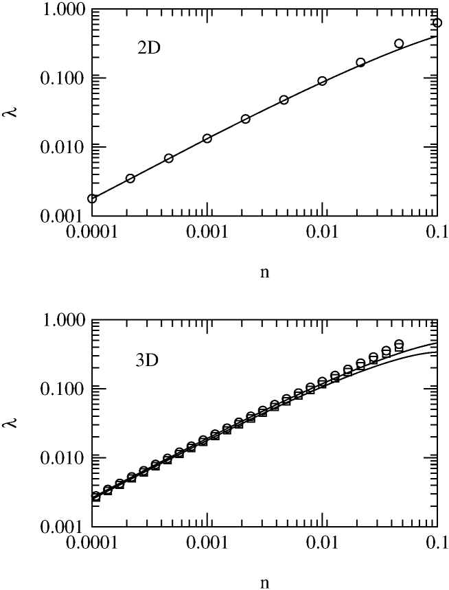
FIG. 7.: A plot of the Lyapunov exponents, in units of $v/a$, for the moving particle in a random, dilute Lorentz gas in two dimensions (top) and three dimensions (bottom), as functions of the density $n$, in units of $a^{-d}$. The solid lines are the results given by kinetic theory, Eq. (125), respectively, Eqs. (126) and (128), and the data points are the numerical results of Dellago and Posch.

B Formal Kinetic Theory for the Low Density Lorentz Gas

The formal theory for the KS entropy of the regular gas is easily applied to the Lorentz gas, which is, of course, considerably simpler. Thus by following the arguments leading to Eq. (19) for the sum of the positive Lyapunov exponents for the regular gas, we find that the KS entropy for the equilibrium Lorentz gas is given by

$$\sum_{\lambda_{i}>0}\lambda_{i}=a^{d-1}\int dx\,d\mbox{\boldmath{$\rho$}}\,d\vec{R}d\hat{\sigma}\Theta(-\vec{v}\cdot\hat{\sigma})|\vec{v}\cdot\hat{\sigma}|\delta(\vec{r}-\vec{R}-a\hat{\sigma})\times$$ (129)

$$\ln|\det\left[{\bf{M}}_{\hat{\sigma}}+2{\bf{Q}}_{\hat{\sigma}}\cdot\mbox{\boldmath{$\rho$}}\right]|{\cal{F}}_{2}(x,\vec{R},\mbox{\boldmath{$\rho$}}).$$ (130)

Here $\vec{R}$ denotes the location of the scatterer with which the moving particle is colliding, and ${\cal{F}}_{2}$ is the pair distribution function for the moving particle to have coordinate, $\vec{r}$, velocity, $\vec{v}$, ROC matrix, $\rho$, while the center of the scatterer is located at $\vec{R}$. At low densities we may assume that the moving particle and the scatterer are uncorrelated, so that the density expansion for ${\cal{F}}_{2}$, immediately before collision would have the form

$${\cal{F}}_{2}(x,\vec{R},\mbox{\boldmath{$\rho$}})=n{\cal{F}}_{1}(x,\mbox{\boldmath{$\rho$}})+\ldots,$$ (131)

where $n$ is the number density of the scatterers and ${\cal{F}}_{1}(x,\mbox{\boldmath{$\rho$}})$ is the equilibrium single particle distribution function for the moving particle.

We may easily construct an extended Lorentz-Boltzmann equation (ELBE) for ${\cal{F}}_{1}$ along the lines used previously for the extended Boltzmann equation in Section III. The ELBE is given by [13, 14]

$$\left[\frac{\partial}{\partial t}+{\cal{L}}_{0}\right]{\cal{F}}_{1}(x,\mbox{\boldmath{$\rho$}})=a^{d-1}\int d{\vec{R}}d\hat{\sigma}\Theta(-\vec{v}\cdot{\hat{\sigma}})|(\vec{v}\cdot\hat{\sigma})\times$$ (132)

$$\left[\delta(\vec{r}-\vec{R}-a\hat{\sigma})\int d\mbox{\boldmath{$\rho$}}^{\prime}\delta(\mbox{\boldmath{$\rho$}}-\mbox{\boldmath{$\rho$}}(\mbox{\boldmath{$\rho$}}^{\prime})){\cal{P}}^{\prime}_{\hat{\sigma}}-\delta(\vec{r}-\vec{R}+a\hat{\sigma})\right]{\cal{F}}_{1}(x,\mbox{\boldmath{$\rho$}}).$$ (133)

Here the operator ${\cal{P}^{\prime}_{\hat{\sigma}}}$ is a substitution operator that replaces velocities, $\vec{v}$ and ROC matrices, $\rho$, by their restitution values, i.e., the values needed before collision to produce the values $\vec{v}$, and $\rho$ after collision with a scatterer with collision vector $\hat{\sigma}$. Also, the free particle streaming operator on the left-hand side of Eq. (133) is given by

$${\cal{L}}_{0}=\vec{v}\cdot\frac{\partial}{\partial\vec{r}}+\sum_{\alpha=1}^{d}\frac{\partial}{\partial\mbox{\boldmath{$\rho$}}_{\alpha\alpha}},$$ (134)

since between collisions, $\vec{r}$ varies as $\vec{r}(0)+t\vec{v}$ and $\rho$ varies as $\mbox{\boldmath{$\rho$}}(0)+t{\bf{1}}$.

Returning for the moment to Eq. (130) for the KS entropy, we see by evaluating the determinant in the integrand on the right side, that not all components of $\rho$ contribute. In fact, only the components of $\rho$ in the plane perpendicular to $\vec{v}$ contribute to $h_{KS}$. Here we will work out the details of the calculation of $h_{KS}$ for the two dimensional case, leaving the details of the three dimensional case to the literature [14]. For $d=2$ we can easily evaluate the determinant in Eq. (130), and find that it is

$$|\det\left[{\bf{M}}_{\hat{\sigma}}+2{\bf{Q}}_{\hat{\sigma}}\cdot\mbox{\boldmath{$\rho$}}\right]|=1+\left(\frac{2v\rho}{a\cos\phi}\right).$$ (135)

Here the scalar $\rho$ is the component of the $\rho$ matrix given by $\rho=\hat{v}_{\perp}\cdot\mbox{\boldmath{$\rho$}}\cdot\hat{v}_{\perp}$, where $\hat{v}_{\perp}$ is a unit vector orthogonal to $\vec{v}$. Moreover, for low densities we can use the approximation $n{\cal{F}}_{1}(x,\mbox{\boldmath{$\rho$}})$ for ${\cal{F}}_{2}$. Then the expression for $h_{KS}$ becomes, at low densities

$$h_{KS}=an\int dx\,d\rho d\hat{\sigma}\Theta(-\vec{v}\cdot\hat{\sigma})|\vec{v}\cdot\hat{\sigma}|\ln\left[1+\left(\frac{2v\rho}{a\cos\phi}\right)\right]{\cal{F}}_{1}(x,\rho),$$ (136)

where $x=\vec{r},\vec{v}$, and we have to determine $F_{1}(x,\rho)$ as the solution of the ELBE where we integrate over all components of $\rho$, except the one diagonal component $\rho$. The ELBE then becomes, in the spatially homogeneous, equilibrium case

$$\frac{\partial}{\partial\rho}{\cal{F}}_{1}(\vec{r},\vec{v},\rho)=nav\int_{-\pi/2}^{\pi/2}d\phi\,\cos\phi\left[\int_{0}^{\infty}d\rho^{\prime}\delta\Bigg{(}\rho-\frac{a\cos\phi}{2v+\frac{a\cos\phi}{v\rho^{\prime}}}\Bigg{)}{\cal{F}}_{1}(\vec{r},\vec{v}^{\prime},\rho^{\prime})-{\cal{F}}_{1}(\vec{r},\vec{v},\rho)\right].$$ (137)

The argument of the $\delta$ function is simply obtained by using the mirror formula given by Eq. (107), but now the unprimed variable is the value after collision, and the primed variable is the value of $\rho$ before collision. A further, and useful simplification results from the observation that $\rho^{\prime}$ is typically of the order of the mean free time between collisions, which, for low density, is much larger than $a/v$. Therefore the delta function can be replaced by

$$\delta\Bigg{(}\rho-\frac{a\cos\phi}{2v+\frac{a\cos\phi}{v\rho^{\prime}}}\Bigg{)}\approx\delta\left(\rho-\frac{a\cos\phi}{2v}\right){}.$$ (138)

In a spatially homogeneous and isotropic equilibrium state, ${\cal{F}}_{1}$ has to be a function of the norm of the velocity vector $|\vec{v}|$ and the radius of curvature $\rho$ only. Using that the magnitude of the velocity, $|\vec{v}|$, always stays the same, we know that there is a solution of the form

$${\cal{F}}_{1}(\vec{r},\vec{v},\rho)=\varphi(\vec{v})\psi(\rho),$$ (139)

with $\varphi(\vec{v})=(2\pi V)^{-1}\delta(|\vec{v}|-v_{0})$ is the normalized equilibrium spatial and velocity distribution function for the moving particle, $v_{0}$ is its constant speed, and $V$ is the volume of the system. Now all we have to do is to determine $\psi(\rho)$. An inspection of Eq. (137), with the approximation, Eq. (138) shows that $\psi(\rho)$ satisfies the equation

$$\frac{\partial\psi(\rho)}{\partial\rho}+2nav\psi(\rho)=0,$$ (140)

for $\rho\geq a/(2v)$, with solution

$$\psi(\rho)=(1/t_{0})e^{-t/t_{0}}\,\,\,\,{\rm for}\,\,\rho\geq a/(2v).$$ (141)

Here $t_{0}$ is the mean free time given by $t_{0}=(2nav)^{-1}$. In the case that $\rho<a/(2v)$, one can easily solve the full equation with the delta function to find

$$\psi(\rho)=(1/t_{0})\left\{1-\left[1-\left(\frac{2v\rho}{a}\right)\right]^{1/2}\right\}\,\,\,{\rm for}\,\,\rho<a/(2v).$$ (142)

Combining these results with Eq. (139) and inserting them in Eq. (136) we recover the result, Eq. (125) for the KS entropy, equivalently the positive Lyapunov exponent, for the low density, equilibrium, random Lorentz gas. A similar, but somewhat more elaborate calculation can be carried out, for the three dimensional case, to obtain exactly the same result as obtained in the informal theory for the KS entropy. To obtain the largest Lyapunov exponent by more formal methods, one has to resort to methods for determining the largest eigenvalue for products of random matrices. This is well described in the literature [14] and we will not pursue this issue further here.

VI Conclusions and Open Problems

In this article we have given a survey of the applications of the kinetic theory of dilute, hard-ball gases to the calculation of quantities that characterize the chaotic behavior of such systems. Results have been obtained for the KS entropy per particle and for the largest Lyapunov exponent of dilute hard-ball systems, as well as for the Lyapunov spectrum for the moving particle in the dilute, random Lorentz gas, with nonoverlapping, fixed, hard-ball scatterers. All of these results are in good to excellent agreement with the results of computer simulations. In the study of the largest Lyapunov exponent, we have developed a very interesting clock model which seems to explain many features of the behavior of this exponent. Moreover, the method for treating the clock model reveals a deep and, perhaps unexpected, connection between the theory of Lyapunov exponents and the theory of hydrodynamic fronts.

We emphasize that the results given here apply to a dilute gas in equilibrium, but nonequilibrium situations have been treated by these methods as well. For example, it is possible to calculate the Lyapunov spectrum for a dilute, random Lorentz gas in a nonequilibrium steady state produced by a thermostatted electric field, at least for small fields, and to obtain results that are in excellent agreement with computer simulations [33, 34, 32]. Calculations are currently underway for the largest Lyapunov exponent for a hard-ball gas, when the gas is subjected to a thermostatted, external force that maintains a steady shear flow in the gas. Furthermore, one can use kinetic theory to calculate the Lyapunov spectrum for trajectories on the fractal repeller for a Lorentz gas with open, absorbing boundaries [13, 35]. Such results are useful for understanding escape-rate methods for relating chaotic quantities for trajectories on a fractal repeller of an open system to the transport properties of the system, as described by Gaspard and Nicolis [9, 10, 36]. These results will eventually be extended to hard-ball gases as well.

Of course, many problems remain to be solved. Here we mention some of the most immediate problems:

1. All of the results described here apply to hard-core systems. That is the particles interact with a potential energy that is either zero, beyond a given separation, or infinite, below that separation. It is worth studying the properties of dilute systems with smoother potential energies for a number of reasons: (a) The results of Rom-Kedar and Turaev [12] suggest that the dynamics of particles with short ranged but smooth potentials may exhibit regions of nonhyperbolic behavior. It is important to know more about these regions and to assess their effect on the overall chaotic behavior of gases interacting with such potentials. (b) We know very little about the chaotic properties of dilute gases interacting with long range forces, such as Maxwell molecules and Coulomb gases.

2. An open problem, even for dilute gases, is to obtain the complete spectrum of Lyapunov exponents for a hard-ball gas. This is a very challenging problem in mathematical physics, and no easy approach is in sight. There is a very tantalizing set of numerical results by Posch and coworkers [37] showing that the smallest nonzero Lyapunov exponents have a hydrodynamic structure, in that the exponents themselves seem to scale as the inverse of the linear size of the system, and that the spatial deviation vectors seem to form collective modes of both transverse and longitudinal types. Eckmann and Gat [38] have proposed an explanation of this hydrodynamic-like behavior of the lowest Lyapunov modes using techniques from the theory of random matrices. It would be useful to understand and to extend their results using kinetic theory methods.

3. The extension of these results to gases at higher densities remains an open, challenging problem. The kinetic theory of dense gases has exposed a number of effects caused by long range dynamical correlations between the particles. Such effects include nonanalytic terms in the density expansion of transport coefficients and long time tail phenomena in time correlation functions, among others [4]. It is of some interest to see the effect of these dynamical correlations on the chaotic properties of the gas, as well. Furthermore, a high density hard-ball system may form a glass, and there would be useful information obtained about the glassy state if one could study the chaotic behavior of the gas through the glass transition.

4. The extension of the clock model to higher density systems can also be expected to reveal new and interesting phenomena connected to the effects of density and other fluctuations in the gas upon the clock speed and related quantities. At present there are some weak numerical indications [39] that the largest Lyapunov exponent might diverge in the limit of large numbers of particles as $\ln N$, where $N$ is the number of particles in the system. It might be possible to confirm or to rule out this possibility by extending the clock model so as to include the effects of fluctuations in the fluid.

5. Lyapunov exponents and KS entropies are not the only properties that characterize chaotic systems. There are many more quantities, such as topological pressures, fractal dimensions, etc., that remain to be explored by the methods outlined here.

6. A subject of considerable interest and activity is the physics of gases that make inelastic collisions, i.e. the physics of granular materials [40]. One would like to know what the chaotic properties of such systems might be, or, more generally, how to define such properties in nonstationary systems.

In conclusion, we have described in this article only the first steps, taken over the last few years, to develop useful methods for the calculations of Lyapunov exponents and KS entropies for the systems of particles that can be treated by kinetic theory. We are particularly delighted that kinetic theory has something to contribute to the field of the chaotic behavior of large systems of particles, and that the ideas of Maxwell and Boltzmann are still having new and fruitful applications.

Acknowledgements: The authors would like to thank Professor Harald A. Posch, Professor Christoph Dellago, and Dr. Arnulf Latz for many helpful conversations, and for collaborations on much of the research described here. here; We are also grateful to Professor Christoph Dellago and Professor Harald A.  Posch for supplying Figs. 1, 2 and 7. H. v. B. and R. v. Z. are supported by FOM, SMC and by the NWO Priority Program Non-Linear Systems, which are financially supported by the “Nederlandse Organisatie voor Wetenschappelijk Onderzoek (NWO)”. J. R. D. would like to thank the National Science Foundation for support under grant PHY-9600428.

REFERENCES

- [1] S. G. Brush, The Kind of Motion We Call Heat : A history of the kinetic theory of gases in the 19th century, Studies in statistical mechanics vol. 6, North-Holland, Amsterdam (1976).
- [2] L. Boltzmann, Lectures on Gas Theory, S. G. Brush, transl., Dover Publications, New York, (1995).
- [3] S. Chapman and T. Cowling, The Mathematical Theory of Non-uniform Gases, third edition, Cambridge University Press, Cambridge (1970).
- [4] J. R. Dorfman, and H. van Beijeren, in Statistical Physics, Part B, B. J. Berne, ed., Plenum Publishing Co., New York, (1977),p.65.
- [5] P. Ehrenfest and T. Ehrenfest, The Conceptual Foundations of the Statistical Approach in Mechanics, Cornell University Press, Ithaca, (1959).
- [6] G. E. Uhlenbeck and G. W. Ford, Lectures in Statistical Mechanics, American mathematical Society, Providence, (1963).
- [7] J. L. Lebowitz, Physica A, 194, 1, (1993).
- [8] V. I. Arnold and A. Avez, Ergodic Problems of Classical Mechanics, W. A. Benjamin, Inc, New York, (1968).
- [9] P. Gaspard,Chaos, Scattering Theory and Statistical Mechanics, Cambridge University Press, Cambridge (1998).
- [10] J. R. Dorfman, An Introduction to Chaos in Non-equilibrium Statistical Mechanics, Cambridge University Press, Cambridge (1999).
- [11] H. van Beijeren, J. R. Dorfman, Ch. Dellago and H. A. Posch, Phys. Rev. E 56, 5272 (1997).
- [12] V. Rom-Kedar and D. Turaev, Physica D 130, 187 (1999).
- [13] H. van Beijeren and J. R. Dorfman, Phys. Rev. Lett. 74, 4412 (1995); Erratum Phys. Rev. Lett. 76, 3238 (1995).
- [14] H. van Beijeren, A. Latz and J. R. Dorfman, Phys. Rev. E 57, 4077 (1998).
- [15] R. van Zon, H. van Beijeren and Ch. Dellago, Phys. Rev. Lett. 80, 2035 (1998).
- [16] R. van Zon, H. van Beijeren, J. R. Dorfman, Kinetic Theory of Dynamical Systems, preprint chao-dyn/9906040 (1999).
- [17] Ch. Dellago, H. A. Posch and W. G. Hoover, Lyapunov instability in a system of hard disks in equilibrium and nonequilibrium steady states, Phys. Rev. E. 53, 1485-1501 (1996).
- [18] Ya. G. Sinai, Russian Math. Surveys 25, 137, (1970) ; Ya. G. Sinai (ed.), Dynamical Systems, World Scientific Publishing (1991).
- [19] E. Ott, Chaos in Dynamical Systems, Cambridge University Press, Cambridge (1993).
- [20] Ja. B. Pesin, Sov. Math. Doklady 17 (1976), 196; Reprinted in R. S. MacKay and J. D. Meiss, Hamiltonian Dynamical Systems (Adam Hilger, Bristol, 1987).
- [21] J. R. Dorfman, A. Latz, and H. van Beijeren, Chaos 8, Issue 2 (1998) 444
- [22] J. R. Dorfman, (to be published).
- [23] H. van Beijeren, H. Kruis, D. Panja and J. R. Dorfman, to be published.
- [24] C. Cercignani, Theory and Application of the Boltzmann Equation, Scottish Academic Press, Edinburgh/London (1975).
- [25] W. van Saarloos, Phys. Rev. A 37, 211 (1988); U. Ebert and W. van Saarloos, Phys. Rev. Lett. 80, 1650 (1998); U. Ebert and W. van Saarloos, Front propagation into unstable states: Universal algebraic convergence towards uniformly translating pulled fronts, Physica D (to appear).
- [26] Ch. Dellago and H. A. Posch, in [27], pp. 68–83 (1997).
- [27] Special issue on the Proceedings of the Euroconference on The Microscopic Approach to Complexity in Non-Equilibrium Molecular Simulations. CECAM at ENS-Lyon, France, 1996, edited by M. Mareschal, Physica (Amsterdam) 240A (1997).
- [28] G. A. Bird, Molecular Gas Dynamics, Clarendon, Oxford (1976).
- [29] E. Brunet and B. Derrida, Phys. Rev. E 56, 2597 (1997).
- [30] A. Lemarchand and B. Nawakowski, J. Chem. Phys. 109, 7028 (1998).
- [31] Ch. Dellago and H. A. Posch, Phys. Rev. E, 52, 2401, (1995).
- [32] Ch. Dellago and H. A. Posch, Phys. Rev. Lett. 78, 211 (1997).
- [33] H. van Beijeren, J. R. Dorfman, E. G. D. Cohen, Ch. Dellago and H. A. Posch, Phys. Rev. Lett. 77, 1974 (1996).
- [34] A. Latz and H. van Beijeren and J. R. Dorfman, Phys. Rev. Lett. 78, 207 (1997).
- [35] H. van Beijeren, A. Latz, and J. R. Dorfman (to be published).
- [36] P. Gaspard and G. Nicolis, Phys. Rev. Lett. 65, 1693, (1990).
- [37] Lj. Milanović, H. A. Posch and Wm. G. Hoover, Mol. Phys. 95, 281 (1998); H. A. Posch and R. Hirschl, Simulation of billiards and hard-body fluids, preprint, (1999).
- [38] J.-P. Eckmann and O. Gat, preprint chao-dyn/9908018 (1999).
- [39] D. J. Searles, D. J. Evans and D. J. Isbister, in [27], pp. 96–104 (1997).
- [40] M. H. Ernst, in “Proceedings of the NATO-ASI on Dynamics: Models and Kinetic Methods for Non-equilibrium Many Body Systems, J. Karkheck (ed.), 1999.”