Indistinguishable multiplier statistics
of
discrete and continuous turbulent cascade models

Abstract

The multiplier statistics of discrete and continuous nonconservative multiplicative cascade models, employed to describe the energy cascade in fully developed turbulence, is investigated. It is found to be indistinguishable due to small-scale resummation and restoration of spatial homogeneity. Only the subclass of positively skewed weight distributions, associated to the cascade generator, qualifies to describe observed unconditional as well as conditional multiplier distributions qualitatively; popular log-Poisson and log-stable weight distributions do not share this property.

I Introduction

The intermittent small-scale dynamics of fully developed turbulence at very large Reynolds numbers is believed to be more or less scale-invariant within the so-called inertial range, the latter being bound by the integral length scale $L$ and the dissipation length scale $\eta\ll L$. Consequently, both experimental [1] and theoretical [2, 3] efforts largely concentrate on scaling exponents, which are deduced from structure functions of the velocity field. However, “scaling exponents are not everything” as they represent for sure the simplest, but at the same time also the most insensitive observables characterising multi-scale processes. Because of this insensitiveness any heroic effort to derive the observed multi-scaling directly from the Navier-Stokes equation [4, 5] remains somewhat incomplete as some physics might have been lost with the applied approximations and assumptions. Also, due to the finiteness of the real-world inertial range and the limited statistical sampling, the experimental procedure to extract multi-scaling is not unequivocal and quoted values for scaling exponents beyond sixth order should not be overemphasised. For these reasons and also in view of the quest for universality in the up-to-now unreachable limit $R_{\lambda}\rightarrow\infty$, additional observables other than scaling exponents are needed.

In order to explain this philosophy, “scaling exponents are not everything”, in more detail, we discuss heuristic multiplicative cascade processes and show that with a clever subclass of additional observables more can be learned about the intrinsic cascade dynamics than only from scaling exponents. Following Richardsons historic metaphor of large eddies decaying into successively smaller and smaller eddies, a multiplicative cascade process phenomenologically describes the turbulent redistribution of energy flux from large to small scales and is able to reproduce the observed scaling exponents of the surrogate energy dissipation field [3, 6], which are related to those of the velocity structure functions by the Refined Similarity Hypothesis [7]. Originally intended to directly access the multiplicative weight distribution associated to the energy cascade generator distributions of so-called multipliers or break-up coefficients [8] have been extracted from very large Taylor-scale based Reynolds number atmospheric boundary layer and wind tunnel flows recently [9, 10, 11]; see also Ref. [12]. It was found that within the upper part $0\ll l<L$ of the inertial range these multiplier distributions do in fact become scale-independent. However, they do depend on the relative position of parent and daughter domain; this non-homogeneity of the breakup leaves a subsequent extraction of scaling exponents inconsistent [13] and indicates the presence of correlations between successive multipliers, as has been confirmed by studying multiplier distributions conditioned on the value of the (scale-) previous multiplier [10, 11]. The observed correlations appear to be in conflict with the simple multiplicative cascade models, where the cascade generator is assumed to be identical and independent at each breakup. As has been convincingly demonstrated in Refs. [14, 15] this apparent conflict can be resolved: introducing non-conservative cascade generators with a positively skewed weight distribution and restoring Euclidean homogeneity of the ultrametric cascade models, the multiplier distributions resulting from a discrete binary multiplicative cascade become a scale-independent fix-point due to small-scale resummation and are in good qualitative agreement with the experimentally deduced distributions, including all observed correlation effects.

Originally not anticipated, these multiplier distributions represent one of those wanted clever subclasses of additional observables, from which more can be learned about the relevance of cascade processes in turbulence and about the intrinsic cascade dynamics than only from scaling exponents. The experimental analysis [10, 11] reveals that unconditional multiplier distributions are observed to be scale-independent within the range $500\eta\leq l\leq L/2$. In view of the findings of Ref. [15] we call this the visible cascade range. Since due to small-scale resummation it takes about three binary scale steps for the multiplier distributions to converge to the scale-independent fix-point the lowest part of the true cascade range $\eta^{*}\approx 500\eta/2^{3}\approx 60\eta\leq l\leq L$ is not visible. A further conclusion from this line of reasoning would be that below $\eta^{*}$ dissipation dynamics sets in and modifies the scale-independent cascade dynamics. Besides this interpretation about the scope of cascade processes in turbulence, also more details about the intrinsic cascade dynamics can be learned from multiplier distributions [14, 15]. Not every weight distribution, associated to a binary cascade generator and reproducing observed scaling exponents within experimental error bars, qualifies to yield the correct distributions of multipliers and their correlations. It has to come with a positive skewness. Weight distributions of log-normal or certain asymmetric binomial type share this property, whereas, for example, a log-Poisson weight distribution [16] does not.

All those conclusions have been drawn from binary discrete multiplicative cascade processes in connection with base-two ($\lambda=2$) multiplier distributions. Multiplier distributions referring to other scale steps have not been looked at. In this respect it is of interest to find out whether the latter do again reveal a scale-independent fix-point behaviour with additional correlations or whether they are simply artefacts of the binary discrete cascade model implementation. Not only this aspect is of relevance to find answers, the impact of cascade model implementations with scale steps other than $\lambda^{\prime}=2$, i.e. $\lambda^{\prime}>2$ or $\lambda^{\prime}\rightarrow 1$, has to be studied for the multiplier phenomenology: do multiplier distributions resulting from different model implementations differ or not? Put in other words: are different cascade model implementations distinguishable or indistinguishable on the level of multiplier observables? – Theoretically the scale step $\lambda^{\prime}$ associated to the cascade generator is not fixed. Due to the present lack of a derivation of cascade models from the Navier-Stokes equation, no specific choice is favoured for $\lambda^{\prime}$, except for personal taste. Only if the last question can be answered with yes, we can consider multiplier distributions as a clever subclass of additional observables.

The organisation of the paper is as follows: In Sect. II we sketch the implementation of general multiplicative cascade processes and briefly summarize previous work on ($\lambda=2$)-multiplier distributions resulting from a discrete ($\lambda^{\prime}=2$) model implementation. Sect. III concentrates on discrete ($\lambda^{\prime}\geq 2$) implementations of multiplicative cascade processes and presents multiplier distributions referring to scale steps $\lambda\neq 2$. A quasicontinuous implementation of random multiplicative cascade models is used in Sect. IV to study respective multiplier distributions referring to various scale steps. So-called log-stable weight distributions [17, 18] are considered in Sect. V and, although leading to correct scaling exponents [19, 20], shown not to reproduce the observed multiplier distributions. Several conclusions are presented in Sect. VI, the most important being that it does not matter how multiplicative cascade models are implemented (discrete or continuous), since the multiplier observables are indistinguishable.

II Implementation of discrete and continuous multiplicative cascade models

A Implementation

The following one-dimensional implementation of multiplicative cascade processes is designed to model the energy cascade from large ($L$) to small ($\eta^{*}$) length scales:

The initial energy flux density field at the integral scale $L$ is set equal to $\varepsilon(x,L)=1$ without any loss of generality. For an intermediate length scale $\eta^{*}\leq l<L$ we introduce a so-called weight field

$$q(x,l)=\sum_{k=-\infty}^{\infty}q_{k}(l)\Theta(x-kl,l)\;,$$ (1)

where the index function

$$\Theta(x,l)=\left\{\begin{array}[]{ll}1&\qquad(0\leq x<l)\\ 0&\qquad(x<0,\,x\geq l)\end{array}\right.$$ (2)

represents a subdomain of length $l$. Each random weight $q_{k}(l)$ is independently drawn from a scale-independent probability distribution $p(q)$ with mean $\langle q\rangle=1$. The energy density field

$$\varepsilon(x,\eta^{*})=\left(\prod_{i=1}^{n}q(x,l_{i})\right)\varepsilon(x,L)$$ (3)

at the smallest scale $\eta^{*}$ is then constructed as a multiplication of weight fields belonging to a hierarchy of different intermediate length scales $l_{i}=L/(\lambda^{\prime})^{i}$, where $(\lambda^{\prime})^{n}=L/\eta^{*}$.

Let us discuss the special case for $\lambda^{\prime}=2$, so that it is sufficient to consider the fields only in the domain $0\leq x<L$. The implementation (3) can then be understood in terms of a binary cascade generator: The energy density $\varepsilon(l)$ of a domain of length $l$ is redistributed onto a left and right subdomain of length $l/2$ with energy densities $\varepsilon_{L}(l/2)=q_{L}\varepsilon(l)$ and $\varepsilon_{R}(l/2)=q_{R}\varepsilon(l)$, where the random weights are drawn from the splitting function

$$p(q_{L},q_{R})=p(q_{L})p(q_{R})\;.$$ (4)

The successive application of this cascade generator from the large scale $L$ down to the small scale $\eta^{*}$ leads to the field (3). – The splitting function (4) is not in its most general form as it does not need to factorise. However, it has been noted in Ref. [15], that because fully developed turbulence is a $3+1$ dimensional process, the observational reduction of a more-dimensional multiplicative cascade process to one dimension leads to a splitting function which factorises almost completely.

B Observables

The standard observable of multiplicative cascade processes are scaling exponents representing the intermittency corrections. They are deduced from a scale-invariant moment analysis of the synergetic field (3); a naive derivation gives

$$\left\langle\varepsilon(x,l_{m})^{\nu}\right\rangle=\left\langle q(x,l)^{\nu}\right\rangle^{m}=\left(\frac{L}{l_{m}}\right)^{\tau(\nu)}=(\lambda^{\prime})^{m\tau(\nu)}$$ (5)

with scaling exponents

$$\tau(\nu)=\frac{\ln\langle q^{\nu}\rangle}{\ln\lambda^{\prime}}\;,$$ (6)

where the independence of the $m$ weights $q(x,l_{1})$, …, $q(x,l_{m})$ has been exploited. This deduction is not in full accordance with the analysis of experimentally measured fields; those are recorded at the finest resolution scale $\eta<\eta^{*}$, then averaged over larger length scales $l$,

$$\overline{\varepsilon}(x,l)=\frac{1}{l}\int_{x-l/2}^{x+l/2}\varepsilon(x^{\prime},\eta)dx^{\prime}\;,$$ (7)

and are not identical to the model field evolved from scales $L$ to $l$ [15, 17], i.e.

$$\overline{\varepsilon}(x,l)\neq\varepsilon(x,l)\;.$$ (8)

The scale dependence of moments $\langle\overline{\varepsilon}(x,l)^{\nu}\rangle$ of the backward field are different from (5) and do not show rigorous scaling at the very small scales [21]. Only in the large-scale asymptotic scaling exponents can be extracted unambiguously and coincide with the expression (6).

Originally proposed in Ref. [8] and applied in Refs. [9, 10, 11, 12] the method of random multipliers (or break-up coefficients) aims at directly accessing scaling exponents via respective distributions of the former. In its most general form multipliers are defined as

$$M(x,l;\lambda,\Delta)=\frac{\overline{\varepsilon}(x^{\prime},\frac{l}{\lambda})}{\lambda\overline{\varepsilon}(x,l)}\;,$$ (9)

where $\overline{\varepsilon}(x^{\prime},\frac{l}{\lambda})$ represents the averaged energy density over an offspring interval of length $l/\lambda$ and with its centre shifted by $x^{\prime}-x=(1-\lambda^{-1})l\Delta$ with respect to the parent interval. We distinguish three special cases for the shift parameter $\Delta$: for $\Delta=0$, $\pm 1/2$ we call $M(x,l;\lambda,\Delta)$ centred, right- and left-sided, respectively. – For very large Reynolds number turbulent flows it has been found experimentally [9, 10, 11] that the unconditional multiplier distributions $p(M(l;\lambda,\Delta))$, which are sampled over $x$, do not depend on the scale $l$ within the regime $\eta\ll l\leq L/2$. However, a dependence on the shift parameter $\Delta$ was noticed; this “nonhomogeneity of the breakup” obscures the relationship between multiplier and weight distribution and the once intended extraction of scaling exponents [13]. Actually the $\Delta$-dependence hints to the existence of correlations between successive multipliers. These correlations have been observed in conditional multiplier distributions $p(M(x^{\prime},l/\lambda;\lambda,\Delta)|M(x,l;\lambda,\Delta))$ with left/right-sided ($\Delta=\pm 1/2$) [10] and centred ($\Delta=0$) [11] shift parameter, respectively, and with the emphasis on base-two ($\lambda=2$) scale steps.

These latest findings appear to contradict the simple multiplicative cascade processes with independent breakups. However, this statement is not true! The studies in Refs. [14, 15] with nonconservative binary ($\lambda^{\prime}=2$) random multiplicative cascade models have given a new interpretation to multiplier distributions: unconditional multiplier distributions represent a scale-independent fix-point due to small-scale resummation; the “nonhomogeneity of the breakup” is also naturally explained along this line. Once the sampling of multipliers is allowed over all and not only dyadic positions the correct multiplier correlations have been obtained from positively skewed weight distributions; for example, a log-normal weight distribution does qualify whereas a log-Poisson distribution does not qualify. These results show that multiplier distributions do reveal more information about the underlying weight distribution than might be extracted from approximate scaling exponents.

III Multiplier statistics of discrete multiplicative cascade models

A Discrete multiplicative cascade models with binary splittings

For discrete multiplicative cascade models with binary splittings the scale step entering into the construction of the energy density field (3) is set equal to $\lambda^{\prime}=2$. Furthermore, we choose $n=10$. The length of the field configuration is set equal to $0\leq x\leq 10^{5}L$, mimicking a long time series. As weight distribution we choose the binomial distribution

$$p(q)=\frac{\alpha_{2}}{\alpha_{1}+\alpha_{2}}\delta\left(1-(1-\alpha_{1})\right)+\frac{\alpha_{1}}{\alpha_{1}+\alpha_{2}}\delta\left(1-(1+\alpha_{2})\right)$$ (10)

with parameters $\alpha_{1}=0.3$, $\alpha_{2}=0.65$; this choice has the correct skewness $S_{3}=\langle(q-\langle q\rangle)^{3}\rangle/(\langle(q-\langle q\rangle)^{2}\rangle)^{3/2}=(\alpha_{2}-\alpha_{1})/\sqrt{\alpha_{1}\alpha_{2}}>0$ in order to reproduce conditional base-two multiplier distributions [14]. Other, non-binomial weight distributions, such as of log-normal or Pearson-III type, are also able to provide a positive skewness and lead to more or less identical base-two multiplier distributions [15], all being in qualitative accordance with experimental findings [10, 11]. Also multiplier distributions different from base-two do not distinguish the aforementioned weight distributions. Hence, we will only show results for the weight distribution (10).

Due to small-scale resummation [15] the base-two multiplier distributions are scale-invariant in the regime $8\eta^{*}\leq l\leq L/2$; for $\eta^{*}\leq l\leq 8\eta^{*}$ the distributions converge to the scale-independent fix-point and for scales very close to the integral length scale deviations from scale-invariance set in because of the finiteness of $L$. Figure 1(a2) shows simulation results for left-sided multiplier distributions ($\Delta=-0.5$) at scale $l=L/8$: the unconditional multiplier distribution $p(M(l;2,-0.5))$ comes close to a Beta-distribution parametrisation

$$p(M)=\frac{\Gamma(\beta_{1}+\beta_{2})}{\Gamma(\beta_{1})\Gamma(\beta_{2})}M^{\beta_{1}-1}(1-M)^{\beta_{2}-1}$$ (11)

with $\beta_{1}=\beta_{2}=3.2$, which has been extracted from very large Reynolds number atmospheric boundary layer turbulence [10]. Once conditioned on the respective parent multiplier, correlations are observed: the distribution $p(M(l;2,-0.5)|0.5\leq M(2l;2,-0.5)\leq 1)$ with a large parent multiplier becomes broader than the unconditional distribution and its average is shifted to a value larger than $1/2$. The opposite holds for the conditional distribution $p(M(l;2,-0.5)|0\leq M(2l;2,-0.5)\leq 0.5)$ with a small parent multiplier; it is more narrow than the unconditional distribution and its average is shifted to a value smaller than $1/2$. The positive correlation between left-sided daughter and left-sided parent multiplier is a consequence of the homogeneous sampling of multipliers over all $x$-positions, which is not restricted to dyadic cascade positions. Respective multiplier distributions of right/right combinations are identical to these left/left combinations. A negative correlation between daughter and parent multipliers is revealed for identical left/right and right/left combinations; their respective distributions are mirror images of those for left/left and right/right combinations, i.e. $p(M(l;2,0.5)|\underline{M}\leq M(2l;2,-0.5)\leq\overline{M})=p(1-M(l;2,-0.5)|\underline{M}\leq M(2l;2,-0.5)\leq\overline{M})$. This explains that conditional distributions, which are averaged over all four daughter/parent combinations, are again symmetric around $M(\lambda=2)=1/2$; these distributions have been shown in Refs. [10, 14, 15].

Left-sided multiplier distributions for scale steps different from $\lambda=2$ are shown in Figs. 1(a1+a3). For $\lambda=4$ the unconditional multiplier distribution converges to a fix-point for $\eta^{*}\ll l\leq L/2$; its maximum is shifted towards smaller values since its average amounts to $\langle M(\lambda=4)\rangle=1/\lambda=0.25$. A conditioning on a left-sided parent multiplier again reveals correlations between successive multipliers: the distribution $p(M(l;4,-0.5)|0.25\leq M(4l;4,-0.5)\leq 1)$ is broader than the unconditional one, whereas $p(M(l;4,-0.5)|0\leq M(4l;4,-0.5)\leq 0.25)$ is more narrow. – Also multiplier distributions of base step close to one, e.g. $\lambda=2^{1/4}$, show fix-point behaviour in the regime $\eta^{*}\ll l\leq L/2$. In view of the discrete ($\lambda^{\prime}=2$)-steps used in the cascade evolution this result appears unexpected on first sight, but again it is small-scale resummation, which explains this result on second thought. The unconditional left-sided distribution comes with an average of $\langle M(\lambda=2^{1/4})\rangle=1/\lambda=0.84$ close to one. The respective conditional distributions $p(M(l;2^{1/4},-0.5)|0\leq M(2^{1/4}l;2^{1/4},-0.5)\leq 0.84)$ and $p(M(l;2^{1/4},-0.5)|0.84\leq M(2^{1/4}l;2^{1/4},-0.5)\leq 1)$ both deviate from the unconditional distribution, but contrary to the $\lambda=2$ and $\lambda=4$ cases, the former has now become broader whereas the latter turns out to be more narrow. Closer inspection reveals that this tendency has been reversed at around $\lambda\approx 1.75$.

Centred multiplier distributions for scale steps $\lambda=4$, $2$ and $2^{1/4}$ do qualitatively show the same behaviour as the respective left-sided multiplier distributions depicted in Figs. 1(a1)-(a3). All centred distributions are more narrow than their respective left-sided counterparts, reflecting again the “nonhomogeneity of the breakup”. This is also illuminated in Fig. 2, where the $\lambda$-dependence of the two exponents $\beta_{1}$ and $\beta_{2}$ of the Beta-distribution (11), fitted to the respective unconditional left-sided and centred multiplier distributions, are shown. Since according to (11) we have $\langle M\rangle=\beta_{1}/(\beta_{1}+\beta_{2})$, the two exponents are related by setting $\langle M\rangle=\lambda^{-1}$.

Conditional multiplier distributions of base step different from $\lambda=2$ have not been looked at in Refs. [10, 11]. Hence, we consider our respective simulation results as predictions.

B Discrete multiplicative cascade models with triple and quadruple splittings

Most often discrete multiplicative cascade models are chosen with scale steps $\lambda^{\prime}=2$. Now we will consider $\lambda^{\prime}=3$ and $\lambda^{\prime}=4$ and investigate the resulting multiplier distributions. Within the implementation (1)-(3) the parameters are chosen as $n=7$ and $0\leq x\leq 10^{5}L$. Again for demonstration, the binomial weight distribution (10) is picked with new parameters $\alpha_{1}=0.37$, $\alpha_{2}=0.8$ for $\lambda^{\prime}=3$ and $\alpha_{1}=0.42$, $\alpha_{2}=0.92$ for $\lambda^{\prime}=4$. According to the expression (6) the two parameter settings yield an acceptable intermittency exponent $\tau(2)=0.236$, but actually have been fitted to reproduce the experimentally deduced unconditional left-sided base-two ($\lambda=2$) multiplier distribution (11) with $\beta_{1}=\beta_{2}=3.2$ in the fix-point scale regime $\eta^{*}\ll l<L/2$. For both cases the resulting unconditional and conditional left-sided fix-point multiplier distributions of bases $\lambda=4$, $\lambda=2$ and $\lambda=2^{1/4}$ are almost indistinguishable from the respective distributions shown in Figs. 1(a1)-(a3) for the binary discrete multiplicative cascade implementation with $\lambda^{\prime}=2$. The same holds for centred multiplier distributions.

For parameter choices $\alpha_{1}$, $\alpha_{2}$, resulting in a negative skewness of the binomial weight distribution, the shape of the resulting unconditional left-sided fix-point multiplier distribution turns out to deviate from the symmetric Beta-distribution parametrisation to some small, but noticeable extend. Moreover, the correct effects observed in the conditional multiplier distributions can not be reproduced. – On the contrary, well adjusted log-normal weight distributions come again with the correct positive skewness and almost identically reproduce all unconditional and conditional multiplier distributions derived from the good binomial weight parametrisations.

IV Multiplier statistics of continuous multiplicative cascade models

A Continuous multiplicative cascade models

A discrete implementation of random multiplicative cascade processes is often opposed by the question ”why discrete?”. It is true that a continuous implementation leads to nicer mathematics in terms of log-infinite divisible and log-stable distributions [17, 18, 19, 20, 22, 23], but since the relationship of the random multiplicative cascade processes to the Navier-Stokes equation is unclear for the moment we prefer to consider discrete and continuous versions on an equal footing. – As far as the numerical implementation is concerned a continuous random multiplicative cascade process will always be quasi-continuous. Hence, Eqs. (1)-(3) do apply with a quasi-continuous scale step $\lambda^{\prime}$ close to one; we choose $\lambda^{\prime}=2^{1/8}$, which compared to a binary cascade corresponds to an eightfold scale-densification. Other parameters are set equal to $n=80$ and $0\leq x\leq 10^{5}L$. Due to scale-densification the binomial weight distribution (10) now comes with rescaled parameters. The setting $\alpha_{1}=0.1$, $\alpha_{2}=0.22$ comes from a fit of the resulting unconditional left-sided base-two multiplier distribution to the expression (11) with $\beta_{1}=\beta_{2}=3.2$; see Fig. 1(b2). Using Eq. (6) it also yields an intermittency exponent of $\tau(2)=0.25$.

Because of small-scale resummation all multiplier distributions become again scale-independent fix-points in the range $\eta^{*}\ll l\leq L/2$; to be more concrete, the simulations reveal a lower bound of approximately $8\eta^{*}$. The unconditional left-sided multiplier distributions of base-scale $\lambda=4$, $2$ and $2^{1/4}$, which are shown in Figs. 1(b1)-(b3), are hard to distinguish from those obtained from a scale-discrete cascade implementation, which are illustrated in Figs. 1(a1)-(a3). A similar statement can be made not only about the respective left-sided conditional distributions, but also for all unconditional and conditional centred multiplier distributions. This finding demonstrates that multiplier distributions in the fix-point regime do not distinguish discrete and continuous versions of random multiplicative cascade processes; again, the reason for this is small-scale resummation.

Other suitable parameter settings of the binomial weight distribution quite easily reproduce all unconditional multiplier distributions shown so far. Even with a different-signed skewness, as for example with $\alpha_{1}=0.195$, $\alpha_{2}=0.1$, the correlation effects observed in the resulting conditional multiplier distributions go in the right direction, but are reduced by a factor of about $2$ in magnitude. – Another interesting parameter setting is $\alpha_{1}=1-\gamma_{1}(\lambda^{\prime})^{\gamma_{2}}$, $\alpha_{2}=(\lambda^{\prime})^{\gamma_{2}}-1$. In the limit $\lambda^{\prime}\rightarrow 1^{+}$ with $\gamma_{1}=\gamma_{2}=2/3$ the weight distribution comes with a large negative skewness $S_{3}=-1/\sqrt{2(\lambda^{\prime}-1)}$ and leads to the infinite divisible log-Poisson cascade model of Refs. [16, 23]. All unconditional multiplier distributions shown so far are again reproduced, but only very weak correlation effects are observed in the resulting conditional multiplier distributions. This demonstrates that although the log-Poisson cascade model is capable to reproduce scaling exponents with no doubt, it fails to describe the correlation systematics of multiplier distributions.

These findings suggest that in order to reproduce unconditional as well as correct conditional multiplier distributions the weight distribution has to possess a positive skewness, irrespective of the chosen scale-step-$\lambda^{\prime}$ implementation of the underlying multiplicative cascade process. For the binomial weight distribution (10) we note that for the qualitatively best parameter choices, i.e. ($\alpha_{1}$, $\alpha_{2}$) $=$ ($0.1$, $0.22$), ($0.3$, $0.65$), ($0.37$, $0.8$), ($0.42$, $0.92$) for $\lambda^{\prime}=2^{1/8}$, $2$, $3$, $4$, respectively, the resulting skewness almost coincides at a value around $S_{3}\approx 0.8$. Here a more quantitative analysis, driven by very large Reynolds number data, would certainly deserve future consideration. – Multiplier distributions resulting from a meticulously tuned log-normal weight distribution

$$p(q)=\frac{1}{\sqrt{2\pi}\sigma q}\exp\left(-\frac{1}{2\sigma^{2}}\left(\ln q+\frac{\sigma^{2}}{2}\right)^{2}\right)$$ (12)

are also practically indistinguishable from the results shown in Fig. 1. Qualitative best parameters for the implementations with $\lambda^{\prime}=2^{1/8}$, $2$, $3$, $4$ are $\sigma=0.15$, $0.42$, $0.55$, $0.60$, respectively, reflecting an approximate, but obvious log-normal dependence $\sigma\sim\sqrt{\log_{2}\lambda^{\prime}}$. Contrary to the case of the binomial weight distribution, the skewness of the respective log-normal distributions is not identical; it increases with increasing $\lambda^{\prime}$ and stays positive for all four cases.

B Continuous-turned-discrete multiplicative cascade models

The multiplier statistics of continuously implemented multiplicative cascade processes appears to be indistinguishable from their discrete counterparts. This poses the question to what degree a continuous multiplicative cascade process might be described by an effective discrete multiplicative cascade process.

For the translation of a continuous into a discrete multiplicative cascade process it is important to deal with the forward field. In analogy to Eq. (3) the energy density field is evolved from integral down to the intermediate binary target length scales $l$ and $l/2$, respectively, i.e.

$$\varepsilon(x,l) = \left(\prod_{i=1}^{n_{l}}q(x,l_{i})\right)\varepsilon(x,L)\;,$$ (13)

$$\varepsilon(x,\frac{l}{2}) = \left(\prod_{i=n_{l}+1}^{n_{l}+d}q(x,l_{i})\right)\varepsilon(x,l)$$ (14)

with $2\eta^{*}\leq l\leq L$, $(\lambda^{\prime})^{n_{l}}=L/l$ and the scale-densification $d=\ln 2/\ln\lambda^{\prime}$. We restrict the $x$-regime to $0\leq x\leq 10^{5}L$. The averaging

$$\underline{\varepsilon}(x,l) = \frac{1}{l}\int_{x}^{x+l}\varepsilon(x^{\prime},l)dx^{\prime}\;,$$ (15)

$$\underline{\varepsilon}_{L}(x,\frac{l}{2}) = \frac{2}{l}\int_{x}^{x+l/2}\varepsilon(x^{\prime},l/2)dx^{\prime}\;,$$ (16)

$$\underline{\varepsilon}_{R}(x,\frac{l}{2}) = \frac{2}{l}\int_{x+l/2}^{x+l}\varepsilon(x^{\prime},l/2)dx^{\prime}$$ (17)

with discrete positions $x=kl$, $0\leq k<10^{5}L/l$ is principally different from the backward averaging of Eq. (7) and leads to the binary weights

$$q_{L} = \frac{\underline{\varepsilon}_{L}(x,\frac{l}{2})}{\underline{\varepsilon}(x,l)}\;,$$ (18)

$$q_{R} = \frac{\underline{\varepsilon}_{R}(x,\frac{l}{2})}{\underline{\varepsilon}(x,l)}\;.$$ (19)

Sampling over all discrete positions leads to a binary splitting function $p_{\rm eff}(q_{L},q_{R})$, which still might depend on the scale $l$.

For the numerical simulations of a concrete quasi-continuous cascade process again an eightfold scale-densification ($d=8$) has been chosen together with the binomial weight distribution (10) with parameters $\alpha_{1}=0.1$, $\alpha_{2}=0.22$. The effective binary splitting function $p_{\rm eff}(q_{L},q_{R})$ with effective weights (18) is illustrated in Fig. 3a for an intermediate length scale. For $\eta^{*}\leq l\leq L/2$ it is practically scale-independent; only at the very large scales a weak scale-dependence is observed. The projected weight distributions $p_{\rm eff}(q_{L})=\int p_{\rm eff}(q_{L},q_{R})dq_{R}$ and $p_{\rm eff}(q_{R})=\int p_{\rm eff}(q_{L},q_{R})dq_{L}$ are identical and come close to a log-normal distribution with a positive skewness. Observe in Fig. 3b that the projected weight distribution is not simply a $d$-fold convolution of the binomial weight distribution (10); the modification is a result of the multivariate implementation (1) of the weight fields. Note also, that the effective splitting function does not strictly factorise; a small correlation between the two effective weights $q_{L}$ and $q_{R}$ exists as the relative entropy $S_{\rm rel}=-\int dq_{L}dq_{R}p_{\rm eff}(q_{L},q_{R})\ln(p_{\rm eff}(q_{L},q_{R})/p_{\rm eff}(q_{L})p_{\rm eff}(q_{R}))\approx-0.1<0$ turns out to be negative.

So far the continously implemented multiplicative cascade process has been directly translated into a ($\lambda^{\prime}=2$)-discrete multiplicative cascade process with an effective splitting function $p_{\rm eff}(q_{L},q_{R})$. For consistency we still have to check, whether this effective ($\lambda^{\prime}=2$)-discrete multiplicative cascade process leads to identical results for the multiplier statistics. The discrete implementation (1)-(3) with $\lambda^{\prime}=2$ and $p_{\rm eff}(q_{L},q_{R})$ instead of Eq. (4) leads to the multiplier distributions shown in Figs. 1(c1)-(c3). Qualitatively there is no difference to the distributions illustrated in Figs. 1(a1)-(a3), (b1)-(b3) and quantitative differences remain very small.

V No room for log-stability

In this Section we want to demonstrate again, that “scaling exponents is not everything”. In view of renormalisation theory so-called log-stable distributions represent mathematically very attractive parametrisations for the weight distribution $p(q)$, leading its way to the denotation “universal multifractals” [18]. In connection with the energy cascade in fully developed turbulence they have already been discussed in Refs. [19, 20], where the expression

$$\tau(\nu)=\tau(2)\frac{n^{\alpha}-n}{2^{\alpha}-2}$$ (20)

has been derived for the scaling exponents (6). With an intermittency exponent of $\tau(2)=0.22$ and a stable index of $\alpha\approx 1.6$ the experimentally deduced scaling exponents [24] are reproduced remarkably well. Focusing on multiplier distributions, we will now reveal limitations of log-stable weight distributions.

Concentrating first on a discrete implementation of multiplicative cascade processes, where according to (1)-(3) the parameters are set as $\lambda^{\prime}=2$, $n=10$ and $0\leq x\leq 10^{5}L$, the associated log-stable weight distribution $p(q)$ is constructed by noting that $-\ln q\sim S_{\alpha}(\sigma,\beta,\mu)$ is distributed according to a stable distribution [25]. The skewness parameter has to be set equal to $\beta=1$ and the scale and shift parameters $\sigma$ and $\mu$ are fixed by the scaling exponents $\tau(1)=0$ and $\tau(2)=0.22$. For various stable parameters $0<\alpha\leq 2$ the respective log-stable weight distributions are illustrated in Fig. 4a. Depending on $\alpha$ these distributions possess different asymmetries with respect to the average $\langle q\rangle=1$; in fact the skewness $S_{3}=\langle(q-\langle q\rangle)^{3}\rangle/\langle(q-\langle q\rangle)^{2}\rangle^{1.5}$, which should neither be confused with the skewness parameter $\beta$ nor with the notation $S_{\alpha}$ of the stable distributions, amounts to $S_{3}=-0.43$, $0.06$, $0.63$, $1.28$ for $\alpha=1.25$, $1.5$, $1.75$, $2.00$. If a correct skewness is really a good criterion to reproduce unconditional as well as conditional multiplier distributions, then according to what we now know from the previous Sections it should be around $S_{3}\approx 1$ for $\lambda^{\prime}=2$. This would limit the stable index $\alpha$ to a regime close to $2$.

The unconditional left-sided base-two multiplier distributions resulting from the log-stable weight distributions with a given index $\alpha$ are again scale-independent in the scale range $8\eta^{*}\leq l\leq L/2$ and are illustrated in Fig. 4b. Since the log-stable weight distributions have already been fitted to the scaling exponent $\tau(2)$, there is no further free parameter left to adjust to the observed unconditional left-sided multiplier distribution (11) with $\beta_{1}=\beta_{2}=3.2$. For $\alpha\geq 1.5$ the agreement is acceptable. Notice especially the extra contributions at $M=0$ and $M=1$ for small values of $\alpha$. This is a consequence of the algebraic tails of the stable-distributions, which lead to excess contributions at $q\approx 0$ in the corresponding weight distributions; consult again Fig. 4a.

The conditional multiplier distributions $p(M(l;2,\pm 0.5)|\underline{M}\leq M(2l;2,\pm 0.5)\leq\overline{M})$ are also shown in Fig. 4b, where over all four possible left/right-sided daughter/parent multiplier combinations has been averaged. For $\alpha=2$ a conditioning on a small parent multiplier, i.e. $(\underline{M},\overline{M})=(0,0.5)$, leads to a distribution more narrow than the unconditional distribution and a conditioning on a large parent multiplier, i.e. $(\underline{M},\overline{M})=(0.5,1)$, leads to a broader distribution. This is in qualitative agreement with the experimental findings of Ref. [10]. For $\alpha=1.75$ this tendency has almost vanished, for $\alpha=1.5$ it has vanished and for $\alpha=1.25$ it has even been reversed. A very similar behaviour is observed in the conditional centred base-two multiplier distributions, which are depicted in Fig. 4c; only for $\alpha$ very close to 2 they are in qualitative agreement with the experimental findings of Ref. [11]. This outcome also confirms our conjecture from above that a correct positive skewness is needed for the weight distribution in order to reproduce the multiplier distributions.

A quasi-continuous implementation of multiplicative cascade processes with log-stable weight distributions leads to multiplier distributions, which are identical to those shown in Figs. 4b+c for the discrete implementation. Hence, we arrive at the conclusion that although scaling exponents are well fitted by log-stable weight distributions with index $\alpha\approx 1.5$ [19, 20] the observed systematics of the multiplier distributions rules out such a stable index value. The log-normal limit $\alpha\approx 2$ reproduces the multiplier distributions much better.

VI Conclusions

Discrete and continuous implementations of geometric multiplicative cascade processes are both able to model multifractal characteristics observed in the surrogate energy dissipation field of fully developed turbulence. Since their relation to the Navier-Stokes equation remains unclear neither form of implementation is principally favoured over the other. Although perhaps somewhat unexpected, this indistinguishability remains once a specific class of observables, going beyond scaling exponents, is employed: multiplier distributions referring to various scale-steps, discrete or quasi-continuous, do not care whether they result from discrete or continuous versions of nonconservative multiplicative cascade processes. The reason for this is that the multivariate model implementation implies a small-scale resummation leading to scale-independent fix-point distributions. From an analysis point of view a discrete or continuous multiplicative cascade process with no correlations between the various branchings appears as a continuous multiplicative cascade process with correlations.

There is more to learn from these fix-point multiplier distributions: not every weight distribution associated to the cascade generator, which matches scaling exponents within experimental error bars, qualifies to reproduce the observed multiplier correlations. The weight distribution has to possess a positive skewness. For example, so-called log-stable distributions with a stable index not close to $\alpha=2$ do not share this property and are unable to reproduce the observed conditional multiplier distributions. – This leaves us with a speculation: The original idea to directly access scaling exponents via unconditional multiplier distributions does not work due to the observed correlations between multipliers. However, these correlations help to restrict the broad class of cascade weight distributions, which all reproduce the observed lowest-order scaling exponents, to those having a positive skewness. A further restriction of this subclass appears to be possible with yet additional observables to be derived from the full analytic solution of the multivariate cascade characteristic function [26]. Then, by directly accessing the cascade weight distribution, it is tempting to study its dependence on the Reynolds number and on the flow configuration, and, thus, to check for universality.

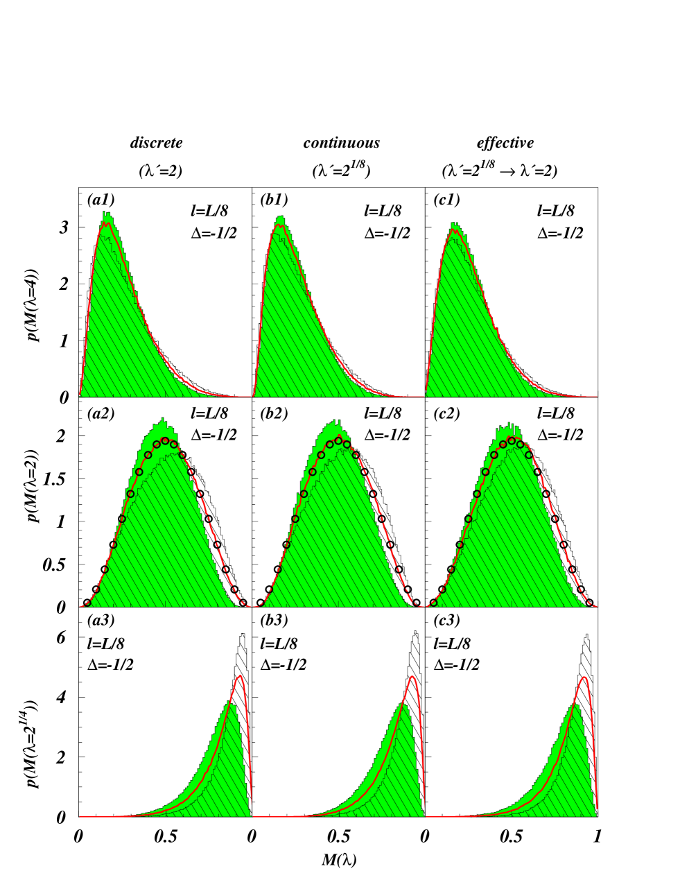
FIG. 1.: Scale-independent left-sided ($\Delta=-0.5$) multiplier distributions from a discrete (a1-3), a continuous (b1-3), and an effective, continuous-turned-discrete (c1-3) implementation of multiplicative cascade models; see text for model details. Solid curve: unconditional distribution $p(M(l;\lambda,-0.5)$; fully underlaid curve: conditional distribution $p(M(l;\lambda,-0.5)|0\leq M(\lambda l;\lambda,-0.5)\leq\lambda^{-1})$; hatched curve: conditional distribution $p(M(l;\lambda,-0.5)|\lambda^{-1}\leq M(\lambda l;\lambda,-0.5)\leq 1)$. The circled curve in (a2-c2) represents the parametrisation (11) with $\beta_{1}=\beta_{2}=3.2$.

FIG. 2.: $\lambda$-dependence of the Beta-distribution-(11) parameter $\beta_{1}$ for the unconditional left-sided (open stars) and centred (full stars) multiplier distributions resulting from the binomial weight distribution (10) with parameters $\alpha_{1}=0.3$, $\alpha_{2}=0.65$. The marked points have been calculated from least-square fits and the interpolating lines are to guide the eye.

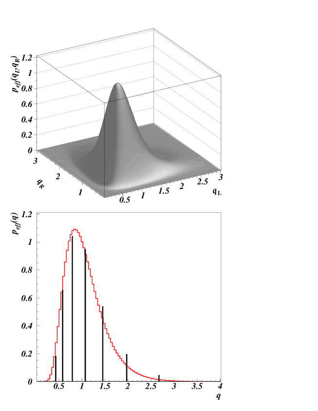
FIG. 3.: Effective bivariate (a) and projected (b) splitting function resulting from a continuous multiplicative cascade process translated into a binary discrete one. For comparison the weight distribution resulting from a naive $d$-fold convolution of the infinitesimal cascade generator is shown in (b) as appropriately rescaled bars.

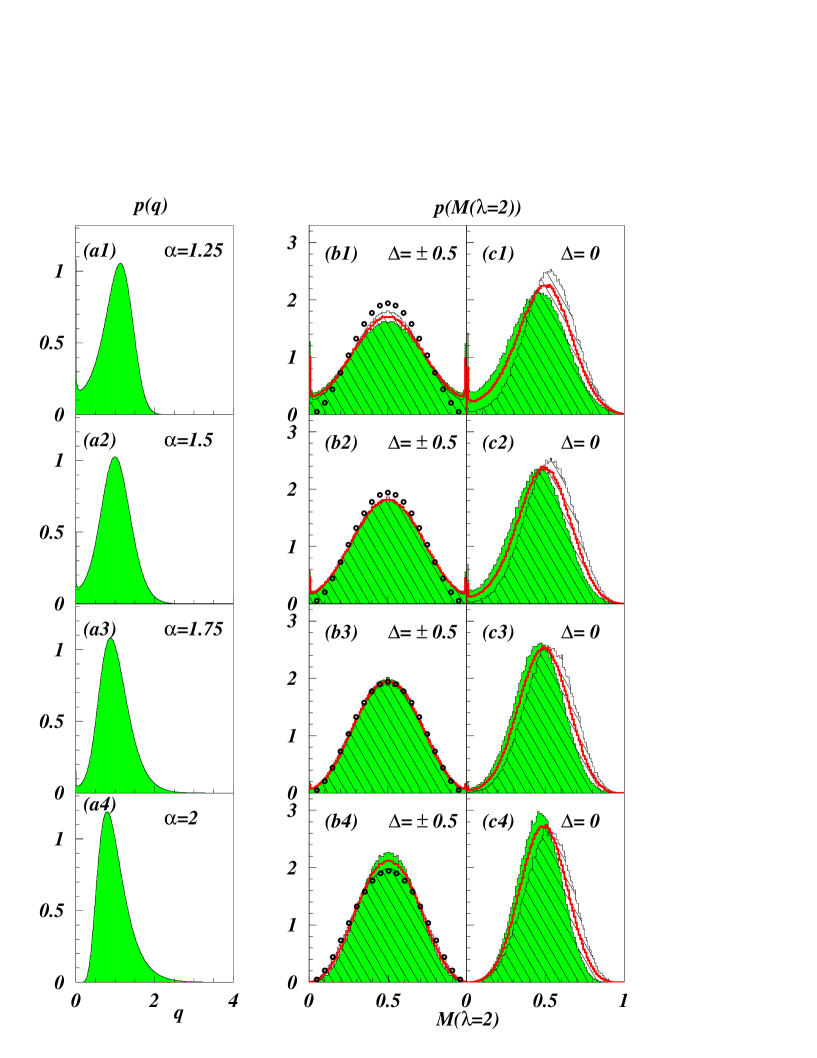
FIG. 4.: Various log-stable weight distributions (a) referring to a binary discrete multiplicative cascade process and their resulting left/right-sided (b) and centred (c) multiplier distributions.

- [1] K.R. Sreenivasan and R.A. Antonia, Ann. Rev. Fluid Mech. 29, 435 (1997).
- [2] M. Nelkin, Adv. in Physics 43, 143 (1994).
- [3] U. Frisch, Turbulence (Cambridge University Press, Cambridge, 1995).
- [4] V. Yakhot, Phys. Rev. E57, 1737 (1998).
- [5] V.I. Belinicher, V.S. L’vov, A. Pomyalov and I. Procaccia, J. Stat. Phys. 93, 797 (1998).
- [6] C. Meneveau and K.R. Sreenivasan, J. Fluid Mech. 224, 429 (1991).
- [7] G. Stolovitzky and K.R. Sreenivasan, Rev. Mod. Phys. 66, 229 (1994).
- [8] E.A. Novikov, Appl. Math. Mech. 35, 231 (1971); Phys. Fluids A2, 814 (1990).
- [9] A.B. Chhabra and K.R. Sreenivasan, Phys. Rev. Lett. 68, 2762 (1992)
- [10] K.R. Sreenivasan and G. Stolovitzky, J. Stat. Phys. 78, 311 (1995).
- [11] G. Pedrizzetti, E.A. Novikov and A.A. Praskovsky, Phys. Rev. E53, 475 (1996).
- [12] J. Molenaar, J. Herweijer and W. van de Water, Phys. Rev. E52, 496 (1995).
- [13] M. Nelkin and G. Stolovitzky, Phys. Rev. E54, 5100 (1996).
- [14] B. Jouault, P. Lipa and M. Greiner, Phys. Rev. E59, 2451 (1999).
- [15] B. Jouault, M. Greiner and P. Lipa, preprint chao-dyn/9812001, Physica D, in press.
- [16] Z. She and E. Leveque, Phys. Rev. Lett. 72, 336 (1994).
- [17] D. Schertzer and S. Lovejoy, J. Geophys. Res. 92, 9693 (1987).
- [18] D. Schertzer and S. Lovejoy, Physica A185, 187 (1992).
- [19] S. Kida, J. Phys. Soc. Japan 60, 5 (1991).
- [20] F. Schmitt, D. Lavallee, D. Schertzer and S. Lovejoy, Phys. Rev. Lett. 68, 305 (1992).
- [21] M. Greiner, J. Giesemann, P. Lipa and P. Carruthers, Z. Phys. C 69, 305 (1996).
- [22] E.A. Novikov, Phys. Rev. E50, R3303 (1994).
- [23] Z. She and E. Waymire, Phys. Rev. Lett. 74, 262 (1995).
- [24] F. Anselmet, Y. Gagne, E.J. Hopfinger and R.A. Antonia, J. Fluid Mech. 140, 63 (1984).
- [25] G. Samorodnitsky and M.S. Taqqu, Stable Non-Gaussian Random Processes (Chapman & Hall, New York, 1994).
- [26] M. Greiner, H.C. Eggers and P. Lipa, Phys. Rev. Lett. 80, 5333 (1998); M. Greiner, J. Schmiegel, F. Eickemeyer, P. Lipa and H.C. Eggers, Phys. Rev. E58, 554 (1998).