Lyapunov Exponent, Generalized Entropies and Fractal Dimensions Of Hot Drops

Abstract

We calculate the maximal Lyapunov exponent, the generalized entropies, the asymptotic distance between nearby trajectories and the fractal dimensions for a finite two dimensional system at different initial excitation energies. We show that these quantities have a maximum at about the same excitation energy. The presence of this maximum indicates the transition from a chaotic regime to a more regular one. In the chaotic regime the system is composed mainly of a liquid drop while the regular one corresponds to almost freely flowing particles and small clusters. At the transitional excitation energy the fractal dimensions are similar to those estimated from the Fisher model for a liquid gas phase transition at the critical point.

PACS numbers: 5.45+b, 5.70Jk

Infinite systems composed of particles interacting with an attractive plus, a shorter range, repulsive force have an Equation Of State (EOS) resembling a Van der Waals one [1], which exhibits phase transitions from solid to liquid and/or to gas. The features of the EOS of such a system are quite independent on the specific form of the two body potential, i.e. a sum of Yukawa’s or Lennard-Jones potential etc. A problem arises when the system is constituted of a finite number of particles $N$ and it is not confined in a box. In such a limit, it is not strictly correct to define a critical point, on the other hand it becomes very interesting to analyze how the system behaves as a function of its excitation energy. Intuitively we expect that at low excitation energies a transition, from solid-like state to liquid-like state, for a finite system should be very similar to the infinite case limit. This is so because at these low energies the attractive part of the potential is dominant and the system remains confined in a given, self sub-stained, volume. Thus it has sufficient time to develop correlations that are characteristic of such a phase transition[2]. In fact in this regime the Caloric Curve (i.e. the temperature $T$ of the system as a function of the excitation energy $E^{*}$) displays the standard ”rise-plateau-rise” pattern around the solid-like to liquid-like transition (i.e. the solid branch, the coexistence region and the liquid branch)[3]. At higher excitation energies the system is unable to remain confined and undergoes a fragmentation process. This kind of process is characterized by the appearance of a new degree of freedom, the one associated with the collective expansion. In this case, it has been found that many features of a thermodynamical liquid-gas transition are reproduced even if the system has mass as low as $A=100$ [4]. These features are mainly deduced from the analysis of asymptotic mass distributions and in particular one finds a power law in the mass yield for a given initial excitation energy. There have been also estimates of the critical exponents from data in nucleus-nucleus and cluster-cluster collisions [5, 6]. On the other hand the corresponding Caloric Curve does not show the usual increase in the temperature of the so called ”vapor branch” with the increase of the excitation energy, but instead a plateau is reached as soon as the systems enters the fragmentation regime[7]. The Maximal Lyapunov Exponent (MLE) has been studied in Classical Molecular Dynamics (CMD) for a 3 dimensional system composed of 100 particles and for different initial excitation energies. In [8] a maximum in the MLE was found for an initial excitation energy where a power law in the mass yield, intermittency signal, largest variance in the size of the biggest fragment[9, 4, 10] are also obtained. It is the purpose of this letter to strengthen and better characterize this result by analyzing the behavior of other important indicators of chaoticity, i.e. the asymptotic distance between trajectories [11, 12], the Generalized Renyi’s Entropies (GRE) and the fractal dimension [13]. We will solve the classical equation of motion (CEOM) for a system composed by 100 particles interacting through a 6-12 Lennard Jones potential in d=2 dimensions. Details on the method of solution of the CEOM and the preparation of the initial state are given in [14].

In order to calculate the MLE, we generate at time t=0, for each trajectory, a second one where we change the momenta of the particles by a small amount $d_{0}$ in momentum space. Following [8] we define a distance between trajectories $d(t)$  as:

$$d(t)=~{}\left(\frac{1}{N}\sum_{i=1}^{N}[a({\bf r}_{1}(t)-{\bf r}_{2}(t))^{2}+b({\bf p}_{1}(t))-{\bf p}_{2}(t))^{2}]_{i}\right)^{1/2}~{}~{}~{}\ ,$$ (1)

where ${\bf r},{\bf p}$ refer to the positions and momenta of $N$  particles at time $t$. Indices ${}^{\prime}1^{\prime}$ and ${}^{\prime}2^{\prime}$ refer to the two trajectories differing by $d_{0}$  at $t=0$ . $a,b$ are two arbitrary parameters which express the fact that the LE are independent of the particular metrics in the phase space[15]. For the purpose of this paper we will fix $a=0,b=1/m$ where m is the mass of the particles, i.e. distances in velocity v-space only. If we calculate numerically the time evolution of d(t) solving the CEOM, we observe an exponential increase followed by saturation in v-space [8, 11, 12]. The exponential increase of d(t) is associated to the MLE ${\hat{\lambda}}$ and it implies the following relation $\frac{d[d(t)]}{dt}=\hat{\lambda}d(t)$. But this rapid increase cannot last forever because the available v-phase space is limited, giving rise to a saturation of the inter trajectory distance in v-space. In order to describe this saturation, we can consider the previous relation as a first order term in an expansion in d(t), going to second order we get[11]:

$$\frac{d[d(t)]}{dt}=\hat{\lambda}d(t)-\alpha d^{2}(t)+..~{}~{}~{}~{}\ ,$$ (2)

where $\alpha$  is a constant greater than zero for fully developed chaos. Eq. (2) can be easily solved, giving:

$$d(t) = \frac{d_{\infty}d_{0}}{d_{0}+d_{\infty}e^{-\hat{\lambda}t}}$$ (3)

$$\hat{\lambda} = \alpha d_{\infty}~{}~{}~{}~{}~{}\ ,$$ (5)

where $d_{0}=d(t=0)$ and $d_{\infty}=d(t=\infty)$. Thus, eqs.(3,4) tell us that to characterize the entire time evolution of d(t), we need three quantities, $\lambda$, the asymptotic distance between trajectories $d_{\infty}$ and $\alpha$, but only two quantities are independent because of eq.(4). In particular since $\alpha$ is a constant we find that the LE are proportional to $d_{\infty}$. In ref. [11] this relation was supported from numerical simulation in Hamiltonian systems, similarly in ref.[12] for maps.

The MLE is proportional to the distance in v-space which provides a measure of the fluctuations. For instance for an infinite system in equilibrium as $t\rightarrow\infty$, the momenta of particles in event ’1’ are uncorrelated to those of event ’2’, and it is very easy to show that in such cases the $d_{\infty}$ is proportional to the variance in v-space. This is a very useful result which allows us to estimate the LE using the final distributions obtained either from the data or from the theory such as the thermodynamics. For example, for a classical Boltzmann gas the variance of the velocity distribution $\sigma$ is given by[1] :

$$d_{\infty}\propto\sigma=\left({\frac{3T}{m}}\right)^{1/2}~{}~{}~{}~{}~{}\ ,$$ (6)

where $T$ is the temperature of the gas measured in units of energy. For the infinite system the MLE is then an increasing function of the temperature of the system [11, 16]. On the other hand, in the case of a free expansion of a finite system (collective motion), $d_{\infty}=d_{0}$ holds, i.e. $\hat{\lambda}=0$.

In figure (1) we plot the MLE and the $d_{\infty}$ versus $E^{*}$ as obtained in our CMD simulations. The qualitative features are the same as those obtained in ref. [8, 11]. Both quantities plotted display a maximum even though at slightly different $\epsilon$. The decrease of the $d_{\infty}$ for large $\epsilon$, suggests that the particles having an initial kinetic energy larger than the binding energy escape quickly from the system without interacting. In fact if we compare this figure with the caloric curve displayed in ref.[7] we will notice that $d_{\infty}$ attains its maximum when the caloric curve reaches the plateau, which signals the state at which the dynamics of the system begins to be dominated by the collective radial flow. Similar considerations apply to the MLE. This supports also the idea of a limiting temperature that a finite system can sustain [17].

The maximum in the MLE signals a transition from a chaotic to a more ordered motion i.e. a motion in which the expansion collective mode is more an more important. For a finite system the main effect of collective motion is to suppress inter-particle collisions, in fact the higher the initial energy the faster the systems breaks and the smaller the final fragments are. Such a behavior resembles the one that has already been observed in [18] in a liquid to solid transition for the correlated cell model when changing the density. Notice indeed the similarity of the two cases. Small $\epsilon$ in our case corresponds to small $\rho$ in [18] i.e. the chaotic motion occurs in the liquid. At high $\epsilon$, we obtain a more ordered motion because of the collective expansion, while in [18] at high $\rho$ the system becomes a solid displaying regular trajectories which remains trapped within the volume determined by the neighboring particles.

If our simulations are followed for a long time, stable fragments will finally be formed. From the mass distributions we can estimate the GRE as follows. Define the probability of finding a fragment of mass i as the number of fragments $M(i,\delta)$, where $\delta$ is the mass resolution, divided the total number of fragments produced for a given event at that $\epsilon$. Thus

$$p(i,\delta)={\frac{M(i,\delta)}{\sum M(i,\delta)}}~{}~{}~{}~{}~{}\ .$$ (7)

The GRE are [13]:

$$S_{q}(\delta)={\frac{1}{1-q}}log({\sum_{i}<p_{i}>}^{q})~{}~{}~{}~{}~{}\ .$$ (8)

Where $<>$ denote the average over an ensemble and we take $q$ as an integer number. It is important to stress that the minimum mass resolution possible for finite systems is clearly $\delta=1$.

In figure (2a) we plot $S_{q}(\delta=1)$ vs. $\epsilon$ for $q=0-6$: a clear peak is observed. This peak is precisely in the region in which the MLE also shows a peak. Note that in the calculation we restricted the sum to those particles having mass larger than 2. If we keep smaller masses the peak remains even though it broadens.

From the knowledge of the GRE we can define the generalized dimensions (GD) as:

$$D_{q}={\frac{lim}{\delta\rightarrow 0}}{\frac{S_{q}(\delta)}{log\delta}}~{}~{}~{}~{}~{}\ ,$$ (9)

i.e. we study the way in which $S_{q}(\delta)$ scales with $\delta$[19]. In figure (2b) we show the fractal dimension ${D_{q}}$ vs. $\epsilon$. It is once again immediate to see a peak in ${D_{q}}$ ($q\geq 1$) in the same region in which MLE and ${S_{q}}$ displayed a peak. Finally in figure (3) we plot the ${D_{q}}$ vs. $q$ for various excitation energies. For illustration we discuss some limiting cases. For instance if the mass distribution is uniform, we easily get $D_{q}=1$ for all q. This is a trivial case which tells us that the entire space is uniformly covered and the $D_{q}$ are equal to the topological dimension 1. Another limiting case is when all the particles are concentrated in one bin (say mass 1) and zero otherwise. This gives $D_{q}=0$ which is the dimension of the space occupied i.e. the dimension of a point. It is also interesting to note that if the $p_{i}$s are different from $0$ for M contiguous bins only, then $D_{0}=1$ ,i.e. the Hausdorff dimension of a segment. A more interesting case is when the mass distribution is given by a power law. We can write such a mass distribution as $y(x)\propto x^{-\tau}$ where $x\epsilon[\epsilon,1]$, $x=i/N$ and $\epsilon$ is a small quantity related to the smallest possible mass that we can have. Following [13], taking the limits $\delta\rightarrow\epsilon\rightarrow 0$ gives, for $\tau<1$:

$D_{q}$=1 if $q<1/\tau$; $D_{q}$=$q(1-\tau)/(q-1)$ if $q\geq 1/\tau$

For instance, $\tau=0.5$ gives the GD as for the logistic map at r=4 [13], with $D_{q}$ continuous but its first derivative has a discontinuity at $q=2$ and this behavior is referred to as a first order phase transition. As we noticed before in our case we get a power law distribution for the excitation energy where the MLE and the GRE have a maximum. Since the power that we get is larger than 2 it is interesting to see what the behavior of the $D_{q}$ is in such a case which corresponds to a second order phase transition (at least in the infinite case limit). First we have simulated numerically a power law yield and the result is plotted in fig.(3) (full squares), with $A=100$ and $\tau=2.1$. The CMD results for $\epsilon=-0.75$(circles), where a power law in the mass distribution is obtained, are in good agreement with the simulation. We notice that the $D_{q}$ show no discontinuities at variance with the cases where $\tau\leq 1$. In order to test if this is a finite size effect we have simulated fragmentation in a simple percolation model whose properties are well studied. We find a similar behavior to the one discussed above at the critical percolation point and for very large sizes, more details will be discussed elsewhere. The $D_{q}$ are also plotted for the cases when $d_{\infty}$ has a maximum (open circles) and at high $\epsilon$ (open squares). The functional dependence of the $D_{q}$ with q suggests a multi fractal character of the probability distributions.

From these analysis the behavior of excited finite systems is greatly clarified. If we start with a cold (solid) drop of matter and begin to heat it up the Lyapunov exponent increases as well as the $d_{\infty}$. The first one is proportional to the rate at which the system explores phase space and the second to the available phase space. This trend changes as the rate of evaporation increases i.e when radial flow, the extra degree of freedom characteristic of the evolution of highly excited finite systems, starts to play a major role in the evolution. A maximum of both quantities is reached when the system approaches the critical region, i.e. when fluctuations are maximal and the final spectra contain both liquid-like and vapor like components. For even higher excitation energies both values decrease as a result of the fast fragmentation process and the transfer of chaotic (thermal) energy into ordered (radial flux) energy. A peak is also observed in the generalized Renyi entropies and in the generalized Fractal Dimensions ${D_{q}}$. The $D_{q}$ at the ’critical’ point for which a power law with $\tau\geq 2$ is obtained is a smooth decreasing function of $q$, at variance with the cases where $\tau\leq 1$.

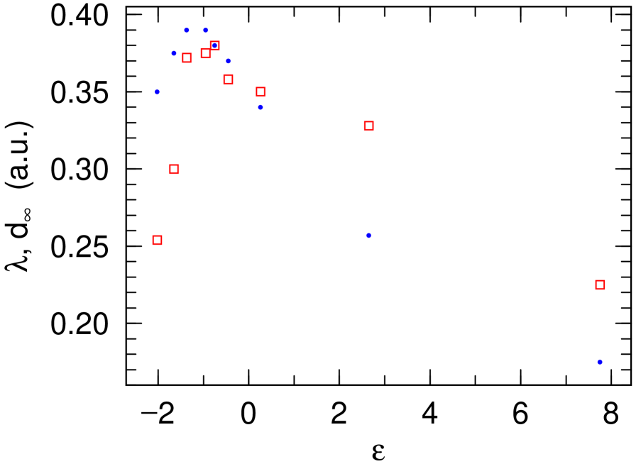
FIG. 1.: MLE (squares) and $d_{\infty}/4$ (dots) as a function of energy (in natural units $\epsilon$ [14]) for two dimensional L.J. drops with N=100 particles.

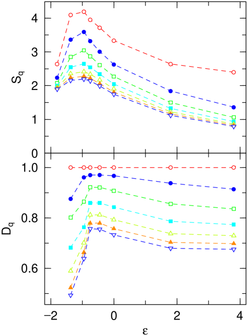
FIG. 2.: Generalized entropies (top) and fractal dimensions (bottom) vs. energy calculated from the asymptotic mass spectra for the same system as Fig.1. Open circles q=0 , full circles q=1, open squares q=2 , full squares q=3 , open triangles q=4, full triangles q=5, down pointing triangles q=6

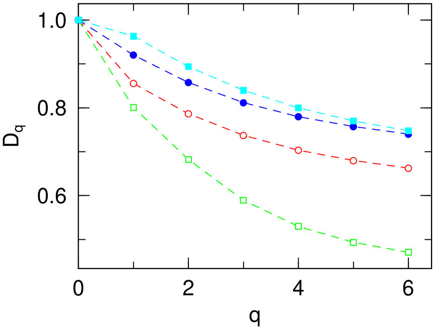
FIG. 3.: Generalized fractal dimensions at $\epsilon=-1.37$ (open circles), $-0.75$ (full circles), and $2.25$ (open squares). The full squares are obtained assuming a power law mass distribution.

REFERENCES

-
[1]
L. Landau and E. Lifshits, Statistical Physics, Pergamon,
New York,1980;
K.Huang, Statistical Mechanics, J.Wiley , New York, 1987, 2nd ed. - [2] S.K.Nayak, R. Ramaswamy, C. Chakravarty, Phys. Rev. E51, 3376 (1995).
- [3] P.Labastie and W. Wheten Phys.Rev.Lett.65,1567 (1990)
- [4] A.Bonasera, Phys.World 12,20 (1999); V.Latora, M.Belkacem and A.Bonasera, Phys. Rev. Lett. 73, 1765 (1994); P.Finocchiaro, M.Belkacem, T.Kubo, V.Latora and A.Bonasera, Nucl. Phys. A600, 236 (1996).
- [5] M.L.Gilkes et al. Phys.Rev.Lett. 73,1590(1994); P.F.Mastinu et al. Phys.Rev.Lett. 76,2646(1996); M.D’Agostino et al. Nucl.Phys.A650,329 (1999).
- [6] B.Farizon et al., Phys.Rev.Lett. 81,4108 (1998).
- [7] A. Strachan and C. O. Dorso Phys.Rev. C52, R632 (1998). A.Strachan and C.O.Dorso Phys.Rev. C59, 285 (1999).
- [8] A. Bonasera, V. Latora and A. Rapisarda, Phys. Rev. Lett. 75, 3434 (1995).
- [9] C.O.Dorso, V.Latora and A.Bonasera Phys.Rev.C60,34606 (1999).
- [10] X. Campi, J.of Phys. A19, 917 (1986); Phys. Lett. B208, 351 (1988)
- [11] A.Bonasera, V.Latora and M.Ploszaijck, Ganil preprint june 1996 (unpublished).
- [12] V.Baran, A.Bonasera chao-dyn/9804023.
-
[13]
B. Mandelbrot, The Fractal Geometry of Nature, Freeman,
San Francisco, 19:83;
J.L. McCauley, Chaos Dynamics and Fractals, Cambridge Nonlinear Science Series 2, Cambridge University Press 1993;
E. Ott, Chaos In Dynamical Systems, Cambridge University Press, England, 1993;
R.C. Hilborn, Chaos and Nonlinear Dynamics, Oxford University Press, New York, 1994.
M.Schroeder, Fractals, Chaos, Power Laws, W.Freeman and C.,USA,1991.
H.G. Schuster, Deterministic Chaos, VCH eds., Germany, 1995. - [14] C.O.Dorso and A.Strachan Phys. Rev. B54, 236 (1996); A.Strachan and C.O.Dorso Phys.Rev.C35, 775 (1997).
- [15] We remark that if the collective effects are important, then the calculations of the MLE become sensitive to the time when the second trajectory is generated. Here, we are always referring to the MLE as obtained by generating a second trajectory at [8].
- [16] I.Borzsak, A.Baranyai and H.Posch, Physica A229, 93 (1996).
- [17] R. Wada et al., Phys.Rev. C39,497 (1988).
- [18] C.Dellago, H.A.Posch, Physica A230, 364 (1996); C.Dellago, H.A.Posch and W.G.Hoover, Phys. Rev. E53, 1485 (1996).
- [19] Notice that even though the minimum possible mass is , when plotting vs. in log-log scale we can extrapolate to . We would like to stress that the range where the fit is performed , see eq(8), is limited due to the finiteness of the system.