On the dynamics of a self-gravitating medium with random and non-random initial conditions

Abstract

The dynamics of a one-dimensional self-gravitating medium, with initial density almost uniform is studied. Numerical experiments are performed with ordered and with Gaussian random initial conditions. The phase space portraits are shown to be qualitatively similar to shock waves, in particular with initial conditions of Brownian type. The PDF of the mass distribution is investigated.

1	Dept. of Mathematics, Stockholm University,
	SE-106 91 Stockholm, Sweden
2	Dept. of Numerical Analysis and Computer Science, Stockholm University/KTH,
	SE-100 44 Stockholm, Sweden
3	Niels Bohr Institute, Blegdamsvej 17,
	DK-2000 Copenhagen, Denmark

Submitted to Physica D

1 Introduction

In this paper we study the dynamics of a self-gravitating medium, the initial density of which is almost homogeneous, and of which the initial velocities of all fluid particles are small.

The study is performed in one spatial dimension where gravitational force is a Lagrangian invariant. The equations of motion for the density and velocity perturbations can therefore be written such that the net acceleration of fluid particles are Lagrangian quasi-invariant, if the perturbations are represented as discrete mass points moving on a stationary and uniform background. This system of particles is then brought forward in discrete time steps from one collision to the next, which, as shown already by Eldridge and Feix [7], permits the construction of an exact (up to round-off errors) and fast numerical integration scheme.

One reason to study the one-dimensional case is, that we wish to study the dynamics starting from initial conditions that are Gaussian random fields with power-law spectrum, and the statistical properties of these solutions. By analogy with recent work on the adhesion model [30, 33, 11], we then expect that there is a wide range of spatial scales in the solutions at late times. To get good statistics, while still resolving fully all details of the motion, a one-dimensional model is more convenient than simulations in two or three dimensions.

Our motivation to study gravitational dynamics with such random initial conditions is that this is as a model of structure-formation in the early universe, see [34, 25, 36]. We will return to a discussion of background material in cosmology in section 2. A second reason for a detailed study of one-dimensional case is then that, in general position, gravitational collapse accentuates asymmetries in the velocity and density fields. The first structures to form are blinis or pancakes, thin in one direction and of large extent in the two others. What we study can then be pictured as the one-dimensional dynamics of very large blinis, oriented parallel to one another and colliding and merging when moving under their mutual gravitational attraction. For very long times the tree-dimensional nature of the motion is no doubt important, but for some time after the first blinis form, the one-dimensional approximation should be appropriate. This point has recently been extensively discussed in [33], in the context of the adhesion approximation. The one-dimensional model can hence perhaps also give a quantitatively correct description of the clustering of mass as function of time as long as we consider the largest structures at every moment of time.

The main new results of this paper are as follows: we rederive the Rouet et al. mathematical model in a way which appear transparent to us, with particular emphasis on initially localized perturbations. We discuss the differences between structures observed on a uniform and homogeneous background, and those in a finite medium without a background. As has been observed previously [27, 28], phase space portraits, starting from ordered initial conditions, or random initial conditions, consist of smooth one-stream intervals (with ordered initial conditions), and short intervals with multi-stream solutions and high mass concentration. In particular, with Gaussian initial conditions of strong spectral support at low wave numbers, e.g. of Brownian type, we find qualitative similarities to the mass distributions in the adhesion model, i.e. ramps and mass concentrations of all sizes at all scales. We try to quantify the mass distribution by computing scaling exponents and mass histograms in octaves.

Recent mathematical investigations of finite self-gravitational systems, without a background, are [26] (ordered initial conditions) and [4] (random initial conditions, but of another class than we use), for a discussion of applications of this system to structure formation in the universe, see [12]. For Vlasov-Poisson equation in one dimension (mutual repulsive interaction), see [20].

The paper is organized as follows. In section 2 we summarize standard material in cosmology, and discuss references to recent observational data on the anisotropies of the cosmic microwave background radiation. In section 3 we derive the Rouet et al. solution of 1D self-gravitating systems, and discuss initial conditions appropriate for our system and admissible boundary conditions. In section 4 we study the dynamics starting from ordered and random initial conditions, and in section 5 we investigate properties of the mass distribution. In section 6 we sum up and discuss our results.

2 The cosmological and observational setting

In our immediate neighborhood today, the universe is neither homogeneous nor isotropic. Sources of electro-magnetic radiation in any frequency band are distributed in a markedly random and clustered manner over the sky. On the other hand, at large scales the universe is generally taken to be homogeneous and isotropic. The hypothesis of an early almost homogeneous and isotropic state of the universe rests on that it agrees with the whole body of theory of the hot Big Bang, and with the observed 3K black-body background radiation. It is therefore natural and standard to assume that the structures observed today are due to instabilities in an initially almost homogeneous self-gravitating medium [34, 25, 36].

The study of such instabilities has a long pre-history, going back already to Newton [21]. The first quantitative investigation of the instability in a static medium with non-zero pressure was performed by Jeans [14], who derived his famous formula that perturbations of wave-length larger than $\lambda_{J}=v_{s}\sqrt{\pi/G\rho}$ are unstable, where $v_{s}$ is the sound speed, $G$ the gravitational constant and $\rho$ the density. Such perturbations hence grow exponentially in time (in the Jeans theory), while perturbations of smaller wave-length oscillate and do not grow. The Jeans length can be related to a Jeans mass of $M_{J}=\frac{4\pi}{3}\rho\lambda_{J}^{3}$. In an almost homogeneous gas, regions of increased density with mass larger than the Jeans mass collapse gravitationally, while concentrations of smaller mass oscillate acoustically.

While Jeans’ analysis immediately applies to gravitational collapse of a finite object, it is not complete when referring to a medium of infinite extent. Since a sufficiently large mass will always be unstable, the unperturbed state assumed in the Jeans formula, an infinite self-gravitating medium with gravitational self-interaction and constant density, cannot exist in classical physics. On the other hand, in general relativity the Friedmann solutions to the Einstein equations describe unbounded universes with spatially constant density. These solutions are given in terms of a cosmological length scale $a$, which changes with cosmological time $t$. On sufficiently small length scales (much less than $a$), and on sufficiently short time-scales (faster than $\frac{a}{\dot{a}}$) general relativity is well approximated by Newtonian gravity, and Jeans’ analysis of an infinite medium is hence well-founded in this way.

The linear theory of small perturbations around the Friedmann solutions in general relativity was developed by Lifshitz, and is described in detail in Weinberg [34] and Zeldovich & Novikov [36]. If we assume a hydrodynamic description of the matter fields, the perturbations can be classified as scalar, vector and tensor. The last ones correspond to gravitational waves, which have no counterpart in the classical theory, and will be left aside in the following.

Although the relevant calculations are involved, to a considerable degree the results can simply be described by introducing the co-moving wavelength

$$q(t)=q(t_{0})\frac{a(t)}{a(t_{0})}$$ (1)

Then the perturbations in density and proper velocity (scalar and vector perturbations) grow as

$$f_{k}(q(t),t)\approx e^{\int_{t_{0}}^{t}\lambda_{k}(q(t^{\prime}),t^{\prime})dt^{\prime}}f_{k}(q(t_{0}),t_{0})$$ (2)

where $\lambda_{k}(q,t)$ is the instantaneous growth rate in the Jeans theory of wave-vector $q$ at time $t$, and $k$ labels the linear modes. Equation (2) does not agree completely with Lifshitz’ full solution, but is quite close in standard cosmological models. For an extended discussion, see [36].

The linear modes can be classified into decaying modes, which are fields of incompressible proper velocities, and growing modes, which are linear combinations of density modes and potential proper velocities. If a mode actually grows or decays at time $t$ also depends on whether the co-moving wave-length is smaller or greater than the instantaneous Jeans length. On sufficiently large scales, the perturbations surviving the linear regime are coupled density and potential proper velocity fluctuations.

The outcome of these considerations is that at length scales much smaller then the radius of the Universe, but much larger than the Jeans’ length, structure formation, as long as the solutions are single-stream, is governed by the following system of equations:

$$\left\{\begin{array}[]{l}\displaystyle{\partial_{t}\rho+3\frac{\dot{a}}{a}\rho+\frac{1}{a}\overrightarrow{\nabla}\cdot({\rho}\overrightarrow{u})=0}\\ \\ \displaystyle{\partial_{t}\overrightarrow{u}+\frac{\dot{a}}{a}\overrightarrow{u}+\frac{1}{a}(\overrightarrow{u}\cdot\overrightarrow{\nabla})\overrightarrow{u}=-\frac{1}{a}\overrightarrow{\nabla}\psi}\\ \\ \displaystyle{\nabla^{2}\psi=4\pi Ga^{2}(\rho-\rho_{b})}\end{array}\right.$$ (3)

If we also assume that initial rotational proper velocity fluctuations have been damped out in the linear decay, then $\overrightarrow{u}$ is a potential field at some time $t_{0}$. $\psi$ is the gravitational potential generated by the source $\rho-\rho_{b}$. We note that $\rho-\rho_{b}$ can be both negative and positive, and is zero on average. On short time scales we can take $a$ constant, and by a change of scale we can set it equal to one. On the kinetic level the system is then described by the following Jeans-Vlasov-Poisson equation, valid also after caustic formation:

$$\left\{\begin{array}[]{c}\displaystyle{\partial_{t}f+\frac{\overrightarrow{p}}{m}\cdot\overrightarrow{\nabla}_{x}f-\overrightarrow{\nabla}\psi\cdot\overrightarrow{\nabla}_{p}f=0}\\ \\ \displaystyle{\rho=\int f\,d\,\overrightarrow{p}\quad\overrightarrow{u}=\frac{1}{\rho}\int\frac{\overrightarrow{p}}{m}f\,d\,\overrightarrow{p}\quad\nabla^{2}\psi=4\pi G(\rho-\rho_{b})}\end{array}\right.$$ (4)

The initial conditions of equations (3) and (4) can be taken to be the fluctuations at some stage of linear growth. It is a remarkable fact that the fluctuations at one particular time during linear growth are in fact observable in the fluctuations of the $3K$ blackbody background radiation [23, 24, 32, 15]. At red-shift $z\simeq 1000$ (age of the Universe $10^{5}$ years), photons fell out of thermal equilibrium with electrons and nuclei; what is observed today as $3K$ black body radiation is the red-shifted spectrum of photons that were in equilibrium with matter at that time. COBE observations measure the temperature of the blackbody radiation with a beam width of $7^{\rm o}$, and detect mean square variations of about $30\mu K$ (one part in $10^{5}$). Laid out in the sky, COBE can thus be said to distinguish a spherical grid of $50\times 50$ patches, i.e. a decade and a half in each direction. Experiments in the near future (MAP, Planck Surveyor) are expected to increase the angular resolution of COBE by more than one order of magnitude. Over the range of COBE, observations are in agreement with the Harrison-Zeldovich[13, 35] prediction of Gaussian initial density fluctuations with spectrum [32, 17]:

$$P(k)=Ak^{n}\qquad n\simeq 1$$ (5)

At scales smaller than about $1^{\rm o}$, theoretical arguments predict deviations from (5). In cold dark matter-dominated models these are determined by the CDM transfer function, which at intermediate scales, in the present universe in the range $10-50h^{-1}\hbox{Mpc}$, gives a plateau where fluctuations are also Gaussian as in (5), but with $n\simeq-1$ [3]. We remark that in practically all cosmological models, the spectrum (5) is not expected to be valid in an arbitrary wide range, but to be modified at smaller scales. For further recent discussions on the assumed limits of validity of (5) and prospects of experimental observations of such deviations, see e.g. [32, 15, 19].

3 The generalized Zeldovich solution: a Lagrangian integrable model

We now turn to a Lagrangian integration scheme where initial mass density $\rho$ is concentrated on a discrete set of particles. The algorithm which we are going to describe was invented in plasma physics (i.e., equation (4) with the opposite sign of $G$) in the early ’60ies, and already previously used in simulations of one-dimensional self-gravitating systems [5, 27, 28]. The derivation we will give stresses localized initial perturbations. Boundary conditions are hence those of an unperturbed quiescent state to the left and the right of the perturbation. As the perturbation develops it will typically spread, and move into the quiescent state, thus inducing that to move. The main ingredient in the derivation is a regularisation of the differences between the (formally divergent) forces pulling the particle to the left and to the right. Since the physical meaning of an infinite classical self-gravitating system is that of an approximation (on sufficient small scales) to a system governed by general relativity, and since the speed of propagation of the gravitational interaction in general relativity is finite, localized perturbations are relevant in this problem.

We now take space one-dimensional. The mass density distribution corresponding to a system of point-like particles is specified by:

$$\rho(x,t)=\sum_{k}m_{k}\delta(x-x_{k}(t))$$ (6)

We require that the average density of the point-mass system is the same as the background density, i.e.

$$\hbox{Lim}_{L\to\infty}\left[\frac{1}{2L}\sum_{k:x_{k}(t)\in[-L,L]}m_{k}\right]\,=\,\rho_{0}\,=\,\rho_{b}$$ (7)

and that the perturbation is localized in a weak sense, such that as $L$ tends to infinity the measure of the point masses in $[L,L+1]$ tends to the uniform measure in the same interval, with convergence faster than $\frac{1}{L^{2}}$. The one-dimensional gravitational potential is formally given by

$$\psi(x,t)=2G\int dy|x-y|(\rho(y,t)-\rho_{b})\qquad\hbox{({\it formally})}$$

With the initial conditions under consideration the integral is convergent at infinity. The regularisation referred to in the beginning of this section is therefore to take

$$\psi(x,t)=2G\,\hbox{Lim}_{L\to\infty}\left[\sum_{l:{x}_{l}\in[-L,L]}m_{l}|x-x_{l}|-\rho_{b}\frac{(x-L)^{2}+(x+L)^{2}}{2}\right]$$ (8)

where the limit exists by assumption. As now $\psi$ is a known and well-defined function of position, the equations of motion of the point masses are

$$\ddot{x}_{k}=-\frac{\partial\psi(x)}{\partial x}|_{x=x_{k}}=-2G\,\left[\hbox{Lim}_{L\to\infty}\sum_{l:{x}_{l}\in[-L,L]}m_{l}\hbox{sign}(x_{k}-x_{l})-2\rho_{b}x_{k}\right]$$ (9)

with initial conditions $x_{k}|_{t=0}=x_{k}(0)$ and $\dot{x}_{k}|_{t=0}=u_{0}(x_{k}(0))$. Equation (9) expresses that the force acting on particle $k$ is equal to the difference of net mass, in excess of the background, to the right and to the left of that particle. Hence, were $L$ infinite, it would formally be the sum of four terms (two with positive and two with negative signs), each of which would be infinite. Our regularisation acts on the net force to the left and to the right separately, by the requirement that the initial perturbation is localized.

With periodic boundary conditions our regularisation would not give a unique answer since the limit (8) would not exist. One could instead regularise separately the net force from particles and net force from the background, for instance by taking the net force of each kind initially to be zero, or assuming that the gravitational force actually is of finite range, and then take the limit when that range increases. Using (9) necessarily assumes implicitly a regularisation, of which ours is a physically transparent one, at the price that we consider only sufficiently localized perturbations.

We now want to transform (9) to the Eldridge-Feix scheme. The acceleration acting on point mass $k$ at the initial time is

$$a(x_{k}(0),0)=-2G\,\left[\hbox{Lim}_{L\to\infty}\sum_{l:x_{l}\in[-L,L]}m_{l}\hbox{sign}(x_{k}(0)-x_{l}(0))-2\rho_{b}x_{k}(0)\right]$$ (10)

From (9) follows that as long as no other particle overtakes particle $k$ we have the simple evolution law

$$\ddot{x}_{k}(t)=a(x_{k}(0),0)+4G\rho_{b}(x_{k}(t)-x_{k}(0))\qquad\hbox{(time $t$ before collision)}$$ (11)

When particle $l$ overtakes particle $k$, the gravitational force acting between them changes sign. We may therefore write the equations of motion at an arbitrary time $t$ as

$$\begin{array}[]{l}\displaystyle{\ddot{x}_{k}(t)=a(x_{k}(0),0)+4G\rho_{b}\left(x_{k}(t)-x_{k}(0)\right)+}\\ \\ \displaystyle{-2G\sum_{l}m_{l}\left[\hbox{sign}(x_{k}(t)-x_{l}(t))-\hbox{sign}(x_{k}(0)-x_{l}(0))\right]}\\ \\ \end{array}$$ (12)

If units are chosen such that $4G\rho_{b}=1$ (see below), the mapping from one collision to the next is then

$$\begin{array}[]{l}\displaystyle{x_{k}(t^{i+1}_{coll})=x_{k}(t^{i}_{coll})-a_{k}(t^{i}_{coll})+}\\ \\ \displaystyle{+\frac{a_{k}(t^{i}_{coll})+\dot{x}_{k}(t^{i}_{coll})}{2}\exp(t-t^{i}_{coll})+}\\ \\ \displaystyle{+\frac{a_{k}(t^{i}_{coll})-\dot{x}_{k}(t^{i}_{coll})}{2}\exp(t^{i}_{coll}-t)}\end{array}$$ (13)

where $\dot{x}_{k}(t^{i}_{coll})$ and $a_{k}(t^{i}_{coll})$ are the velocity and the acceleration felt by the $k$’th particle at the preceding collision.

4 Numerical experiments

A characteristic scale in time is set by the Jeans’ frequency, related to the gravitational constant $G$ and the mean density $\rho_{0}$ by

$$\omega_{J}=\sqrt{4G\rho_{0}}$$ (14)

In the following we will measure time in units of $\omega_{J}^{-1}$. Since the mean density is equal to the background density $\rho_{b}$, this means that we choose a scale in time such that the value of the product $4G\rho_{b}$ in (12) is one.

The model of self-gravitating particles without pressure is valid on spatial scales much greater than the Jeans length $\lambda_{J}$. The intrinsic spatial scale $\lambda_{J}$ is thus for us zero. Characteristic spatial scales can hence only come from the initial conditions. If the initial perturbation is ordered (smooth function of spatial coordinate), and in analogy with (7) and (9) has support on an interval $[-L,L]$ then all scales can be measured in terms of $L$. Temporal and spatial scales $\omega_{J}^{-1}$ and $L$ imply however a velocity scale $L\omega_{J}$, and we can therefore separate ordered initial velocity perturbations as to if they are large or small compared to $L\omega_{J}$. An initial density perturbation $\delta\rho$ is naturally measured in units of the mean density. We choose to normalize mass in terms of the mass $M$ initially involved in the perturbation, which means that $\rho_{0}$, and therefore $\rho_{b}$, is $\frac{M}{2L}$. The constant $G$ in (12) is $\omega_{J}^{2}\frac{L}{2M}$, in our units hence $\frac{1}{2}$.

The explicit formula (13) allows immediately for a fast numerical scheme with operations count ${\cal O}(N)$ per collision, where $N$ is the number of particles; this is scheme of Eldridge and Feix[7]. Elsewhere we will discuss an asymptotically more efficient version of the algorithm with an operation count of ${\cal O}(\ln N)$ per collision [1]. We note that the computer time needed to advance the system up to time $t$ is proportional to the product of the number of operations per collision and $N_{coll}(t)$, the number of collisions up to time $t$. If with initially smooth velocity and density perturbations, represented as $N$ discrete particles, the mean time between collisions depend on $N$ as $\frac{1}{N}$, then in the algorithm used here the operations count in advancing the system up to intrinsic time $t$ would be $N^{2}$. However, due to stretching and separation, the discretization becomes gradually a less accurate description of the smooth field to be approximated; this effect is far from uniform in phase space, and the putative ${\cal O}(N^{2})$ operation count therefore only holds approximately at an initial stage.

In fig 1 we show an initially smooth velocity perturbation (insert) of sinusoidal shape in the interval $[-1,1]$. The initial density perturbation is zero. The full system thus consists of a uniform stationary background with density $\rho_{b}$, and a number of particles as in (6), distributed uniformly with respect to the same density, and at rest outside the interval. As long as no particle from the inside has reached the boundaries all three terms on the right-hand side of equation (12) remain unchanged for a particle outside $[-1,1]$, and these particles thus remain at rest. The main figure in fig 1 show the solution at time $4.0\,\omega_{J}^{-1}$, at a resolution where obviously the continuum description is still applicable, and where no particle from inside has reached the boundaries. In phase space the distribution has support on a curve of spiral shape. If initial velocity is large or compared to $L\omega_{J}$, the fastest particles typically reach the boundaries before a spiral is formed, while if initial velocity is much smaller than $L\omega_{J}$ one or more turns of the spiral form before any particles reach the boundaries. These observations have already been made by Rouet et al [27, 28], and show a qualitative difference in the solutions depending on the initial kinetic energy.

In fig 2 we show the development of the system in fig 1 at successive later stages. The most distinct features are the formation of a high-density cluster in the middle, and two expanding high-density fronts to the left and right, but with very low density in between. The two fronts form when particles from the interval collide with particles that were initially at rest. The first particles to do so overtake the same mass in resting particles and background, and will therefore feel no change in the acceleration. The resting particles that have been overtaken will on the other hand feel an acceleration towards the front that has passed. They will hence start moving towards the front, making non-leading particles in the front overtake more background than particles, and therefore also feel an increased acceleration. Both these effects lead to a high density concentration at the front, large force gradients, and strong stretching in phase space. In fact, it is clear that with the resolution used in fig. 2, at the fronts the continuum description is already lost.

In the center of the middle cluster the density is several times the background, and the spirals are round, as in dynamics without the background, while in the outer parts, where $\delta\rho$ is comparable to $\rho_{b}$, the spirals are deformed, as above on fig 1.

We now turn to random conditions. We made three different choices of velocity as function of spatial position: Brownian motion; fractional Brownian motion with Hurst exponent equal to zero, and white noise. All three are random Gaussian fields with power law spectra as in eq. (5), of which we choose white noise and Brownian motion because they are Markov processes, and have been investigated in the context of the adhesion approximation [30, 31], white noise also as a reference case, because it has earlier been investigated by Rouet and collaborators [27, 28], and the fractional Brownian motion as an interesting intermediate case.

The translation between exponents in (5) (density perturbations in 3D) and our initial conditions (velocity perturbations in 1D) is as follows: a Gaussian random function $f$ with stationary increments has second order correlation function $<|f(x+l)-f(x)|^{2}>\sim l^{2h}$, where the Hurst exponent $h\in[0,1[$ is related to the scaling exponent $n$ of the spectrum $E(k)\sim k^{n}$, through $2h+n+(D-1)=-1$. A scaling exponent $n_{1D}$ in $1D$ is therefore, for these purposes, analogous to a scaling exponent $n_{3D}=n_{1D}-2$ in 3D. A density perturbation $\delta\rho_{k}$ is in the linear regime on the other hand tied to a velocity perturbation $v_{k}\sim k\rho_{k}$. We therefore have $n^{(v)}=n^{(\rho)}+2$, and combining the two relations $n^{(v)}_{1D}=n^{(\rho)}_{3D}$. Our intermediate case with Hurst exponent equal to zero hence corresponds to the Bardeen-Bond-Kaiser-Szalay intermediate spectrum with $n^{(\rho)}_{3D}=-1$, and will in the following be referred to as BBKS initial conditions. White noise and Brownian motion correspond to $n^{(\rho)}_{3D}=0$ and $n^{(\rho)}_{3D}=-2$.

                        

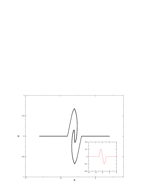
Figure 1: Velocity field vs. position at time $t=4.0\,\omega_{J}^{-1}$. Number of particles is $N=15\times 10^{3}$, initial sinusoidal conditions in lower right corner insert.

                        

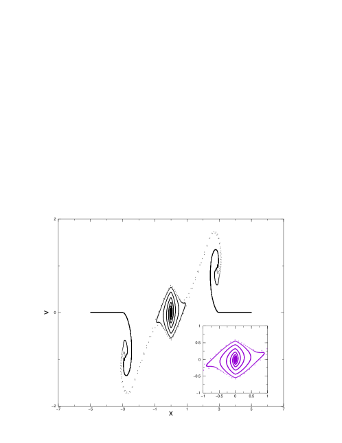
Figure 2: Velocity field vs. position of the system in fig. 1 at a later time, well into the non-linear regime ($t=11.08\,\omega_{J}^{-1}$). The insert is a blow-up of the central region. Three high-density peaks are clearly developed.

Gaussian random fields are conveniently generated in the Fourier space representation. At time $t=0$ particles are uniformly distributed on an interval of size $\ell$ with unit spacing $\Delta x=\ell/N$ and velocity

$$v(x)=\Sigma_{k}v_{k}e^{ikx}$$ (15)

The sum over $k$ extends from $-\pi\,/\,\Delta x$ to $\pi\,/\,\Delta x$ in steps of $2\,\pi\,/\,\ell$ and $v_{-k}=v_{k}^{*}$. The Fourier components of positive $k$ are then chosen as a random Gaussian independent variables with variances:

$$<|v_{k}|^{2}>=\frac{\,\,k^{-2h-1}}{2\,\Delta x}$$ (16)

The field generated by (15) and (16) will be periodic with period $\ell$. If $h$ is in the interval $[0,1[$ the field will have stationary increments on length scales much less than $\ell$, and on these scales approximate a Fractional Brownian motion with Hurst exponent $h$, while if $h$ is in the interval $]-1,0[$ the field itself will be stationary on length scales much less than $\ell$, and approximate the derivative of a Fractional Brownian motion. We choose $\ell=2L$, so that particles are initially distributed in a box $[-L,L]$.

We will now discuss units of time and space with random initial conditions. One scale is $2L$, another is the ultra-violet cut-off $l_{UV}$, which in our case is at least as large as the initial particle distance $\Delta x$, and a third is an infra-red cut-off $l_{IR}$, which is not larger than $2L$. With $h$ in the interval $[0,1[$ we have in law

$$v(x+l)-v(x)\sim v_{UV}(\frac{l}{l_{UV}})^{h}$$ (17)

where $v_{UV}$ is the size of typical velocity fluctuations on the ultra-violet cut-off scale. The typical overturning time at scale $l$ is then

$$t_{l}\sim\frac{l_{UV}}{v_{UV}}(\frac{l}{l_{UV}})^{1-h}\qquad h\in[0,1[$$ (18)

The time $\frac{l_{UV}}{v_{UV}}$ can be measured in units of inverse Jeans’ frequency, and be small or large in those units. Equation (18) then predicts that the characteristic time to form a structure of size $l$ increases with $l$, such that small scales form first. At sufficiently large scales $l$ the initial velocity fluctuations will be small compared to $l\omega_{J}$, and we hence expect to see the central spiral structure of figs 1 and 2, but not much of the fronts.

On the other hand, if the spectral exponent is larger than $-1$ (Hurst exponent less than zero), then the initial velocity field is homogeneous, characterized by a rms velocity $v_{RMS}$, which is on the order of $v_{UV}$, and we therefore expect the simpler result $t_{l}\sim\frac{l_{UV}}{v_{RMS}}(\frac{l}{l_{UV}})$. At scales much larger than $l_{UV}$ velocity fluctuations are again much smaller than $l\omega_{J}$, and we therefore expect mainly to see the central spiral structures of fig 1 and fig 2. We remark that if we reason by analogy, and assimilate these structures to shock waves in the adhesion model, which trap fast particles, then the characteristic times will be longer, and in fact again of the form (18). The turn-over time $t_{l}$ then grows faster then linearly with $l$ [11, 10]. Unfortunately our present resolution is not sufficient for a precise determination the typical size as function of time and of the temporal development of the spectral shape of the perturbations.

In figs. 3, 4, 5, 6 we show the phase space portraits with Brownian motion, white noise and BBKS initial conditions, respectively. As expected, we see many spiral structures, small and large, and fronts at the left and right boundaries, except in fig. 4, included as a consistency check (see below). In qualitative agreement with the adhesion model, we also see “ramps” with low density, and where velocity is an increasing function of position, interspersed with regions of high density. By visual inspection of an agglomeration of a certain scale, it appears that the velocity to the right of such an agglomeration is less than on the left, such that velocity has negative gradient through the agglomeration, just as in shocks in the adhesion model. This picture is however complicated by the fact that there are agglomerations of different sizes, and that they are not simply ordered from left to right. A certain stretch of phase space, say just to the left of some structure, is on some other scale included inside a much larger structure; this effect appears to be especially pronounced with Brownian motion initial conditions. In the adhesion model such microstructures are of course hidden inside the shocks.

The difference between figs. 4 and 5 is that in fig. 5 we include, following our general approach, a medium of quiescient particles to the right and left. As in fig. 2 we then find two expanding fronts, where the particles of initial velocities around $v_{RMS}$ in the interval collide with the particles initially at rest. To show that the fronts do not qualitatively change the dynamics in the central region, we show for comparison in fig. 4 a system with only background outside the interval. Particles that escape the central interval are then accelerated outwards by the anti-harmonic force in (12), and give phase space portraits where velocity $v$ is an increasing function of position $x$ outside the interval.

Another way to eliminate the fronts would be to take a perturbation which is similar to white noise, but of which the envelope would go smoothly to zero outside an interval of length $2L$, which can be achieved with essentially flat spectrum at wave numbers larger than $\frac{1}{2L}$. For Brownian and BBKS initial conditions we do not have to worry about the fronts. Without changing any many-point statistics we can constrain a realization using (15) and (16) to vanish at one point, say $x=-L$, and then by periodicity also at $x=L$. By (17) the typical velocities in the center of the interval $[-L,L]$ will then be much larger than at the boundaries, and the most prominent structures are found there.

                        

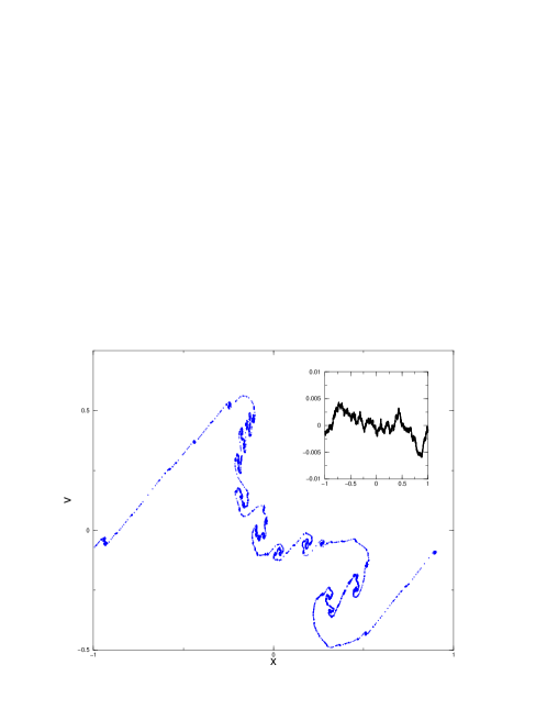
Figure 3: Velocity field vs. position at time $4.76\,\omega_{J}^{-1}$, starting from single-speed Brownian motion initial conditions (small upper right insert). Number of simulated particles is $N=8192$.

                        

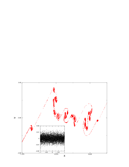
Figure 4: Velocity field vs. position at time $7.37\,\omega_{J}^{-1}$, starting from single-speed white noise initial conditions (lower insert). The model is modified, as described in the main text, to contain only background and no particles outside the interval of the initial perturbation. Number of simulated particles is $N=8192$.

                        

Figure 5: Velocity field vs. position at time $7.37\,\omega_{J}^{-1}$, starting from single-speed white noise initial conditions as in fig. 4 inside the interval of the perturbation, and quiescient particles to the right and left thereof. Note the formation of fronts as in fig. 2. Number of particles initially involved in the perturbation, with total mass one, is $N=8192$, and the total number of simulated particles, including the ones to the left and right, is $16384$.

                        

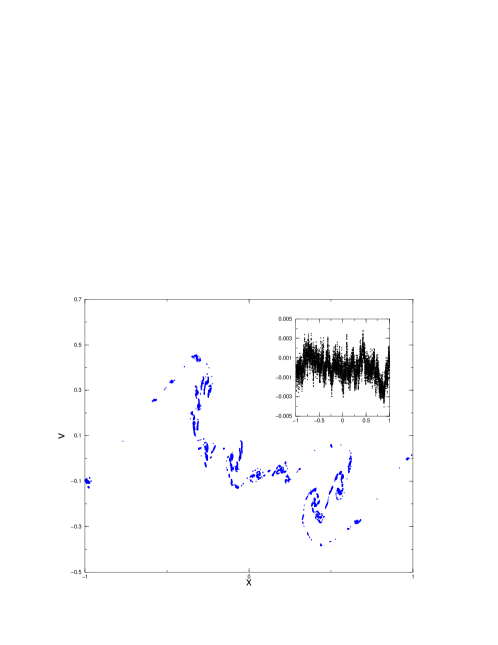
Figure 6: Velocity field vs. position at time $t=6.7\,\omega_{J}^{-1}$ starting from single-speed BBKS initial conditions (upper right insert). Number of simulated particles $N=8192$.

To quantify how accurate is a finite-particle description we looked at PDF of the inter-particle distances at different times. In fig. 7 we show the PDF of the inter-particle distances to the power one-half (insert on the right). In each case a peak is clearly observed: the positions of these peaks are independent of the initial realizations and evolution time. The main plot in fig. 7 shows the PDF of the rescaled quantity $\Gamma=(\frac{dx}{\beta^{h}})^{1/2}$ where the constant $\beta=0.6$ was obtained by a numerical fit. We have no good explanation of the observed scaling behaviour at this point.

                        

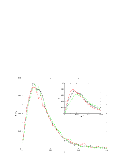
Figure 7: Insert on the right: the PDF of the inter-particle distances to the power $1/2$, for Brownian initial velocities (squares, $t=6.4\omega_{J}^{-1}$), BBKS (circles, $t=7.5\omega_{J}^{-1}$) and white noise (triangles up, $t=8.1\omega_{J}^{-1}$). Main figure: PDF of $\Gamma$, where $\Gamma=(\frac{dx}{\beta^{h}})^{1/2}$ and $\beta=0.6$.

5 Mass analysis

Qualitatively, the velocity field recalls the results obtained in the framework of the adhesion model [10, 30, 33], where “ramps” appear that separate shock regions where fully inelastic collisions among the Lagrangian particles occur. It is interesting to try to introduce quantitative characteristics of the mass distribution in order to make a closer comparison.

One main result of [30] and [2], is that for $h\in[0,1[$ the inverse Lagrangian map, initial versus final position, has a bifractal structure, similar to that of the Devil’s staircase construction using the standard triadic Cantor set. Except for a set of measure zero, all Lagrangian initial points land on shocks, which in Eulerian coordinates are at definite shock locations, and where therefore all of the mass is concentrated. The number density per unit length of shock locations holding mass $m$ is in a well-defined range distributed as a power-law $m^{-h-1}$. Most mass therefore lies in the largest shocks formed at a given time, but the number of smaller shocks is divergent. For the Brownian motion initial condition it can be proven, and for the other cases it is conjectured, that Eulerian shock locations are almost surely dense. Most of these shocks are still small. However, since all mass initially uniformly distributed after an arbitrarily short time falls into a shock, the mass contained in an interval after a finite time is in this model only made up of the mass in the shocks actually inside the interval. The mass measure of the adhesion model with these initial conditions is therefore bifractal, which can be quantified by the scaling exponents of its moments

$$M(q,l)=\Sigma_{i=1}^{B}\,p(x_{i})^{q}\,l\sim l^{\tau(q)}$$ (19)

where $l$ is the length of the coarse-graining mesh, $B$ is the number of boxes in the mesh, and $L=Bl$. The sum is normalized such that $\tau(1)=1$ and $\tau(0)=0$. At sufficiently large $q$, where the threshold lies at $h$, the sum in (19) is dominated by a small number of terms, corresponding to the intervals containing the larger shocks. The exponent $\tau$ in this range is then one. At small $q$ (19) would instead be dominated by almost empty intervals, each of which carries a mass $l^{\frac{1}{h}}$, and of which there would be $l^{-1}$ in number. The scaling exponent in this range would hence be $\tau(q)=\frac{q}{h}$. With $n$ in the range $[-1,1]$ (which formally corresponds to $h$ in the range $[-1,0]$), of which one case is white noise ($n=0$, $h=-\frac{1}{2}$) all the above statements remain true in the adhesion model, but somewhat trivial. Shock locations holding mass $m$ are still distrubuted as $m^{-h-1}$, but since $h$ is now negative, most shocks are within an octave in size of the largest. Shocks are not dense, the mass distribution is almost surely concentrated on a finite number of points per unit length, and $\tau(q)=1$ for all positive $q$.

If the bifractal scaling behaviour of the moments in (19) would be observed also for a self-gravitating system, then the two models would in this sense be equivalent. Possible deviations from bifractality would on the one hand be intrinsic effects of the self-gravitating dynamics. In fig. 8 the local scaling exponent $\tau=\tau(q,l)$ is shown as a function of $l$. One problem, discussed at length in [2] for the adhesion model, is that with a finite number of particles, true scaling behaviour can only be observed in a range where most intervals actually contain a particle. At smaller mesh sizes, most boxes will be empty, and (19) would be dominated by a small fraction at any positive value of $q$, which gives the spurious result $\tau(q)=1$, also for $q$ in the interval $[0,h]$. The predicted cut-off occurs at $l_{sp}\sim\epsilon^{h}$, where $\epsilon$ is the numerical mesh size in a simulation of Burgers’ equation, and which we in analogy in our case can take to be $2L/N$. The value of $l_{sp}$ is thus unfortunately not very small. In the present problem mass is not so concentrated, and we could expect to perhaps see a slightly wider range. Nevertheless, it is clear that in the range $q$ less than one, the only cleanly observed scaling behaviour in $l$ is the spurious one at small $l$, in our case $l$ less than about $10^{-4}$.

A more direct quantification of the mass distribution is the mass octave function (MOF), i.e. the probability to find a non zero contribution to the mass density as function of the mass itself, coarse-grained in octaves. As discussed above, in the adhesion model the number of intervals with mass in an octave around $m$ scales as $m^{-h}$ [30, 33], and this behaviour would be observable in all three models we study.

At a less detailed level, the MOF measures the degree of dishomogeneity of a probability distribution, since in terms of the MOF a uniform distribution corresponds to a logarithmic histogram with only one non-zero entry.

Figs. 9, 10 and 11 show the MOF for Brownian motion, BBKS and white noise initial conditions. As we see, the observation of a non-uniform density distribution is clearly borne out, since the MOF diagrams have support over several octaves in all three cases. More interestingly, although statistics and the range are not very large, for white noise initial conditions the most massive boxes are the most frequent ones, while for Brownian motion less massive boxes are at least equally frequent, in qualitative agreement with the adhesion model. The BBKS model seems to be intermediate.

                        

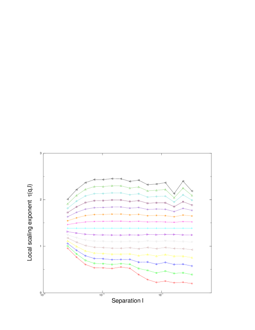
Figure 8: Local scaling exponent obtained as the logarithmic derivative of $M(q,l)$ versus $l$ at time $t=5.8\,\omega_{J}^{-1}$ with Brownian initial velocities. Number of particles is $N=8192$. The exponent $q$ ranges from $0.125$ to $1.875$ in steps of $0.125$.

                        

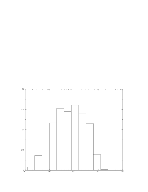
Figure 9: Normalized mass distribution in octaves for Brownian initial velocities at $t=6.0\,\omega_{J}^{-1}$. The number of particles is $8192$, number of independent realizations $30$. Each realization was further averaged over $10^{4}$ collisions, about $2\times 10^{-3}\omega_{J}^{-1}$ in intrinsic time. The height of a column is the fraction of a total number of bins containing mass in the range $[m,2m]$. The bin size is $l=0.003125$, a uniform density would hence correspond to a single column at abscissa $0.003125$ and ordinate $1.0$.

                        

Figure 10: Normalized mass distribution in octaves for BBKS initial velocities at $t=5.9\,\omega_{J}^{-1}$, Number of particles and bin sizes as in fig. 9, number of independent realizations $20$.

                        

Figure 11: Normalized mass distribution in octaves for white noise initial velocities at $t=7.0\,\omega_{J}^{-1}$. Number of particles and bin sizes as in fig. 9, number of independent realizations $10$.

6 Discussion

Observed structures in our universe are believed to have been caused by gravitational instabilities in an initially almost homogeneous medium. The temperature fluctuations of the Cosmic Microwave Background radiation give direct observational access on the primordial density and proper velocity fluctuations which seeded these structures, albeit as of today only on a limited range of scales.

The general problem of structure formation by nonlinear deterministic evolution equations, acting on random initial conditions, is a topic of much current interest, particularly in the context of Burgers’ turbulence, where progress has been made using the special integrability properties of Burgers’ equation. In this paper we have investigated the dynamics of a one-dimensional self-gravitating medium, as a more accurate model of structure formation in the universe. Therefore, it is of interest to understand how different are the solutions to Burgers’ equation and self-gravitating systems starting from the same initial data.

The problem addressed is hence not to determine if these two models are closely similar in general, but if they are similar with specific initial conditions suggested by cosmology. We have focused on Gaussian random fields with scaling spectrum, of the type originally suggested by Harrison and Zeldovich, but with a variable scaling exponent. The main obstacle to a detailed comparison is then to solve numerically the self-gravitating system, since Burgers’ equation is solved directly with the Hopf-Cole transformation. In one spatial dimension we have been able to use an efficient numerical algorithm which exploits a special Lagrangian quasi-invariance of the gravitational force between particle collisions.

A self-consistent formulation of an infinite self-gravitating system demands a background term from the average mass density. This somewhat trivial term changes the properties of the solutions qualitatively compared to those of a finite mass concentration, with zero background. A finite self-gravitating system has a definite center of mass, and particles which are furthest from the center feel the strongest attraction, while in the self-gravitating system with background mass far from the initial perturbation feel no attraction at all. As soon as the system with background has developed structures of much higher density than the background their further development is however quite similar to a finite self-gravitating system: this shows up in the formation of a central body of enhanced density and spiral phase-space structures. A mathematical difference between perturbations in a finite and an infinite self-gravitating system is an effective anti-harmonic term in the latter, which appears when particle density thins out. Since if in the infinite self-gravitating system density can only be less than the average locally if it is higher elsewhere, a thinning out assumes an attractive agglomeration at some other nearby position, which can be seen as the cause of that extra force.

One prediction with analogy with the adhesion model is that for initial perturbations with strong support at low wave numbers, as our case Brownian motion, we expect to see mass agglomerations of very different sizes, while for white noise initial conditions we expect to find most mass agglomerations of similar size. Figs. 9, 11 indeed show this behaviour, while fig. 10 is intermediate.

Summing up, we have shown that one-dimensional self-gravitating dynamics can be investigated quantitatively in systems with a large scaling range in the initial conditions. Nevertheless, the problem remains computationally more demanding than e.g. Burgers’ equation, and our results on the fractal properties of the mass distribution are not conclusive. An improved numerical procedure has been proposed by A. Noullez [22], which would allow us to significantly enhance the resolution and the statistics. Results of this second stage of the investigation will be presented in a forthcoming separate contribution [1].

References

- [1] Aurell E., Fanelli D., Muratore-Ginanneschi P., Noullez A., in preparation
- [2] Aurell E., Frisch U., Noullez A. & Blank M. “Bifractality of the Devil’s staircase appearing in the Burgers equation with Brownian initial velocity”, J Stat Phys. 88, 1151 (1997)
- [3] Bardeen J.M., Bond J.R., Kaiser N. and Szalay A.S., “The statistics of peaks of Gaussian random fields”, The Astrophysical Journal 304 (1986), 15-61.
- [4] Bonvin J.C., Martin Ph.A., Piasecki J. and Zotos X., “Statistics of Mass Aggregation in a Self-Gravitating One-dimensional gas”, (preprint).
- [5] Burgan J.R., Gutierrez J., Munier A., Fijalkow E. and Feix M.R., “Group transformations in phase space fluids” in Strongly Coupled Plasmas, eds. G. Kalman and P. Carini, Plenum press (1978), 597-639.
- [6] Dawson J.M., “One-dimensional plasma model”, The Physics of Fluids 5 (1962), 445-459.
- [7] Eldridge O.C. and Feix M., “One-dimensional plasma model at Thermodynamic equilibrium”, The Physics of Fluids 5 (1962), 1076-1080.
- [8] Feix M., “Computer experiments in one-dimensional plasmas”(appendix by E. Bonomi) in Strongly Coupled Plasmas, eds. G. Kalman and P. Carini, Plenum press (1978), 499-529.
- [9] Gawiser E. & Silk J., “Extracting Primordial Fluctuations”, Science 280 (1998), 1405-1411.
- [10] Gurbatov S.N., Saichev A.I. & S.F. Shandarin S.F.,“The large-scale structure of the Universe in the frame of the model equation of non-linear diffusion”, Monthly Notices of the Royal Astronomical Society 236 (1989) , 385-402.
- [11] Gurbatov S.N., Simdyankin S.I., Aurell E., Frisch U. & Toth G. “On the decay of Burgers turbulence”, J. Fluid Mech. 344 (1997), 339–374.
- [12] Gurevich A.V. & Zybin K.P.,“Large-scale structure of the universe. Analytic theory”, Physics-Uspekhi 38 (1995), 687-722.
- [13] Harrison E.R.,“Fluctuations at the Thresold of Classical Cosmology”, Phys. Rev. D 1 (1970), 2726-2730.
- [14] Jeans J., Proc. Trans. Roy. Soc. 199A (1902), 49.
- [15] Kamionkowsky M., Kosowsky A. “The Cosmic Microwave Background and Particle Physics”, Ann. Rev. Nucl. Part. Sci. (1999), astro-ph/9904108
- [16] Kofman L.A., Pogosyan D., Shandarin S.F. & Melott A.L., “Coherent structures in the universe and the adhesion model”, Astronomical J. 393 (1992), 437-449.
- [17] Kogut A., et al Ap. J. 464 (1996), L29-L33.
- [18] Lifshitz E., J. Phys. USSR 10 (1947), 116.
- [19] Meiksin A., White M., Peackock J.A., Monthly Not. Royal Astr. Soc. 304 (1999), 851.
- [20] Majda A.J., Majda G. & Zheng Y., “Concentrations in the one-dimensional Vlasov-Poisson equation I: Temporal development and non-unique weak solutions in the single component case”, Physica D 74 (1994), 268-300.
- [21] Letters from Sir Isaac Newton to the Reverend Dr. Bentley, Letter I, quoted by S. Weinberg, ref. [34], page 562.
- [22] Noullez A., Private comunication
- [23] Partridge B., 3K: The Cosmic Background Radiation, Cambridge University Press, 1995. Preprint, Princeton University (1997).
- [24] Page L., “Review of Observations of the CMB” Preprint, Princeton University (1997).
- [25] Peebles P.J., The Large-scale Structure of the Universe, Princeton,NJ: Princeton University Press, 1980.
- [26] Roytvarf A. , “On the dynamics of a One-Dimensional Self-Gravitating Medium”, Physica D 73 (1994), 189-204.
- [27] Rouet J.L., M.R. Feix and Navet M., “One-dimensional numerical simulation and homogeneity of the expanding universe”, Vistas in Astronomy 33 (1990), 357-370.
- [28] Rouet J.L. et al, “Fractal properties in the simulation of a one-dimensional spherically expanding universe”, in Lecture Notes in Physics: Applying Fractals in Astronomy (1991), 161-179 .
- [29] Shandarin S.F. and Zeldovich Ya.B., “The large scale structure of the Universe: turbulence, intermittency, structures in a self gravitating medium”, Rev. Mod. Phys. 61 (1989), 185-220.
- [30] She S.-Z., Aurell E. and Frisch U., “The inviscid Burgers equation with initial data of Brownian type” Comm. Math. Phys. 148 (1992), 623-641.
- [31] Sinai Ya.G. “Statistics of shocks in solutions of inviscid Burgers equation” Comm. Math. Phys. 148 (1992), 601-622.
- [32] Smoot G.F. & Scott D., “Cosmic Background Radiation”, Phys. Rev. D 50 (1994), 1173, available as astro-ph/9603157.
- [33] Vergassola M., Dubrulle B., Frisch U. & Noullez A., “Burgers’ equation, Devil’s staircases and the mass distribution for large-scale structures”, Astron. & Astrophys. 289 (1993) 325-356.
- [34] Weinberg S., Gravitation and Cosmology, Wiley (1972).
- [35] Zeldovich Ya.B., Monthly Notices of the Royal Astronomical Society 160 (1972), 1.
- [36] Zeldovich Ya.B. & Novikov I.D., Stroenie i evoljucija vselennoj [The Structure and the evolution of the Universe], Nauka Moscow (1974).